A Fast and Accurate Sparse Continuous Signal Reconstruction by Homotopy DCD with Non-Convex Regularization


Abstract
: In recent years, various applications regarding sparse continuous signal recovery such as source localization, radar imaging, communication channel estimation, etc., have been addressed from the perspective of compressive sensing (CS) theory. However, there are two major defects that need to be tackled when considering any practical utilization. The first issue is off-grid problem caused by the basis mismatch between arbitrary located unknowns and the pre-specified dictionary, which would make conventional CS reconstruction methods degrade considerably. The second important issue is the urgent demand for low-complexity algorithms, especially when faced with the requirement of real-time implementation. In this paper, to deal with these two problems, we have presented three fast and accurate sparse reconstruction algorithms, termed as HR-DCD, Hlog-DCD and Hlp-DCD, which are based on homotopy, dichotomous coordinate descent (DCD) iterations and non-convex regularizations, by combining with the grid refinement technique. Experimental results are provided to demonstrate the effectiveness of the proposed algorithms and related analysis.1. Introduction
Compressive sensing (CS) and sparse signal representation have received widespread attention and increasing interest over the past few years [1,2], which are motivated by the sparse nature of the real world data and the advantages of the CS theory. The applications of CS in numerous areas have been widely investigated in the literature, such as magnetic resonance imaging (MRI) [3], synthetic aperture radar (SAR) imaging [4], inverse synthetic aperture radar (ISAR) imaging [5], passive radar imaging [6], direction-of-arrival (DOA) estimation [7], communication channel estimation [8], seismic signal processing [9], spectral estimation [10], image processing [11], speech enhancement [12], etc. Generally speaking, those disciplines explore the following linear signal model [13]:
1.1. Off-Grid Problem in CS-Based Methods
In the CS processing procedure, the first necessary step is to design a dictionary through a discretization operation with the assumption that the elements of unknown x lie exactly on those pre-defined grids corresponding to A. Obviously, this is practically impossible since the continuous nature of the unknowns of x, such as the unknown directions, may not fall into the predefined angular grids in DOA, and the scatterers of the target may not locate exactly on the pre-discretized scene grids in radar imaging. Hence, once faced with a continuous signal, the off-grid problem in using the conventional sparse recovery techniques is inevitable, no matter how densely we grid x. Previous researches [15–17] have demonstrated that the traditional CS-based methods would be severely affected when the off-grid problem emerges, and [18] also claimed that the off-grid problem is one of the major constraints in popularizing CS-based methods in practice. It is worth noting that there may be other factors leading to basis mismatch, for example, in the radar imaging field, unsatisfactory system parameters (e.g., position errors of transceivers [19] and phase synchronization mismatch [20]) are also likely to degrade the performance of conventional CS-based methods from our previous researches, however this paper only focuses on the off-grid problem, and assumes the system errors are small enough.
The solutions for off-grid problem have been broadly studied in previous literatures [21–30]. So far, main research topics include three types as follows:
- (a)
Direct method according to theories of Xampling and the finite rate of innovation (FRI). This scheme is first introduced by Michaeli et al. as a general framework within various solutions for analog signals [21]. The significant advantage of this method is its direct solution, without any pre-discretization of the continuous signal at first. Thus it is less sensitive to off-grid problem compared with traditional CS-based methods. However, this method is mainly based on spectral estimation algorithms (e.g., ESPIRT [22], MUSIC [6], Matrix Pencil [23]), which needs special signal expression in linear measurement model and its performance may suffer from low SNR and few snapshots [24].
- (b)
Off-grid CS method. This kind of method is under a first order Taylor expansion model, and thus is quite sensitively depended on the model's accuracy, and cannot give a thorough solution when higher order approximations are significant [23]. Furthermore, it is likely to involve highly-computational burden [25,26] for alternatively finding the sparse solution and estimating the off-grid error, especially in large scale problem.
- (c)
Grid refinement approach. The idea of the grid refinement technique was firstly introduced by Malioutov et al. [27] to mitigate the effect of limiting estimates to a grid of spatial locations in source localization problem. Then it is generalized by Liu et al. [28] for locating two-dimensional multiple underwater acoustic sources. Recently, Guldogan et al. [29] have proposed a novel grid refinement algorithm to alleviate off-grid problem by using a particle swarm optimization (PSO) and orthogonal matching pursuit (OMP), which makes use of the PSO to perturb the location of each grid point.
Since the “grid refinement approach” is iteratively refined to match with the desired resolution of the off-grid components by “coarse and fine grid partition” operations, and does not have the drawbacks of (a) and (b), this paper follows the idea of “grid refinement approach” which makes a coarse grid first instead of having an universally fine grid to reduce the complexity, then achieves fine grids around the peaks using more refinement levels. In this way, after a few iterations of refining process, it becomes fine enough that off-grid problem effect is negligible.
1.2. Fast and Efficient Algorithms for Real-Time Implementation
Furthermore, there exists another common challenge by utilizing the CS-based methods, i.e., we need fast and efficient algorithms for real-time system implementation, particularly for digital electronic circuits (e.g., ARM, FPGA, DSP) [30]. From previous researches, sparse recovery techniques can be roughly divided into two families, that are greedy methods (e.g., MP [31], OMP [32], GP [33]) and optimization based methods (e.g., l1 optimization [34], smoothed l0 optimization [35], non-convex optimization [36]). Generally speaking, greedy methods have the advantages of lower complexity, faster speed, less storage requirement, and flexible implementation compared with optimization based methods, and are considered the most suitable candidates for hardware implementation. However, their performances are inferior to those of the optimization based methods, such as l1 norm minimization basis pursuit de-noising (BPDN) [34].
As the coordinate descent (CD) search has an inherent property of being low complexity when signals are sparse, Zakharov et al. have successfully exploited dichotomous CD (DCD) iterations for solving LS [37], RLS [38] and MVDR beamforming problems [39] using FPGAs for real-time implementation. In addition, to solve the reweighted l1 minimization problem, they have developed a greedy algorithm called Hl1-DCD [40], i.e., homotopy DCD method with reweighted l1 penalty, which has shown a high recovery performance with relatively low complexity. It turns out that the overall complexity of the algorithm is comparable to that of MP. Moreover, homotopy iterations result in high accuracy of the solution, even higher than that of the YALLl algorithm. Meanwhile, Liu and Zakharov et al. [28] have utilized the low complexity homotopy approach combined with CD search for locating underwater acoustic sources by solving the multi-frequency BPDN problem. The proposed method is evaluated by applying to simulated and real experimental data. As far as we know, previous studies [28,37–40] are mainly focusing on homotopy DCD with convex regularizations, while there are seldom researches linking to homotopy DCD with non-convex regularizations.
1.3. Our Contribution
From the above discussion, we have addressed two major issues (i.e., off-grid problem and efficient algorithms for real-time implementation) of applying CS to sparse continuous signal reconstruction. In this paper, motivated by the idea of Hl1-DCD [40] and grid refinement approach [27], we present three fast and accurate sparse reconstruction algorithms (i.e., HR-DCD, Hlog-DCD and Hlp-DCD) which are based on homotopy, dichotomous coordinate descent (DCD) iterations and non-convex regularization, combining with the grid refinement technique to deal with the aforementioned issues. The main contributions of this paper are as follows: (1) we formulate the sparse recovery problem by homotopy DCD method with three typical classes of non-convex penalties, which are proved to recover sparsity in a more efficient way than homotopy DCD method with convex penalties as shown in Zakharov's previous researches [28,37–40]; (2) further, the grid refinement technique [27] is utilized to combine with our algorithms to alleviate the effect of off-grid problem and reduce the complexity simultaneously; (3) experimental results of three representative applications (DOA, passive radar imaging, ISAR imaging) are carried out to verify the effectiveness of the proposed methods.
The outline of this paper is as follows: in Section 2, two sparse recovery problems are discussed. Section 3 describes the proposed methods and related analysis. In Section 4, extensive experimental results are presented to verify our methods. Finally, Section 5 draws the conclusions.
Throughout this paper we shall make use of the following notation: bold-case letters are reserved for vectors and matrices, e.g., x is a vector, A is a matrix; Elements of A and x are represented as An,p and xn, respectively. I and Ic denote the support and its complement, respectively. Further, we represent by R(q) the q-th column of R; AI a matrix obtained from A keeping only columns corresponding to I; xI the subset of x that contains entries from x corresponding to I; ‖x‖p denotes the lp norm of a vector, ‖A‖2 is the spectral norm of the matrix A; 〈,〉 denotes the inner product; (·)H, (·)*, Re{·}denote the conjugate transpose, conjugate and real part operations, respectively.
2. Problem Formulation and Motivations
This section briefly introduces the general sparse recovery framework, upon which we develop our algorithms. As stated before, various applications can be represented by the linear model as Equation (2) shows.
When considering the practical applications, sparse recovery techniques require low-complexity algorithms just as some kinds of greedy methods which are suitable for real-time implementation. However, the performances of greedy methods are compared unfavorably with optimization based methods (e.g., using l1 norm, reweighted l1 norm, lp norm, smoothed l0 regularization). Recently, Zakharov et al. have proposed the homotopy DCD method with convex regularizations, including l1 and reweighted l1 norms, which have shown a high recovery performance and relatively low complexity. Moreover, most of the operations in the algorithms are additions, therefore, they are very suited for the hardware implementation of real-time operating systems. Motivated by the idea of homotopy DCD method and the fact that non-convex regularization usually yields a sparser solution than any convex penalty for a given residual energy (see Figure 1 for example), this paper proposes a fast and accurate sparse signal reconstruction by homotopy DCD technique with non-convex regularizations. Three typical non-convex penalty functions [12,41] are considered, i.e., the first order rational function penalty, the logarithmic penalty and the lp penalty, respectively. With the corresponding penalties, we have achieved the derivation of the HR-DCD, Hlog-DCD and Hlp-DCD algorithms in the next section.
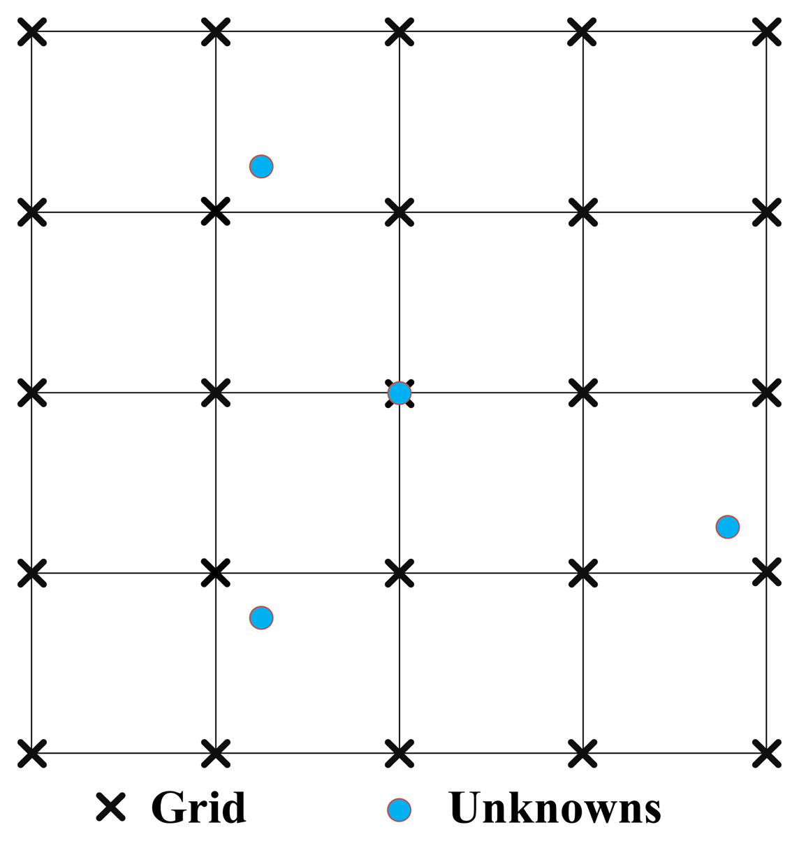
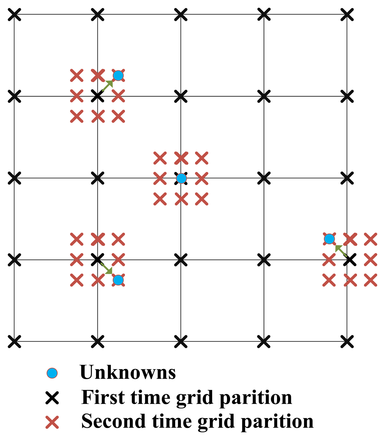
Since x is usually distributed continuously in the corresponding space in many applications, the off-grid problem is likely to exist. For example, in the radar imaging field, the reflectivity centers of the scatterers are generally not located at exact on-grid spatial positions illustrated in Figure 2, which means the measurement matrix should cover the basis vectors corresponding to off-grid scatterers. As conventional CS-based methods do not consider the off-grid effect, therefore the related sparse reconstruction techniques suffer unacceptable degradation in image quality. This paper has utilized the grid refinement approach [27] shown in Figure 3 combined with the HR-DCD, Hlog-DCD and Hlp-DCD algorithms to alleviate the impact of off-grid problem (see details in Section 3.2). Experimental results in Section 4 are provided to demonstrate the performance improvement of the proposed algorithms.
3. Homotopy DCD with Non-Convex Regularization Algorithms
We consider minimization of the following cost function to solve the problem Equation (2):
- (a)
The first order rational function penalty:
- (b)
The logarithmic penalty:
- (c)
The lp penalty:
In order to reduce the complexity of the DCD algorithm, we develop a greedy algorithm that is based on homotopy method with respect to a set of the parameter τ. Besides, the updates of our DCD algorithm are only done within the support instead of all elements. As the support is usually much smaller than N, therefore, the complexity is further reduced. We consider the first order rational function penalty at first, and develop HR-DCD algorithm. Then Hlog-DCD algorithm and Hlp-DCD algorithm can be similarly obtained.
The following two propositions define the rules for adding/removing elements into/from the support of HR-DCD algorithm.
Let I be the support at some homotopy iteration, and Ic be its complementary set. Denote r = y − Ax, R = AH A and b = AH r.
Proposition 1: Add the t-th (t ∈ Ic) element into the support I according to the rule:
We now prove Proposition 1.
Proof: Let the t-th element xt = 0 be activated as x̂ = α = |α|e jarg{α}, and the updated solution vector is denoted as x̂ The update of the cost function Equation (3) is then given by:
The cost function is reduced if ΔJ < 0. For a fixed |α|, ΔJ achieves a minimum value if arg{α} = arg{bt}, and in this case:
Let:
For |α| > 0, if , we have:
If ΔJ′ < 0, then 4aRt,t τ − (Rt,t + a|bt|)2 < 0. Thus, there exists a value of α that results in ΔJ < 0, i.e., in reducing the cost function. It is seen from the last expression that if we want to add a new element to the solution vector, the index t of the element should correspond to the maximum of over t ∈ Ic. In this case, we will obtain the largest decrement of the cost function.
Thus, the value of α that for a fixed t such that 4aRt,t τ − (Rt,t + a|bt|)2 < 0 results in the decrement of the cost function is given by:
According to the above statements, the (n + 1)-th nonzero element to be activated in x̂ should satisfy:
For |α| > 0, we have:
If (Rt,t + a|bt|)2 < 4aRt,t τ, then in this case:
Therefore, if |α|> 0 then for (Rt,t + a|bt|)2 < 4aRt,t τ, we have ΔJ > 0, i.e., the cost function increases.
We now prove the Proposition 2:
Proof: Let the t-th element xt ≠ 0 be activated as x̂t = 0 and the updated solution vector is denoted as x̂. The update of the cost function is then given by:
Combining the DCD algorithm in Table 1 and the above two propositions, we arrive at the HR-DCD algorithm presented in Table 2.
The HR-DCD algorithm starts with the zero support I = Ø, and τ = |bt|. For each τ, it updates the support and minimizes the cost function according to the corresponding propositions. Besides, the algorithm will terminate if the iteration times reach the preset parameter L or τ ≤ τmin (τmin is a predefined parameter).
Remark 1: When the penalty is logarithmic function, we give two similar propositions as follows:
Proposition 3: Add the t-th (t ∈ Ic) element into the support according to the rule:
Proposition 5: Add the t-th (t ∈ Ic) element into the support according to the rule:
The proofs for Equations (18)–(21) will be shown in the Appendix. By combining the corresponding propositions with related DCD algorithms, it is easy to obtain Hlog-DCD algorithm and Hlp-DCD algorithm, respectively, and we omit the tabulated expressions here for simplicity.
3.1. Complexity Analysis
The complexity is given by P ≅ 8MN + 4NL + 2CuN +Ci +2NdebLg The term 8MN is for computing the initial b. The term 4NL is for selection of elements in the support. The term 2CuN is for updating b in the total number Cu of successful DCD iterations, and each update requires only 2N real valued additions, as multiplications by αt are bit-shifts. The term Ci takes into account Ci (total number of DCD iterations) tests to decide if the DCD iteration is successful. The debiasing (2NdebLg) is now done by using extra Ndeb DCD iterations on the finally identified support with size Lg.
3.2. Off-Grid Problem Solution
As stated before, we explore the idea of grid refinement technique [27] to reduce the number of the arbitrarily located potential positions of x. Two-dimensional passive radar imaging is selected as an example to illustrate the procedures of solution, which is realized as follows:
- (1)
Under a coarse resolution Δxq, Δyq, where Δxq, Δyq represent the range step and azimuth step respectively, calculate the coarse localizations (xn, yn), = 1, ⋯, S results by finding S largest amplitude peaks using the proposed algorithms, i.e., HR-DCD, Hlog-DCD and Hlp-DCD.
- (2)
Build a denser grid around the estimated locations (xn, yn) with a finer resolution (Δxq, Δyq) as Figure 2 mentioned in Section 2.
- (3)
Set q = q + 1 and , , repeat for Q times from Step (1) until the desired resolution is achieved.
In order to reduce the multiplications, we use dichotomy for grid refinement, which can use bit-shifts instead of multiplications to be implement in hardware system. According to our experimental results in Section 4, no more than 10-step grid refinement process is needed.
3.3. Extension to Multiple Measurement Vectors (MMV) Case
Although we have derived HR-DCD, Hlog-DCD and Hlp-DCD algorithms from a single measurement vector (SMV), the results can be generalized to MMV case. In some kinds of applications, such as wideband source localization [42], multiple frequency bins are explored. As we all know that single frequency results can be easily disturbed by noise and interference, and in this issue, we can use a frequency diversity to achieve better performance. A traditional method of modifying the above approach to multi-frequency signals is averaging the results of all the frequencies. But due to the presence of noise, environmental mismatch and interference, different frequencies may give different results, thus this combining method may not work well.
By the similar approach used in [28], our proposed methods require that for all frequencies to have the same support, which utilize the joint sparsity pattern, and choose an element to add to the support according to the corresponding propositions to achieve greater frequency diversity and avoid the possible wrong results. And the final result can be given by averaging all the results of all the frequencies through this way.
4. Experimental Results
In this section, we will present several simulation results which illustrate the effectiveness of the proposed methods. All experiments are performed by using MATLAB R2013a on a PC equipped with an Inter Core i7 3770k CPU, 3.5GHz and 32 GB memory. The state-of-the-art sparse recovery methods such as MP, BP, FOCUSS, SBL, Hl1-DCD, etc. are selected for comparison. As a benchmark we will utilize an oracle sparse recovery (OSR) to represent the best inversion performance, which knows the true support of x. In addition, we set parameter a = 10 in Equation (4) for HR-DCD, in Equation (5) for Hlog-DCD, and p = 0.8 in Equation (6) for Hlp-DCD, and Mb = 10, τmin = 0.02, γ = 0.9 by experience from extensive simulation results. Other predefined parameters such as H, L, S, and the grid refinement times Q, etc., are decided according to the actual conditions, which will be given in details in the next text.
4.1. DOA Estimation
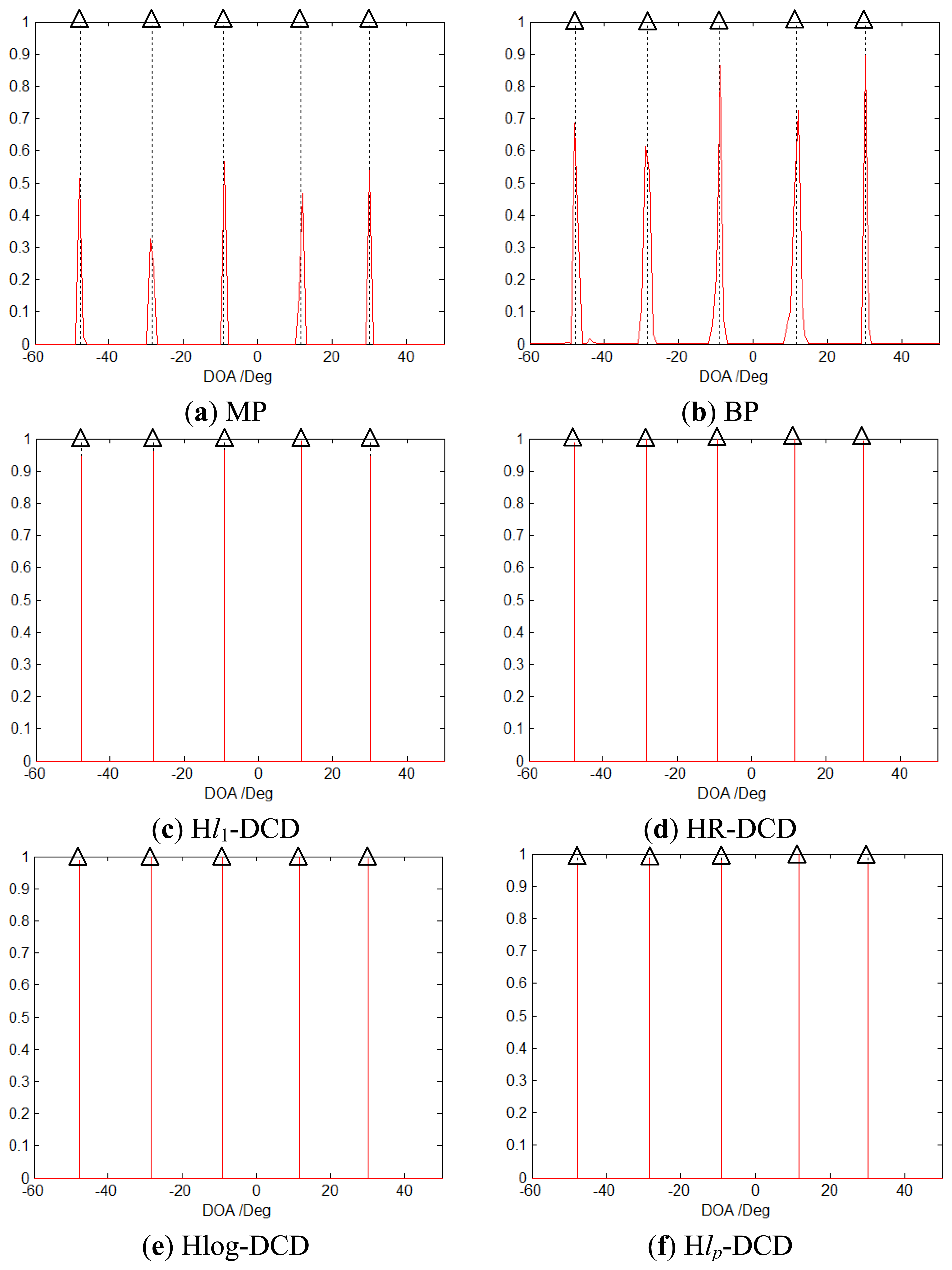
As described by Malioutov et al., for one snapshot case, the DOA problem of Equation (5) in [27] is equivalent to Equation (2) in this paper. With the assumption that the sources can be viewed as point sources and their number is small, the underling spatial spectrum is sparse and it can be solved via sparse recovery methods mentioned above. The first simulation considers the scenario that there are five uncorrelated signals impinging from [−47.7°, −28.5°, −9.2°, 11.6°, 30.1°]. The grid is set to be within the range of −90° to 90° with 1° spacing. A 30-element uniform linear array (ULA) spaced in half-wavelength units is used, and the signal-to-noise ratio (SNR) is set to be 20 dB. Here we only consider one snapshot case, and set H = 1, L = S = 8, Q = 10. Figure 4 depicts the solutions solved by different methods, and the vertical dashed lines mark the true directions. Obviously, our methods find the positions and the amplitudes exactly and achieve much sparser solutions than MP and BP. Moreover, they have a better amplitude estimation than Hl1-DCD [40].
We give a time cost for the aforementioned methods in Table 3. From the results, we can see that our methods have the same time cost as the Hl1-DCD. Although they are a little longer than MP, but they are much less costly than BP. However, the significant advantages of our methods are that they are very easy to implement in a hardware platform because only bit-shifts are needed instead of multiplications similar as [37–40], besides, they can achieve the similar reconstruction performance as BP without off-grid problem.
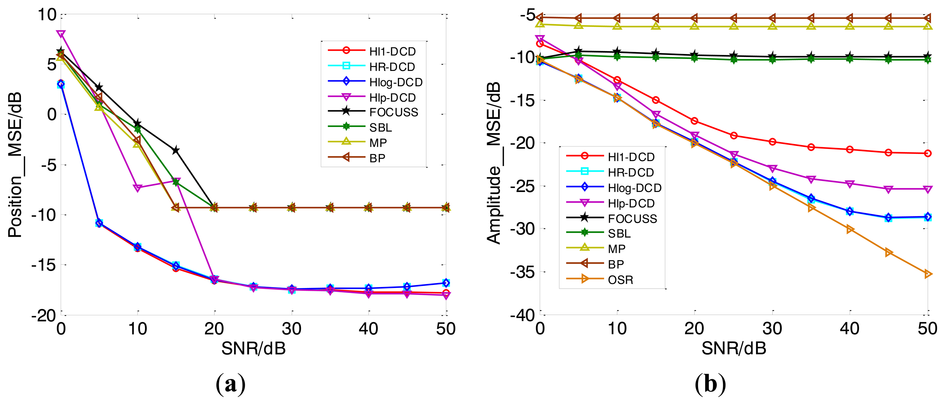
Next we compare the mean squared error (MSE) of position and amplitude estimation performances by applying the proposed methods and several popular methods (MP, BP, FOCUSS, SBL, Hl1-DCD, OSR), which are defined as follows:
Figure 5a compares the MSEs of DOA estimation results of different methods under varying SNR, which are averaged by 100 Monte Carlo trials. From the curves of MSE of position versus SNR shown in Figure 5a, it can be seen that Hl1-DCD and the proposed methods have similar results in position estimation, and outperform their counterparts. However, our methods have better amplitude estimation accuracy than Hl1-DCD from Figure 5b, and are even very close to the OSR performance.
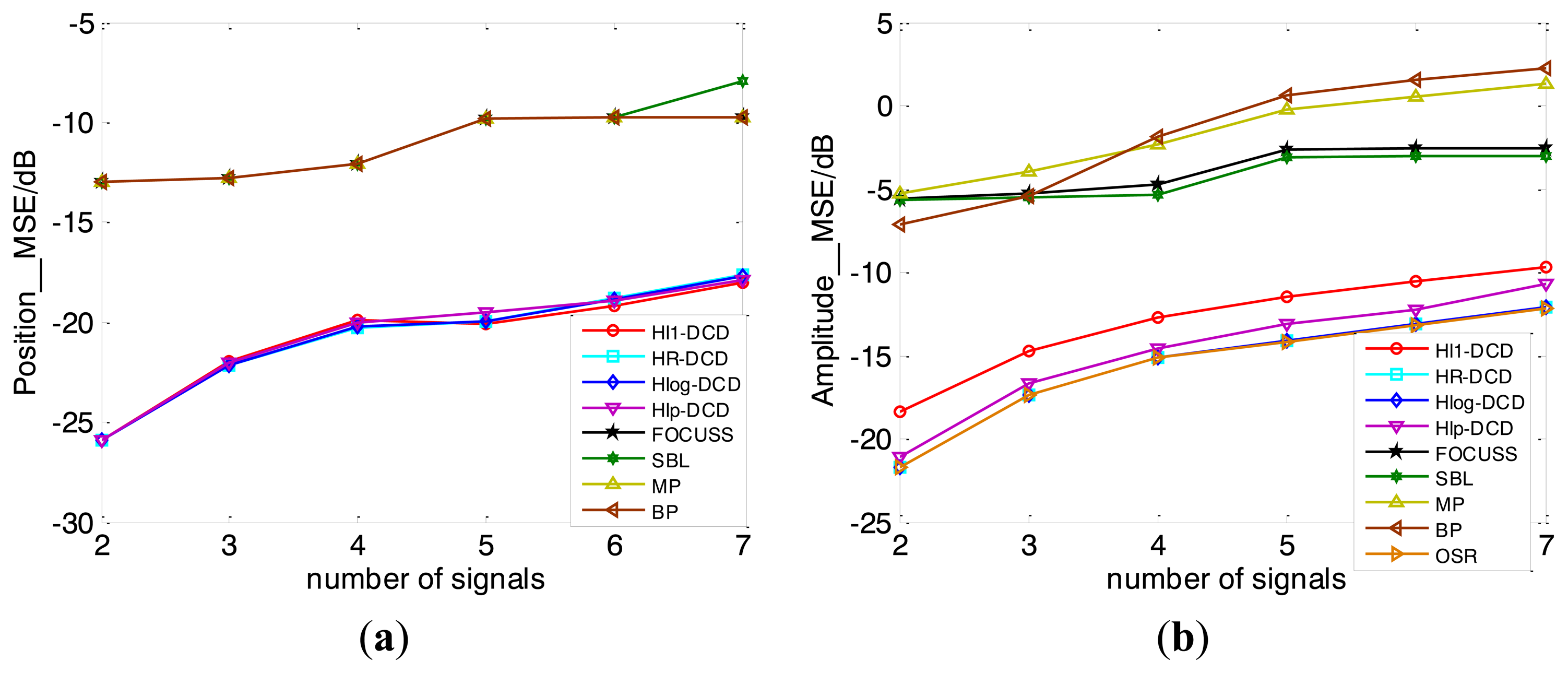
The MSEs of DOA estimation versus number of signals shown in Figure 6 are obtained over 100 Monte Carlo trials with SNR equals to 20 dB. We can clearly see that our methods perform best compared to other methods with the same parameters, especially on the amplitude estimation results.
4.2. Passive Radar Imaging
In this part, we aim to test the performance of the proposed methods in a passive radar imaging system. Based on the final echo Equation (17) stated in [6] which is similar to Equation (2) in this paper, sparse recovery techniques can be utilized to solve the problem of passive radar imaging. In the simulation, we choose seven digital video broadcasting (DVB) satellites as opportunity transmitters and 10 receivers, and the initialization grids are 21 × 41 represented for the imaging scene 20 m × 20 m (here we use the axis function in matlab to make the scene limited to be 12 m × 10 m so as to achieve a better visual effect). There are nine off-grid scatterers with different reflection coefficients in the scene of interest as the red circles illustrated in Figure 7. The number of frequency samplings corresponding to each transmitter is 10, and the SNR equals to 20 dB. Other simulation parameters are the same as displayed in [6]. Here we set H = 2, L = S = 10 and grid refinement times Q = 10.
Figure 7a shows the poor imaging result by BP due to the reason that in practice the scatterers are not located exactly on the pre-discretized grids, and the echoes are mismatched with the measurement matrix, therefore the performances of CS-based reconstructions are generally unsatisfactory. Figure 7b is the imaging result by Hl1-DCD, and we can see that it can seek the exact locations of the target, however the amplitude estimation of the reflection coefficients is not precise.
Figure 7c–e represents the imaging results by the proposed methods. As expected, the proposed methods do not have the off-grid problem from the perspective of both the position and amplitude estimation results, which show the potential of our methods to be applied in practical passive radar system.
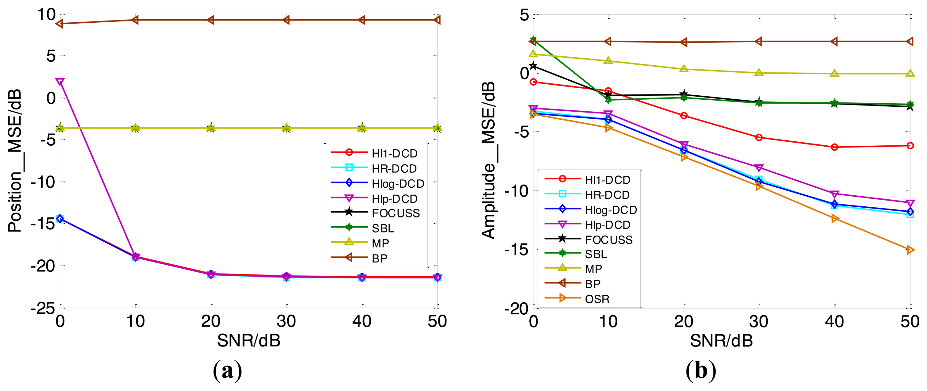
Figure 8 shows the MSEs of position and amplitude estimation results versus SNR by applying different methods, which are averaged over 100 Monte Carlo trials. In the simulation, we have assumed that there are nine off-grid scatterers with unit reflection coefficients distributed randomly in imaging region. It is seen that our methods outperform the conventional methods (MP, BP, FOCUSS, SBL) in further improvement of MSEs of position and amplitude estimates when off-grid target emerges. In the meantime, they have better amplitude estimation result than Hl1-DCD with the same parameters shown in Figure 8b. Moreover, the performances of our methods approach the OSR very closely under varying SNR, both in position and amplitude estimates.
4.3. ISAR Imaging
We utilize the CS ISAR imaging model as discussed in [43], and assume that the translational motion compensation has been already achieved and thus only the rotational motion is considered. The relation between the received signal and the complex reflection coefficients can be written as Equation (10) in [43], which is equivalent to Equation (2) in this paper.
We use the quasi real data of an airplane (B-727) provided by the U.S. Naval Research Laboratory to test the feasibility and performance of the proposed methods, which is available on the website http://airborne.nrl.navy.mil/∼vchen/tftsa.html. The stepped frequency radar operates at 9 GHz with the equivalent pulse repetition interval (PRI) of 3.2 ms and has a bandwidth of 150 MHz. For each pulse train, 64 complex range samples were saved, and the file contains 200 successive pulse trains within the long coherent processing interval (CPI). An additive noise is added to the original B-727s data, and the SNR is set to 10 dB. Herein we choose 40 range cell numbers and 20 cross range cell numbers for short CPI test, and the reconstruction of target spatial domain is discretized with 64 range bins and 32 cross range bins, besides, we set H = 2, L = S = 60 and Q = 5. Since in radar imaging field, the position estimates are very important when off-grid problem exists.
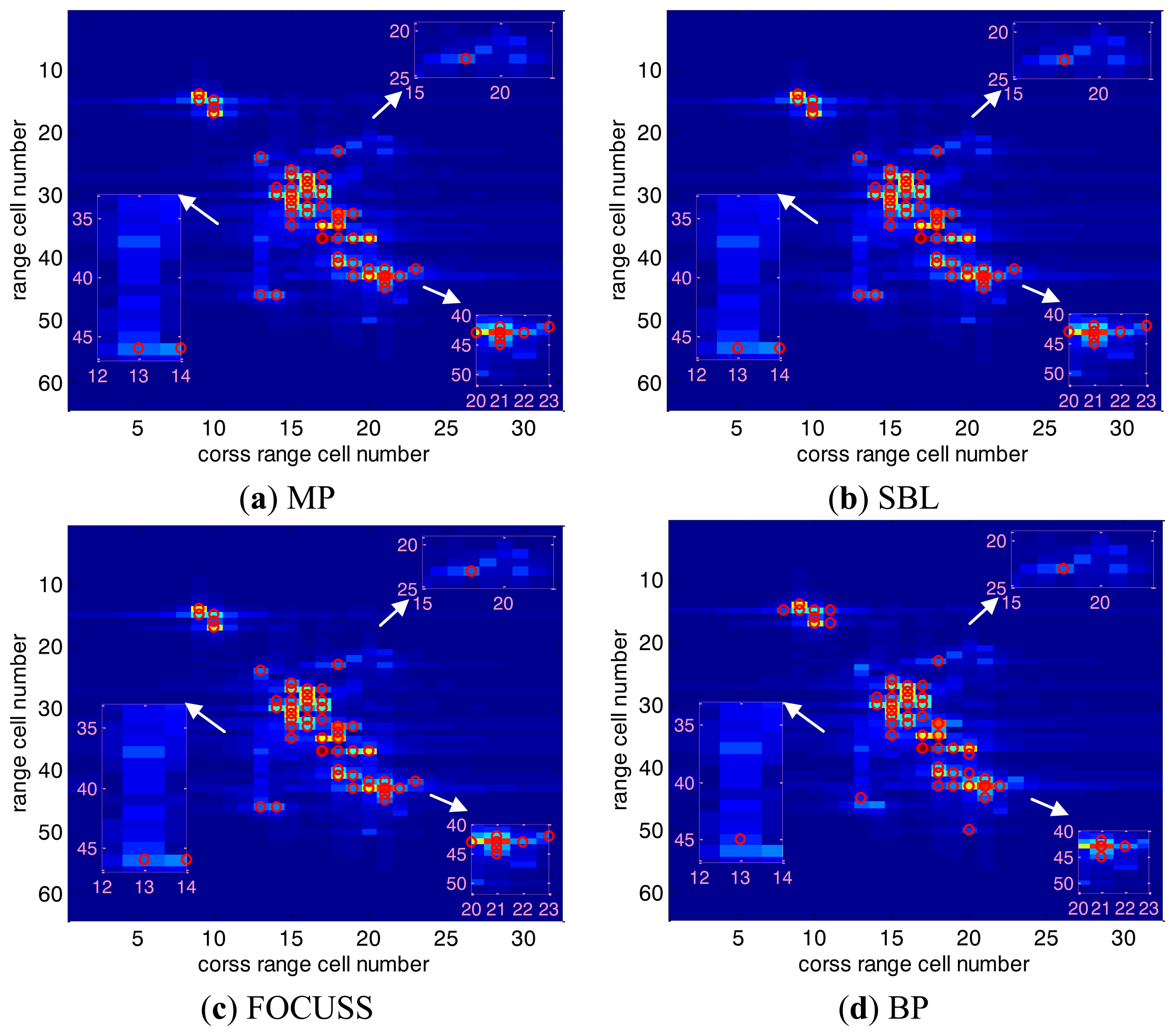
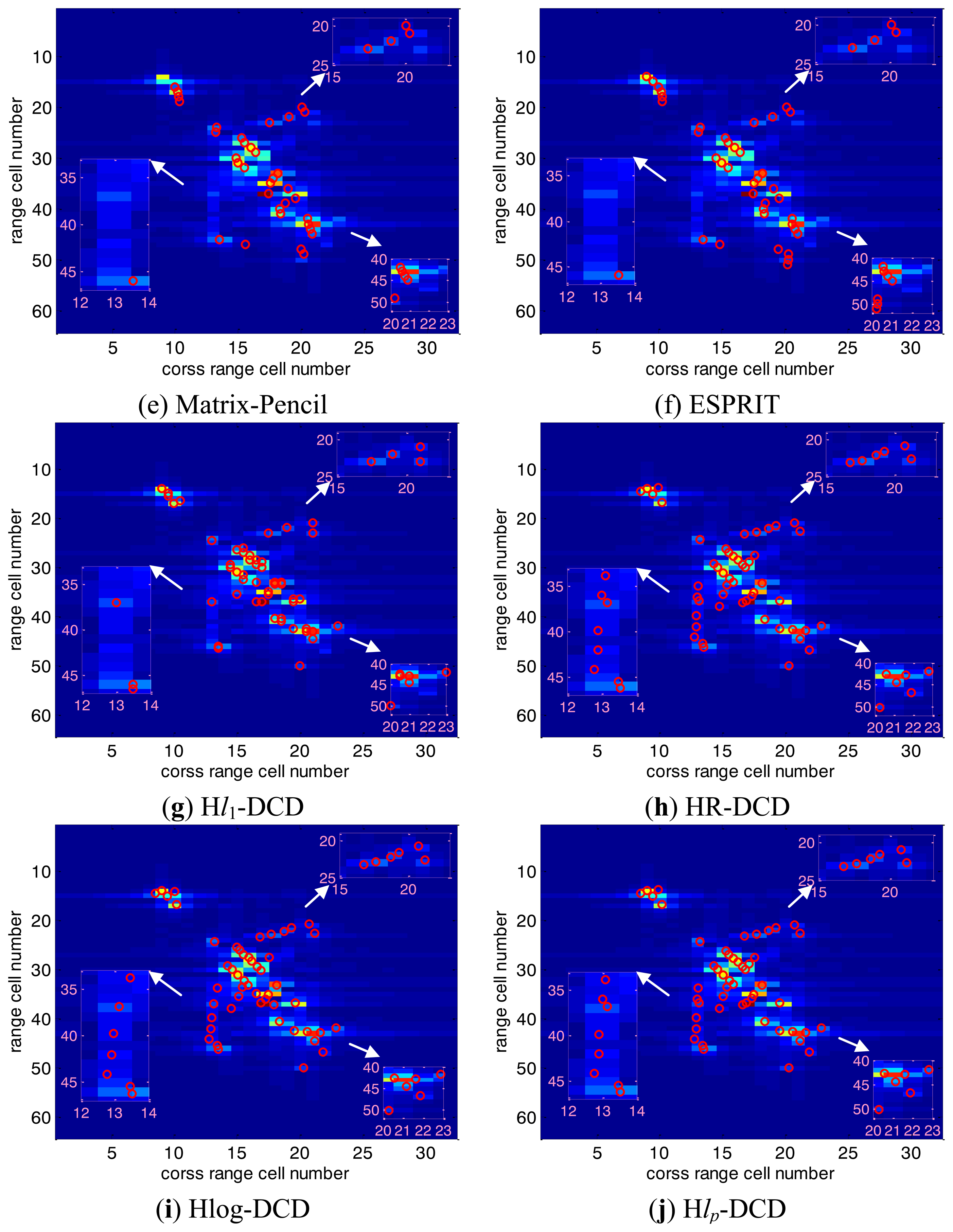
Figure 9 are the position recovery results by MP, SBL, FOCUSS, BP, Matrix-Pencil, ESPRIT, Hl1-DCD and the proposed methods (HR-DCD, Hlog-DCD and Hlp-DCD) shown as the red circles, and we use the conventional FFT-based ISAR image as the background for fair comparison. As stated above, the imaging performances of the classical methods (MP, BP, FOCUSS, SBL) are not good because of the off-grid errors. Matrix Pencil and ESPRIT can direct solve the positions of the plane, but their performances suffer from low SNR and few snapshots, therefore the imaging results are not good enough. In contrast, our methods can deal with the off-grid target, and achieve satisfying imaging performances which have better visual effect for the airplane shape. Moreover, it is obvious that the imaging results of our methods are better than Hl1-DCD with the same parameters, especially on the details of airplane wings and tails as illustrated in zoomed-in regions of Figure 9h–j, which demonstrate the advantage of homotopy DCD method with non-convex regularization compared with convex regularization under the same measurements.
In order to quantitatively evaluate the amplitude estimation performances of the obtained ISAR images via different methods, we use the correlation value [44] to evaluate the similarity between the recovered images and the reference image, and the image entropy [44] to measure the focusing quality of the recovered images. They are defined as follows:
The correlation and entropy values of the recovered ISAR images under different methods are summarized in Table 4. It can be seen that the proposed methods have a higher correction with the reference image and a lower entropy than their counterparts, and thereby exhibit a better capability of target-information extraction.
5. Conclusions
Two major problems of applying CS to sparse continuous signal reconstruction are discussed in this paper, and we have presented computationally efficient and accurate methods to overcome the difficulties. For solving the off-grid problem, we utilized the grid refinement technique. In the meantime, in order to obtain high recovery performance and keep low calculation complexity, we propose a fast and accurate homotopy DCD reconstruction combined with three typical non-convex regularizations, which promotes sparsity more strongly than any convex penalty function can. Extensive experiments have been conducted to validate and compare the performances of the proposed methods with several popular solvers. Our future work will try to synthesize with parallel sparse optimization technique using multi-core CPUs/GPUs [45], which may provide a viable solution to real-time potential applications.
Acknowledgments
The work is supported by the General Program of National Natural Science Foundation of China under Grant No. 61172155, and the Hi-Tech Research and Development Program of China under Grant No. 2013AA122903. Moreover, the authors would like to thank Li Ding and ChangChang Liu for support and fruitful discussions.
Author Contributions
All authors contributed extensively to the work presented in this paper. Tianyun Wang designed the study, analyzed the data and wrote the paper; Xinfei Lu, Tianyun Wang and Xiaofei Yu designed and performed the experiments; Weidong Chen and Zhendong Xi supervised its analysis and edited the manuscript, and provided their valuable suggestions to improve this study.
Conflicts of Interest
The authors declare no conflict of interest.
Appendix
Remark 1: the Penalty is Logarithmic Function.
Proof for Proposition 3: Let the t-th element xt = 0 be activated as x̂t = α = |α|e jarg{α}, and the updated solution vector is denoted as x̂. The update of the cost function is then given by
The cost function is reduced if ΔJ < 0. For a fixed |α|, ΔJ achieves a minimum if arg{α} = arg{bt}, and in this case
As we can see, if |α| = 0, then ΔJ = 0. So if , when|α| > 0, there exists a |α| that makes ΔJ < 0.
If , we can get
Therefore, if |bt| > τ, there exists a |α| that decreases the cost function.
Proof for Proposition 4: Let the t-th element xt ≠ 0 be activated as x̂t = 0, and the updated solution vector is denoted as x̂. The update of the cost function is then given by
Thus, if , then ΔJ < 0, there exists a nonzero value of the t-th element that decreases the cost function that should be removed from the support.
Remark 2: The Penalty is lp Norm Function.
Proof for Proposition 5: Let the t-th element xt = 0 be activated as x̂t = α = |α|e jarg{α}, and the updated solution vector is denoted as x̂. The update of the cost function is then given by
The cost function is reduced if ΔJ < 0. For a fixed |α|, ΔJ achieves a minimum if arg{α} = arg {bt}, and in this case
From Equation (30) we can see that if and , then ΔJ < 0.
Thus, the value of |α| results in the decrement of the cost function is given by
And we can get the proposition that if , the t-th element would be added into the support.
Proof for Proposition 6: Let the t-th element xt ≠ 0 be activated as x̂t = 0, and the updated solution vector is denoted as x̂. The update of the cost function is then given by
Thus, if , then ΔJ < 0, there exists a nonzero value of the t-th element that decreases the cost function that should be removed from the support.
References
- Donoho, D.L. Compressed sensing. IEEE Trans. Inform. Theory 2006, 52, 1289–1306. [Google Scholar]
- Candes, E.J.; Wakin, M.B. An introduction to compressive sampling. IEEE Signal Process. Mag. 2008, 25, 21–30. [Google Scholar]
- Lustig, M.; Donoho, D.; Pauly, J.M. Sparse MRI: The application of compressed sensing for rapid MR imaging. Mag. Reson. Med. 2007, 58, 1182–1195. [Google Scholar]
- Wei, S.J.; Zhang, X.L.; Shi, J.; Xiang, G. Sparse reconstruction for SAR imaging based on compressed sensing. Prog. Electromagn. Res. 2010, 109, 63–81. [Google Scholar]
- Zhang, L.; Xing, M.D.; Qiu, W.C.; Li, J.; Sheng, J.L.; Li, Y.C.; Bao, Z. Resolution enhancement for inversed synthetic aperture radar imaging under low SNR via improved compressive sensing. IEEE Trans. Signal Process 2010, 48, 3824–3838. [Google Scholar]
- Wang, T.Y.; Liu, C.C.; Lu, H.C.; Chen, W.D. Sparse Passive Radar Imaging Based on Digital Video Broadcasting Satellites Using the Music Algorithm. Proceedings of International Conference on Signal Processing (ICSP), Beijing, China, 21–25 October 2012; pp. 1925–1930.
- Hyder, M.M.; Mahata, K. Direction-of-arrival estimation using a mixed l2,0 norm approximation. IEEE Trans. Signal Process 2010, 58, 4646–4655. [Google Scholar]
- Meng, J.; Yin, W.T.; Li, Y.Y.; Nguyen, N.T.; Han, Z. Compressive sensing based high resolution channel estimation for OFDM system. IEEE J. Sel. Top. Signal Process 2012, 6, 15–25. [Google Scholar]
- Wang, Y.F.; Cao, J.J.; Yang, C.C. Recovery of seismic wavefields based on compressive sensing by an l1-norm constrained trust region method and the piecewise random subsampling. Geophys. J. Int. 2011, 187, 199–213. [Google Scholar]
- Polo, Y.L.; Wang, Y.; Pandharipande, A.; Leus, G. Compressive Wide-band Spectrum Sensing. Proceedings of IEEE International Conference on Acoustics, Speech and Signal Processing (ICASSP), Taipei, Taiwan, 19–24 April 2009; pp. 2337–2340.
- Yang, A.; Zhou, Z.H.; Balasubramanian, A.; Sastry, S.; Ma, Y. Fast l1-minimization algorithms for robust face recognition. IEEE Trans. Image Process 2013, 22, 3234–3246. [Google Scholar]
- Chen, P.Y.; Selesnick, I.W. Group-Sparse Signal Denoising: Concave Regularization, Convex Optimization. Available online: http://arxiv.org/abs/1308.5038 (accessed on 30 November 2013).
- Eldar, Y.C.; Kutyniok, G. Compressed Sensing: Theory and Applications; Cambridge University Press: Cambridge, UK, 2012. [Google Scholar]
- Candès, E.J. Compressive sampling. Proceedings of the International Congress of Mathematicians (ICM), Madrid, Spain, 22–30 August 2006; pp. 1433–1452.
- Chi, Y.J.; Scharf, L.L.; Pezeshki, A.; Calderbank, A.R. Sensitivity to basis mismatch in compressed sensing. IEEE Trans. Signal Process 2011, 59, 2182–2195. [Google Scholar]
- Ugur, S.; Arikan, O.; Gurbuz, A.C. Off-grid Sparse SAR Image Reconstruction by EMMP Algorithm. Proceedings of IEEE Radar Conference, Ottawa, Canada, 29 April–3 May 2013; pp. 1–4.
- He, X.Z.; Liu, C.C.; Liu, B.; Wang, D.J. Sparse frequency diverse MIMO radar imaging for off-grid target based on adaptive iterative MAP. Remote Sens. 2013, 5, 631–647. [Google Scholar]
- Gurbuz, A.C.; Teke, O.; Arikan, O. Sparse ground-penetrating radar imaging method for off-the-grid target problem. J. Electron. Imaging 2013, 22. [Google Scholar] [CrossRef]
- Liu, C.C.; Chen, W.D. Sparse selfcalibration imaging via iterative map in FM-based distributed passive radar. IEEE Geosci. Remote Sens. Lett. 2013, 10, 538–542. [Google Scholar]
- Ding, L.; Liu, C.C.; Wang, T.Y.; Chen, W.D. Sparse Self-calibration via Iterative Minimization Against Phase Synchronization Mismatch for MIMO Radar Imaging. Proceedings of IEEE Radar Conference, Ottawa, Canada, 29 April– 3 May 2013; pp. 1–4.
- Michaeli, T.; Eldar, Y.C. Xampling at the rate of innovation. IEEE Trans. Signal Process 2012, 60, 1121–1133. [Google Scholar]
- Liu, C.C.; Wang, T.Y.; Ding, L.; Chen, W.D. Sparse Imaging for Passive Radar System Based on Digital Video Broadcasting Satellites. Proceedings of International Conference on Wireless Communications & Signal Processing (WCSP), Huangshan, China, 25–27 October 2012; pp. 1–5.
- Wang, T.Y.; Liu, C.C.; Chen, W.D.; Song, Z.Q.; Jiang, J. Sparse Imaging Using Modified 2-D Matrix Pencil Method in FD-MIMO Radar. Proceedings of 4rd International Asia-Pacific Conference on Synthetic Aperture Radar (APSAR), Tsukuba, Japan, 23–27 September 2013.
- Liu, Z.; Huang, Z.; Zhou, Y. An efficient maximum likelihood method for direction-of-arrival estimation via sparse bayesian learning. IEEE Trans. Wirel. Commun. 2012, 11, 1–11. [Google Scholar]
- Zhu, H.; Leus, G.; Giannakis, G.B. Sparsity-cognizant total least-squares for perturbed compressive sampling. IEEE Trans. Signal Process 2011, 59, 2002–2016. [Google Scholar]
- Yang, Z.; Zhang, C.S.; Xie, L.H. Robustly stable signal recovery in compressed sensing with structured matrix perturbation. IEEE Trans. Signal Process 2012, 60, 4658–4671. [Google Scholar]
- Malioutov, D.; Cetin, M.; Willsky, A.S. A sparse signal reconstruction perspective for source localization with sensor arrays. IEEE Trans. Signal Process 2005, 53, 3010–3022. [Google Scholar]
- Liu, C.S.; Zakharov, Y.V.; Chen, T. Broadband underwater localization of multiple sources using basis pursuit de-noising. IEEE Trans. Signal Process 2012, 60, 1708–1717. [Google Scholar]
- Guldogan, M.B.; Arikan, O. Detection of sparse targets with structurally perturbed echo dictionaries. Digital Signal Process 2013, 23, 1630–1644. [Google Scholar]
- Lu, J.; Zhang, H.; Meng, H.D. Novel hardware architecture of sparse recovery based on FPGAs. Proceedings of International Conference on Signal Processing Systems (ICSPS), Dalian, China, 5–7 July 2010; pp. 302–306.
- Cotter, S.F.; Rao, B.D. Sparse channel estimation via matching pursuit with application to equalization. IEEE Trans. Communications 2002, 50, 374–377. [Google Scholar]
- Tropp, J.; Gilbert, A.C. Signal recovery from partial information via orthogonal matching pursuit. IEEE Trans. Inform. Theory 2007, 53, 4655–4666. [Google Scholar]
- Blumensath, T.; Davies, M.E. Gradient pursuits. IEEE Trans. Signal Process 2008, 56, 2370–2382. [Google Scholar]
- Chen, S.S.; Donoho, D.L.; Saunders, M.A. Atomic decomposition by basis pursuit. SIAM J. Sci. Comput. 1998, 20, 33–61. [Google Scholar]
- Mohimani, H.; Babaie-Zadeh, M.; Jutten, C. A fast approach for overcomplete sparse decomposition based on smoothed l0 norm. IEEE Trans. Signal Process 2009, 57, 289–301. [Google Scholar]
- Saab, R.; Chartrand, R.; Yilmaz, O. Stable sparse approximations via nonconvex optimization. Proceedings of IEEE International Conference on Acoustics, Speech and Signal Processing (ICASSP), Las Vegas, NV, USA, 30 March– 4 April 2008; pp. 3885–3888.
- Zakharov, Y.V.; Nascimento, V. Orthogonal matching pursuit with DCD iterations. Electron. Lett. 2013, 49, 295–297. [Google Scholar]
- Zakharov, Y.V.; Nascimento, V. DCD-RLS adaptive filters with penalties for sparse identification. IEEE Trans. Signal Process 2013, 61, 3198–3213. [Google Scholar]
- Liu, J.; Weaver, B.; Zakharov, Y.V.; White, G. An FPGA-based MVDR beamformer using dichotomous coordinate descent iterations. Proceedings of IEEE International Conference on Communications (ICC), Glasgow, Scotland, 24–28 June 2007; pp. 2551–2556.
- Zakharov, Y.V.; Nascimento, V.H. Homotopy algorithm using dichotomous coordinate descent iterations for sparse recovery. Proceedings of the 46th Asilomar Conference on Signals, Systems, and Computers, Pacific Grove, CA, USA, 4–7 November 2012; pp. 820–824.
- Gasso, G.; Rakotomamonjy, A.; Canu, S. Recovering sparse signals with a certain family of nonconvex penalties and dc programming. IEEE Trans. Signal Process 2009, 57, 4686–4698. [Google Scholar]
- Xu, L.Z.; Zhao, K.X.; Li, J.; Stoica, P. Wideband source localization using sparse learning viaiterative minimization. Signal Process 2013, 93, 3504–3514. [Google Scholar]
- Li, G.; Zhang, H.; Wang, X.Q.; Xia, X.G. ISAR 2-D imaging of uniformly rotating targets via matching pursuit. IEEE Trans. Aerosp. Electron. Syst. 2012, 48, 1838–1846. [Google Scholar]
- Wang, L.; Zhao, L.F.; Bi, G.A.; Wan, C.R.; Yang, L. Enhanced ISAR imaging by exploiting the continuity of the target scene. IEEE Trans. Geosci. Remote Sens. 2013, PP, 1–15. [Google Scholar]
- Samadi, M.; Hormati, A.; Lee, J.H.; Mahlke, S. Paragon: Collaborative Speculative Loop Execution on GPU and CPU. Proceedings of the 5th Annual Workshop on General Purpose Processing with Graphics Processing Units (GPGPU-5), London, UK, 3 March 2012; pp. 64–73.


| Step | Equation |
|---|---|
| Initialization: x = 0, r = y, R = AHA, m = 0, δ = H | |
| 1 | for m = 1 to Mb, repeat: |
| 2 | δ = δ/2, α = [δ,− δ, jδ, − jδ] |
| 3 | for i = 1 to N, repeat: |
| 4 | for k = 1 to 4, repeat: |
| 5 | ΔJ = δ2Ri,i/2 − Re{ (A(i))H r}+τ(φ(xi+αk) − φ(xi)) |
| 6 | if ΔJ < 0, do: |
| 7 | xi ← xi + αk, r =r − αkA(i) |
| 8 | end if |
| 9 | end for |
| 10 | end for |
| 11 | end for |
| Step | Equation |
|---|---|
| Initialization: x = 0, I = Ø, r = y, b = AH r, R = AH A | |
| 1 | Choose the first (t-th) element into the support according to: |
| t = arg maxk |bk|2; I ={t}, τ = |bt| | |
| 2 | Repeat until a termination condition is met: |
| 3 | Solve on the support I and update r using DCD iterations |
| 4 | Update the regularization parameter: τ ← γτ, 0 < γ < 1 |
| 5 | Remove the t-th element from I according to the rule: |
| If the t-th element is removed, update r: r ← r + xtA(t), I ← I/t | |
| 6 | Add the t-th element into I according to the rule: |
| If the t-th element is added, update: I ← I ∪ t | |
| MP | BP | Hl1-DCD | HR-DCD | Hlog-DCD | Hlp-DCD | |
|---|---|---|---|---|---|---|
| Time(s) | 0.013 | 0.721 | 0.130 | 0.122 | 0.129 | 0.126 |
| MP | SBL | FOCUSS | BP | Matrix Pencil | ESPRIT | Hl1-DCD | HR-DCD | Hlog-DCD | Hlp-DCD | |
|---|---|---|---|---|---|---|---|---|---|---|
| Cor | 0.817 | 0.890 | 0.887 | 0.913 | 0.816 | 0.798 | 0.925 | 0.952 | 0.957 | 0.965 |
| Ent | 0.826 | 0.811 | 0.836 | 0.859 | 0.810 | 0.802 | 0.713 | 0.689 | 0.683 | 0.613 |
© 2014 by the authors; licensee MDPI, Basel, Switzerland. This article is an open access article distributed under the terms and conditions of the Creative Commons Attribution license ( http://creativecommons.org/licenses/by/3.0/).
Share and Cite
Wang, T.; Lu, X.; Yu, X.; Xi, Z.; Chen, W. A Fast and Accurate Sparse Continuous Signal Reconstruction by Homotopy DCD with Non-Convex Regularization. Sensors 2014, 14, 5929-5951. https://doi.org/10.3390/s140405929
Wang T, Lu X, Yu X, Xi Z, Chen W. A Fast and Accurate Sparse Continuous Signal Reconstruction by Homotopy DCD with Non-Convex Regularization. Sensors. 2014; 14(4):5929-5951. https://doi.org/10.3390/s140405929
Chicago/Turabian StyleWang, Tianyun, Xinfei Lu, Xiaofei Yu, Zhendong Xi, and Weidong Chen. 2014. "A Fast and Accurate Sparse Continuous Signal Reconstruction by Homotopy DCD with Non-Convex Regularization" Sensors 14, no. 4: 5929-5951. https://doi.org/10.3390/s140405929