Random-Profiles-Based 3D Face Recognition System

Abstract
: In this paper, a noble nonintrusive three-dimensional (3D) face modeling system for random-profile-based 3D face recognition is presented. Although recent two-dimensional (2D) face recognition systems can achieve a reliable recognition rate under certain conditions, their performance is limited by internal and external changes, such as illumination and pose variation. To address these issues, 3D face recognition, which uses 3D face data, has recently received much attention. However, the performance of 3D face recognition highly depends on the precision of acquired 3D face data, while also requiring more computational power and storage capacity than 2D face recognition systems. In this paper, we present a developed nonintrusive 3D face modeling system composed of a stereo vision system and an invisible near-infrared line laser, which can be directly applied to profile-based 3D face recognition. We further propose a novel random-profile-based 3D face recognition method that is memory-efficient and pose-invariant. The experimental results demonstrate that the reconstructed 3D face data consists of more than 50 k 3D point clouds and a reliable recognition rate against pose variation.1. Introduction
Biometrics has recently received significant attention as an alternative to personal authentication methods such as keys, IDs, and passwords [1]. Among various forms of biometrics, face recognition has advantages, such as user acceptance and inexpensive optical sensors. Two-dimensional (2D) face recognition, which uses 2D face images, has dramatically grown in recent decades due to the advancement of computer vision and pattern recognition technologies [2–4]. Although recent 2D face recognition systems have reached a certain level of maturity under certain conditions, external and internal variations, such as pose, illumination, and expression, continue to affect its overall performance. To alleviate these variations, three-dimensional (3D) face recognition has recently received considerable attention [5–8].
3D face recognition uses 3D face data, which has depth (z) information in addition to the pixel information on (x, y) coordinates of 2D face data. Because 3D face recognition exploits 3D face shape from depth information, which is invariant to external changes, it guarantees better performance than 2D face recognition regardless of external conditions [5–9]. However, 3D face recognition requires a pose normalization step to make two sets of 3D face data into the same pose, such as a frontal pose. Moreover, because 3D face data contains additional depth information, 3D face recognition has limitations in terms of memory efficiency and computational cost compared to 2D face recognition.
The performance of 3D face recognition depends on how precise, noiseless 3D face data is acquired. To acquire accurate 3D face data, a variety of 3D face acquisition systems have been developed [10–14]. These systems can basically be divided into two categories-active sensing or passive sensing-based on whether or not there are emitting sources. Most existing passive sensing techniques are based on a stereo vision system, which uses multiple images taken by two cameras [10]. Although stereo vision system only requires multiple cameras to reconstruct 3D face data, it must find a set of accurate corresponding points in one image. These points can be identified as the same points in another image for 3D reconstruction. However, because a face image does not have distinct features except for eyes, nose, and lip regions, it is almost impossible to find precise correspondences according to full-range face images. This is referred to as the correspondence problem of the stereo vision system [15].
To solve the correspondence problem, an active sensing technique has been proposed that projects visible features, such as lines and structured light patterns, onto the face image from emitting sources, such as a projector or laser [12–14,16]. This technique can address the correspondence problem by generating from the lighting source artificial features, including even non-featured regions such as the cheek, chin and forehead. However, because the active sensing technique uses a visual beam projector to project a structured pattern onto the face, the person whose face image is to be acquired may feel a strong aversion such as to the beam glare.
In this paper, we present a developed a nonintrusive 3D face modeling system for random-profile-based 3D face recognition. This system consists of a stereo vision system and a rotatable near-infrared line laser (NILL) [17]. Because the proposed system uses NILL, which is not visible, the person whose face image is to be acquired perceives nothing of the 3D acquisition. The system can not only reconstruct full-range full-density 3D face data, but it can also directly reconstruct precise face profiles. Using both full-density 3D face data and 3D face profiles, we propose random-profile-based 3D face recognition that is pose-invariant. In this context, the term random means that the number of profiles (from 7 to 12) and the extracted profiles from the face region are arbitrary. Moreover, before addressing the face recognition technique in this paper, we introduce a face feature-based registration process, which is much faster than conventional iterative closest points (ICP) for making two sets of 3D face data into the same pose. We next explain the face recognition, which is performed by comparing the 3D random face profile as a probe and the 3D full-density 3D face data. Because 3D random-face profiles are used as the probe, this technique is memory efficient and faster than using full-density 3D face data, while outperforming 2D face recognition under pose variation.
The rest of this paper is organized as follows. In the next section, we briefly review related works on 3D acquisition systems and 3D face recognition. In Section 3, we present a proposed system that includes a 3D face data acquisition system, registration, and random-profile-based 3D face reconstruction. The details of our experiments and results are presented in Section 4. Finally, our conclusions are presented in Section 5.
2. Related Works
2.1. Three-dimensional (3D) Face Acquisition System
A variety of 3D face acquisition systems have been developed to acquire accurate 3D face data. These systems can basically be divided into three kinds of systems: stereo vision systems (SVS) [10,11], laser scanners (LS) [14,16], and structured light systems (SLS) [12,13]. The stereo vision system, which consists of two optical sensors [10], reconstructs 3D data by performing a triangulation between the corresponding points of images captured from each camera [15]. Although it only requires two cameras to reconstruct 3D face data, it is difficult to identify a set of accurate corresponding points in one image that can be identified as the same points in another image. In addition, because it requires high computational complexity to solve the correspondence problem, it makes real-time processing a challenging problem. The authors of [11] strived to make it a real-time process using a single field programmable gate array (FPGA). The 3D laser scanner [14,16], which uses an optical triangulation method, can obtain the most precise 3D face data among all other 3D face data acquisition systems. However, the system is too expensive and the acquisition time is slow. The structured light system consists of one camera and one beam projector [12,13]. To solve the correspondence problem, the structured light system projects structured light patterns onto a face. However, it is difficult to perform a calibration between the camera and beam projector; moreover, the person whose face is to be acquired may feel uncomfortable from the strong light projected directly onto their face. Table 1 shows the comparison of three systems in terms of cost, scan time, accuracy, and aversion.
Recently, real-time 3D data acuiqisiton sensors such as time-of-flight (ToF) and kinect sensors have been introduced, and have become very useful sensors for vision applications [18,19]. Even though real-time 3D depth sensors make it possible to analyze detaied 3D shape information, 3D data acquired by those sensors contain depth noise.
2.2. 3D Face Recognition
3D face recognition systems generally outperform 2D face recognition systems because the 3D systems exploit depth information to analyze 3D face shapes, which are invariant to external environments. In general, the methodologies of 3D face recognition can be classified into three types: depth-map-based [20–22], curvature-based [23,24] and profile-based [25–27]. Depth-map-based methods use range images, which contain the depth information of a face [20–22]. The range images provide features that are invariant to changes in internal and external conditions, such as light and pose changes. It shows robust recognition performance against pose and light variation compared to 2D face recognition [20–22]. However, it has difficulty registering between range images and requires high computational costs. Curvature-based methods use face curvatures and line features of the face [23,24,28]. They account for geometrical information of the 3D face because people have their own unique 3D face shape. However, it is sensitive to noise because noise can alter the shape of the curvatures. Moreover, profile-based methods use face profiles such as vertical and horizontal profiles of the face [25–27,29–31]. Because the recognition rate depends on the precision of the extracted profiles, it is important to precisely extract the face profile and it requires an additional process to extract face profiles according to the position of face features.
3. Proposed 3D Face Modeling and Recognition System
In this section, we introduce a 3D face acquisition system for random-profile-based 3D face recognition. The proposed 3D face acquisition system uses an invisible NILL to solve the correspondence problem in a stereo vision system. It can directly reconstruct precise face profiles as well as full-range full-density 3D face data. Using the acquisition system, we propose random-profile-based 3D face recognition.
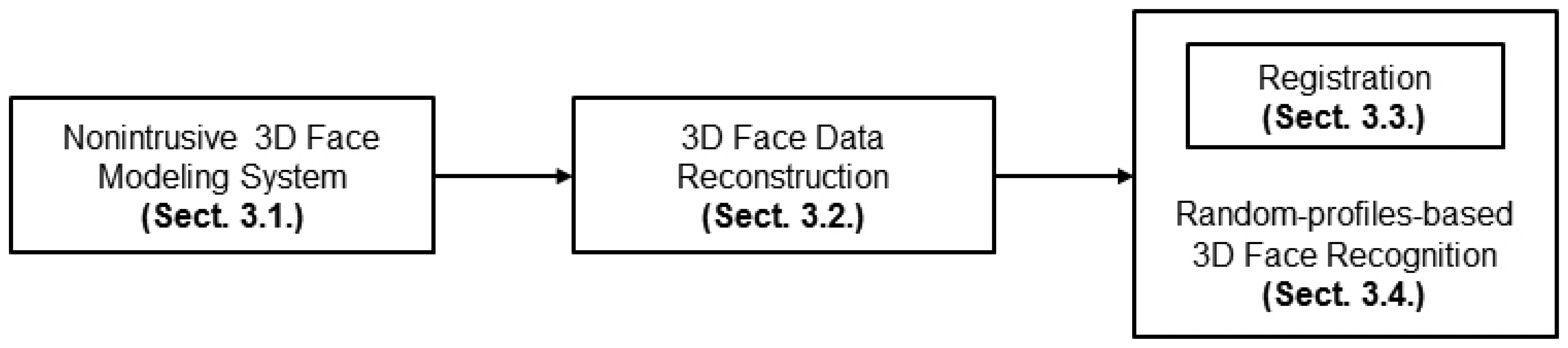
Figure 1 shows an overview of the proposed system. Firstly, the nonintrusive 3D face modeling system, which consists of two cameras and one rotatable NILL, is introduced. Using this system, we perform 3D face data reconstruction to generate not only full-range full-density 3D face data but also precise face profiles for face recognition. The feature-based ICP registration stage is next performed. Finally, we recognize 3D-face-based random profiles.
3.1. Overview of Proposed Nonintrusive 3D Face Modeling System
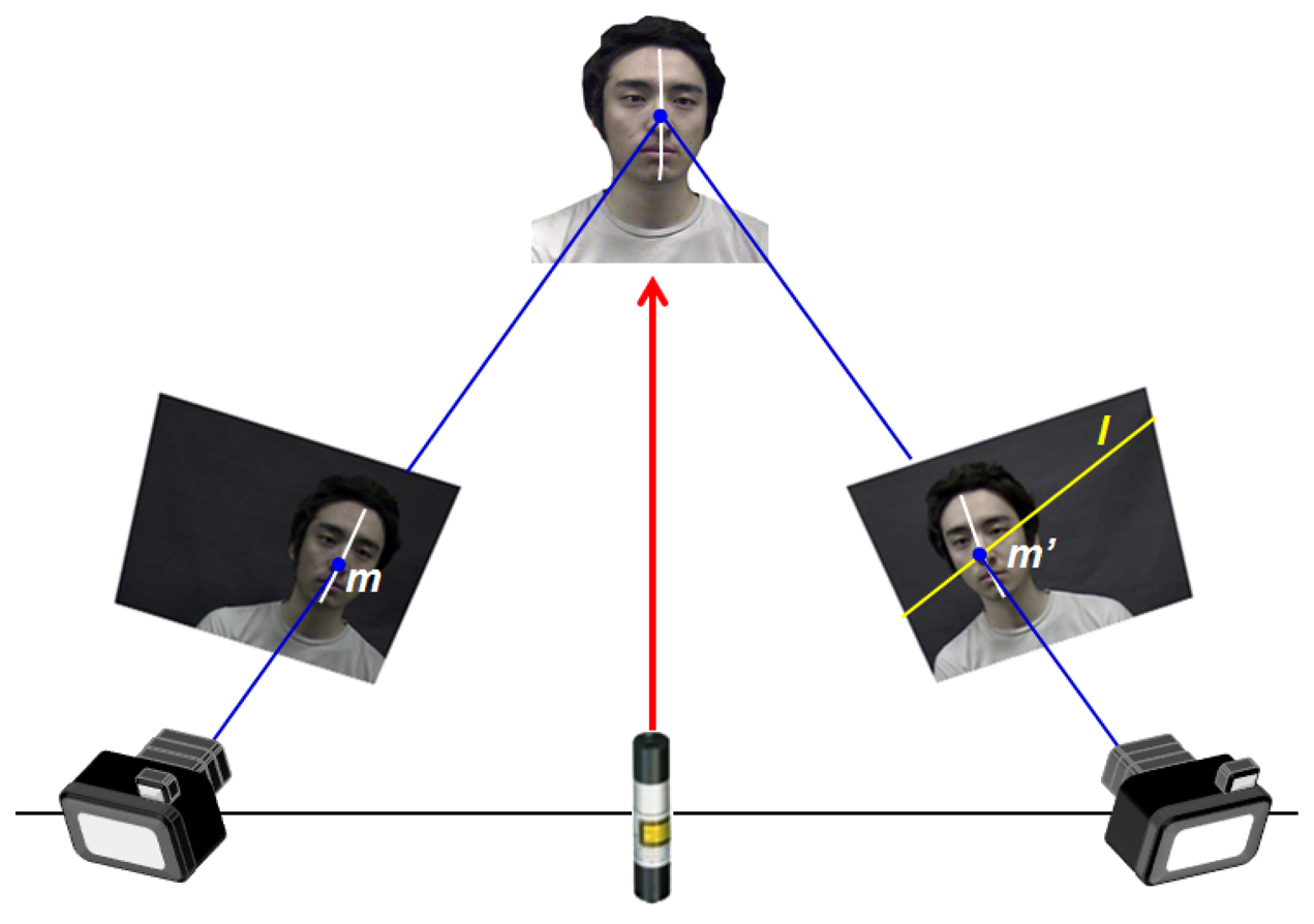
The proposed 3D face modeling system is comprised of two cameras for the stereo vision system and one rotatable NILL. The NILL is located between the two cameras, as shown in Figure 2. The wavelength of the NILL is 850 nm, which is almost invisible to human sight; however, it can be detected by cameras and is safe for human eyes (conforming to IEC 60825-1 Class I Safety) [32]. The cameras, which operate in visible and near-infrared ranges (380nm to 950nm) are used to simultaneously collect the color texture of the face and projected line feature from the NILL. The near-infrared line features projected on the face are represented as a white color in the image; therefore, the performance of 3D reconstruction depends on how well a white line can be extracted. However, it is difficult to accurately extract the line using only image processing techniques because of changes in surrounding illumination. To solve this problem, we use a permeate filter to reduce light reflection and an optical low-pass filter to enhance the visibility of the visible and near-infrared light. After acquiring the images, we extract a line using simple computer vision methods, such as threshold and morphology.
3.2. 3D Face Data Reconstruction
Using multiple images from two cameras, we reconstruct the 3D face data. Figure 3 shows the full process for reconstructing 3D face data. This process is divided into two stages: off-line and on-line processes. In the off-line stage, camera calibration is performed to obtain the intrinsic and extrinsic parameters of two cameras prior to acquiring the images. In addition, the fundamental matrix (F) of Epipolar geometry and projection matrix (P) for 3D reconstruction are then calculated [15].
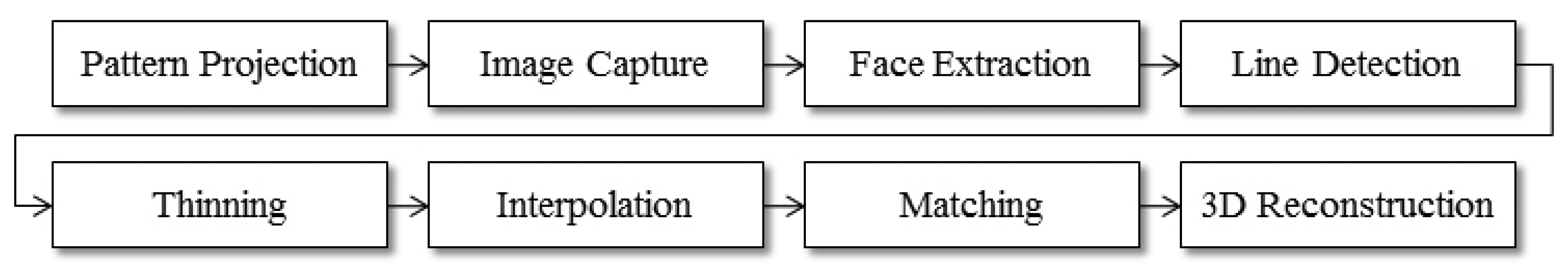
From that point, pattern projection using a NILL, image acquisition, and matching between left and right images, along with the process for 3D reconstruction (such as finding corresponding points and triangulation), are executed during the on-line stage [15]. The on-line stage is substantial for 3D face reconstruction. We further elaborate this stage in detail, as shown in Figure 4.
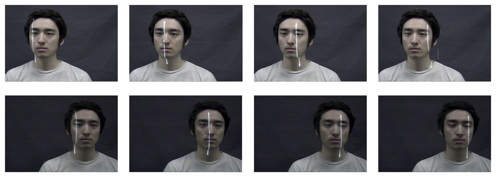
The first step in the on-line process is pattern projection by the NILL. One of three types of patterns-vertical, horizontal, or slant line-can be projected depending on the form of the line pattern. We use vertical patterns because they can reconstruct a 3D face using fewer lines than other forms. The line pattern is projected onto the face to be acquired from left to right at intervals of 5°. Sequential face images are acquired according to the rotation of the NILL by left and right cameras, as shown in Figure 5.
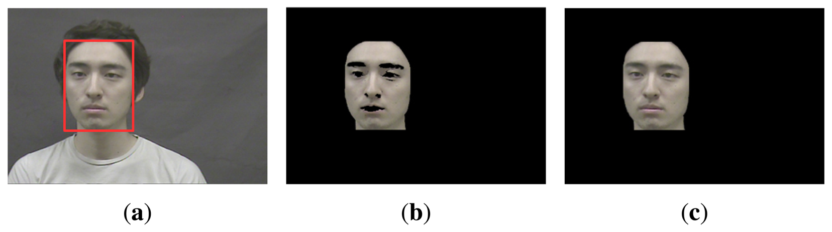
Next, the face region is extracted. This step is essential to speeding up the 3D face data generation by excluding the unwanted regions, such as background and hair. The Viola-Jones object detector is adopted to detect the face region in the left and right images, as shown in Figure 6a [33]. From the detected region, skin color detection in the YCbCr color space −80 ≤ Cr ≤ 120 and 133 ≤ Cb ≤ 165 is performed, as shown in Figure 6b. From that point, morphology operations are performed for noise reduction and hole filling with respect to eye, eyebrows, and so on, as shown in Figure 6c.
We next extract lines projected onto the face. The images are converted into a gray scale image, and we detect a white line using the threshold method in each sequential image. The morphology operation is then applied for noise reduction.
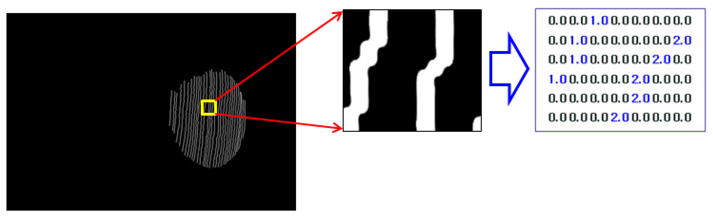
Subsequently, we make the extracted lines thin to find the corresponding point without ambiguity. Codes are generated for each thinned line to separate them. The thinned and coded images are cumulated in an image, as shown in Figure 7.
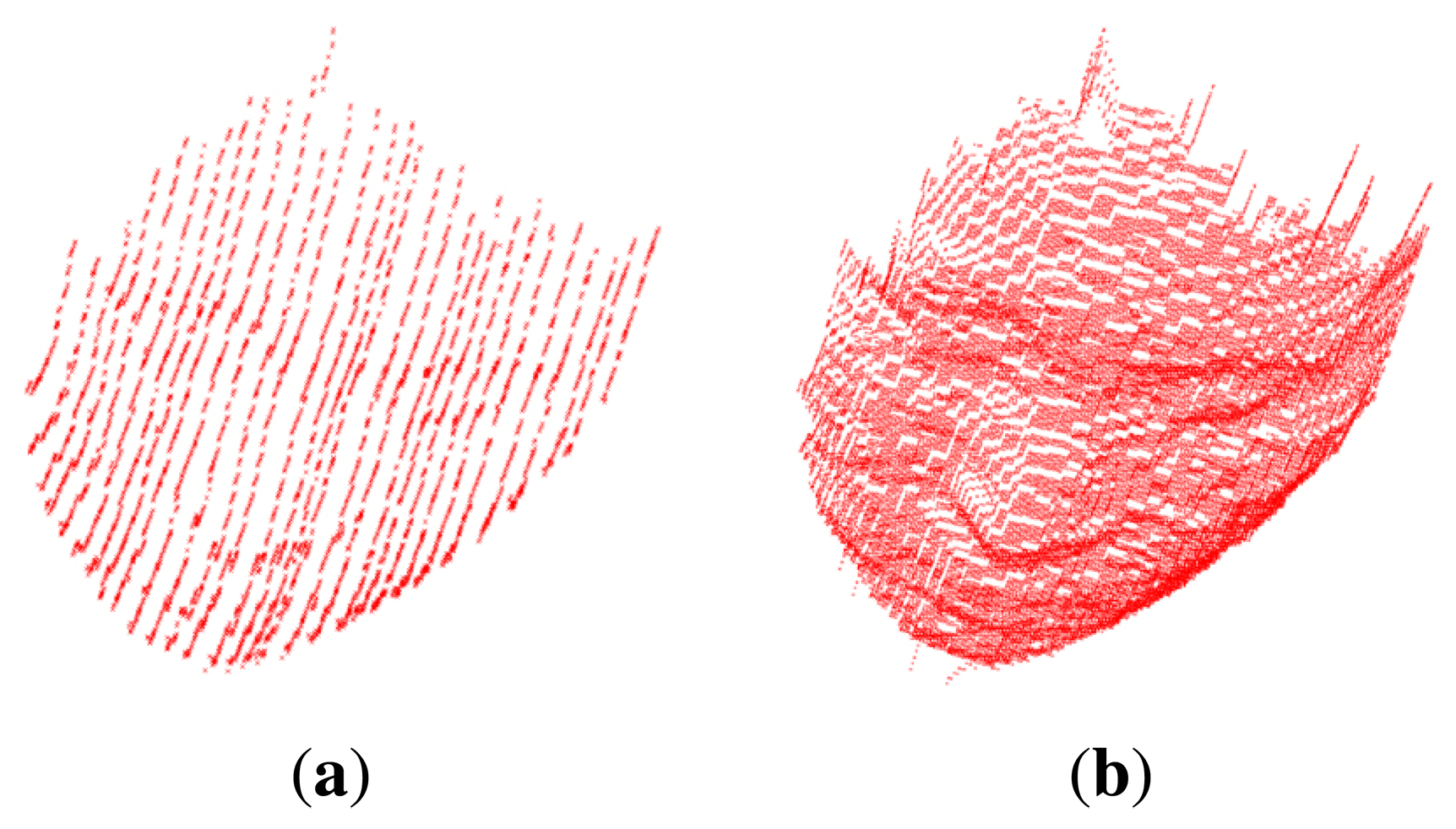
The resultant 3D reconstructed face with thinned lines may be a sparse map; that is, the data in the face image may be sparse between detected lines, as shown in Figure 8a. A dense map, as shown in
Figure 8b, is required for the majority of applications, such as recognition and animation. Therefore, we interpolate the coded empty regions between each coded lines in the 2D image, as shown in Figure 9. We designate the k(x, y) as generated codes of the (x, y) image coordinate:
At this stage, the corresponding points between left and right images are identified using the intersection point of an epipolar line and interpolated coded line about the whole region of the face, as shown in Figure 2. For example, suppose we want to find the correspondence of point (x, y) of the left image in the right image; m̃ is a 2D homogeneous coordinate that appends a 1 to the end of each set of 2D coordinates in the left image:
By using epipolar geometry in a stereo vision system, the correspondence problem becomes a 1D searching problem; that is, the epipolar line (l) is represented by the fundamental matrix (F) as Equation (3) [15]:
If a code on the epipolar line in right image is the same as the k(x, y) in the left image, the correspondence problem is solved. However, the same code may not exist because of the interpolation. Therefore, the most similar code should be found as:
Finally, we reconstruct 3D face data using a triangulation method [15]. The final result is 3D face data in the form of point clouds and color texture.
From the proposed 3D face modeling system, we can acquire three types of data: 2D color image, 3D full-density (FD) data, and 3D profile data. In other words, we can perform three types of face recognition: 2D, which uses 2D face images; 3D FD, and profile-based.
3.3. Registration
Before the face recognition stage, registration is an essential preprocessing step that transforms two different sets of data into the same pose. Poor registration will propagate errors and affect the overall system performance, which particularly impacts profile-based 3D face recognition. In our system, registration is performed in between full-density (FD) 3D face data (gallery) and random profiles (probe), as shown in Figure 10.
The most commonly used algorithm for 3D data registration is the iterative closest point (ICP) [34]. ICP is an iterative procedure that minimizes the mean square error (MSE) between points in one set of data and the closest points in the reference. However, iterative techniques have the disadvantage of being slow (incurring high computational costs) and requiring an initial estimation to begin the iteration.
In terms of the conventional ICP algorithm, the high number of points and large transformation involving rotation R, translation T, and scale s make it operate slowly. In other words, more iterations are required to find each closest point and to calculate the Euclidean distance when the transformation and number of points are large. Because ICP for 3D face recognition uses an especially large number of 3D points, a significant amount of processing time for registration is required. In addition, as with other iterative estimation algorithms, the convergence speed and accuracy of ICP is highly sensitive to the initial estimation; i.e., the initial rotation and translation parameters.
For fast convergence and normalization, we propose a face-feature-based ICP. Through the proposed ICP, we can estimate the initial transformation and normalize the 3D face data. First, face features, such as eyes and lips, are extracted using the active appearance model (AAM) from the 2D gallery and probe image, as shown in Figure 11a [35]. Second, the left and right corners of two eyes and lip position coordinates (6 points) from the 2D face image set are reconstructed into 3D space, as shown in Figure 11b,c. Third, the initial transformation (H) between the gallery and probe is estimated by extracting six 3D points (left and right points of two eyes and lips) as follows:
A simple solution for H can be derived by the direct linear transformation (DLT) algorithm [15]. If we have 6 corresponding points, we then obtain a system of 18 homogenous equations with 16 unknowns. Therefore, we can obtain the least squares solution for the problem by the DLT algorithm.
Using the estimated H matrix, we transform the probe data by the estimated initial transform matrix. Finally, the conventional ICP for the point registration is performed. Table 2 describes the progression of our feature-based ICP.
3.4. Random-Profile-Based 3D Face Recognition
After registration is accomplished, random-profile-based 3D face recognition is performed. In this context, the term “random” means that the number of profiles (from 7 to 12) and the extracted profiles from the face region are arbitrary. The size of the face captured in the image differs based on the distance between the person and the sensor. That is, faces near to the camera are projected as a large size onto the image, while faces that are far from the camera are projected as a small size. The number of profiles that can be extracted from the face region also varies by distance. In addition, based on the persons pose, the size of the face in the image can also change. To increase the flexibility of the proposed system, we apply the concept of “random” to it. Figure 12 illustrates the procedure for our proposed face recognition.
Firstly, the corresponding profiles from the FD 3D gallery of face data are extracted for comparison with the probe random profiles. Figure 13 shows how to extract the corresponding profiles from the FD 3D face data. We derive plane equations from the probe profiles by a normal vector, eigenvector, which is associated with the third largest eigenvalue by singular vector decomposition (SVD), as shown in Figure 13a:
Because we assume that the human face typically has the largest variation in face vertical direction, as shown in Figure 13a, the first eigenvector (υ1) corresponding to the largest eigenvalue represents the vertical direction. On the other hand, the second eigenvector (υ2) direction represents the frontal face direction that has the second largest variation in a profile. When extracting the corresponding profiles from FD 3D face data in the direction of the second eigenvector, we estimate the plane equations of each profile using the third eigenvector (υ3) as a normal vector of the plane equations as shown in Figure 13b. Finally, we find the corresponding profiles as the points intersecting with the planes and FD 3D face data, as shown in Figure 13c. Figure 13d shows the extracted corresponding profiles. In addition, when we extract corresponding profiles from FD 3D face data in the direction of the third eigenvector, we estimate the plane equations of each profile using the second eigenvector as a normal vector of the plane equations.
In addition, we devise an extraction of the corresponding profiles with consideration of the region of the face. As shown in Figure 14a, we divide the face by AAM [35] into two regions: middle (M) and side (S). As a result of AAM, we can obtain the 2D coordinates of landmark points of the face, as shown in the figure. In those points, we denote the S region as the left region of the 7th point and the right region of the 10th point, and the M region as being between the 7th and 10th points. The M region mainly contains the nose, and the S region includes the cheeks. In the M region, the direction of the second eigenvector should best represent the face shape to distinguish different identities. We extract corresponding profiles with respect to the direction of the second eigenvector in the M region. However, we cannot be certain which direction is the most representative for describing the face shape in the S region. Therefore, we compare the performances of using in the S region the direction of the second eigenvector, as shown in Figure 14b, and using the direction of the third eigenvector, as shown in Figure 14c.
After extracting corresponding profiles, we calculate the distance between probe profiles and extracted gallery profiles using the following matching methods:
Average Euclidean Distance (AED) = Total Euclidean Distance/Number of Points
Score Fusion of AED and DTW (AED+DTW).
For the recognition, we first use average Euclidean distance (AED), which is the total Euclidean distance divided by the number of extracted points, because the number of extracted corresponding points can be different according to the probe profiles to be compared. Second, we choose dynamic time warping (DTW) to calculate the similarity of two profiles [36,37]. DTW originally computes the optimal score and finds the optimal alignment between two sequential signals. One DTW-based application is profile-based face recognition [26]. Third, we combine the results of AED and DTW using score fusion. The decision is made based on the smallest difference between the extracted profiles and probe profiles.
4. Experiments
4.1. Experiment Environment
The proposed system consists of two cameras and an 850 nm NILL. For the experiment, we used a 1/3-in Sony IT color CCD image sensor for the cameras and an LTH-30 laser module as the NILL. The cameras were of 704 × 480 resolution and could capture electromagnetic wavelengths from 350 nm to 950 nm in 30 fps. To obtain accurate experimental results, we manually set the camera focus and white balance prior to the test. For temporal synchronization between two cameras, all images were captured with multi-thread technique. Multi-thread technique can capture two images within 1 ms difference. We carried out the experiments with a 3.93 GHz Intel Core i7 870 and 4 G of physical memory.
Figure 15 shows the proposed system and experiment environment. To capture the appropriate number of projected lines onto the face, the distance between the face and system was approximately 1.5 m. To remove the background, we set a dark screen behind the person whose face was to be acquired.
4.2. 3D Face Reconstruction
We reconstructed 3D face data consisting of more than 50,000 3D points by using the proposed system. Processing time was about 3 seconds for more than 50,000 3D points reconstruction, as shown in Figure 16, including image acquisition time.
To verify our proposed recognition method with this system, we created a database consisting of 50 subjects, as shown in Figure 17. First, we created FD 3D face data of 50 subjects with a frontal pose, which served as gallery data, as shown in Figure 18a. Second, we extracted random profiles from 50 subjects in 5 different poses-frontal, left, right, up, and down-as probe data (Figure 18b). The number of profiles for each probe was randomly selected from 7 to 12. Those selected profiles contained the whole region of the face, not a specific region within it.
4.3. Registration
To compare the proposed feature-based ICP with conventional ICP, we recorded the number of iterations of two methods for convergence. The partial random profiles consisting of 50 subjects in 5 poses (250 total) were used as the probe profiles. The FD 3D face data as gallery data was used for the ICP algorithm. Table 3 shows the comparison result in terms of number of iterations according to different poses.
The number of iterations was calculated by averaging the number of iterations that converged partial random profiles into frontal full 3D face data. As a result of the comparison, the average number of iterations of the proposed ICP was 29.489 and that of the conventional ICP was 77.072. The experiment result shows that the proposed ICP is approximately 3 times faster than the conventional ICP. Figure 19 shows the result of the registration. Before the registration, the profiles (red) and FD 3D face data (blue) were quite wrenched, as shown in Figure 19a. However, they were aligned after registration, as depicted in Figure 19b.
4.4. Random-Profile-Based 3D Face Recognition
To evaluate the proposed random-profile-based 3D face recognition, we created FD 3D face data of 50 subjects in a frontal pose, which served as gallery data. We also generated as probe data 3D random profiles from 50 subjects in 5 different poses: frontal, left, right, up, and down. Because we randomly extracted the same profiles from 7 to 12 as gallery data, each data consisted of a different number of profiles. Table 4 shows the number of data according to the number of profiles. Also, Table 5 shows the number of data according to the regions of face. (left side, right side and middle region of face). In addition, we created 2D face data of 50 subjects in 5 poses for 2D face recognition.
We performed three experiments to evaluate the proposed methods as listed below:
Evaluation according to the regions of the face.
Comparison of recognition rate between proposed system and other methods.
Fusion of 3D face recognition and 2D face recognition.
4.4.1. Performance Evaluation Based on Face Region
Firstly, using FD 3D face data and random profiles, we compared the performances based on regions of the face, which were divided into middle (M) and side (S) regions. Table 6 shows the recognition rates according to the region of the face. The result shows that the middle (M) region of the face has more discriminant features than the side (S) region. In addition, the recognition rate using random profiles extracted by the second eigenvector direction was slightly higher than the recognition rate using random profiles extracted by the third eigenvector direction. As showns in Figure 20, the result using middle region of face shows the better performance than the result using side region of face.
4.4.2. Performance Comparision with 2D Face Recognition
To verify the proposed system, we compared our proposed method with well-known 2D face recognition methods as follows:
Principal component analysis (PCA) [38]
Fisher linear discriminant analysis (FLDA) [39]
PCA feature extraction + support vector machine (PCA+SVM) [40,41]
PCA feature extraction + reduced multivariate polynomial pattern classifier (PCA+RM) [42,43]
We performed five-fold cross-validation to verify 2D face images that were normalized by a 56×46 size. That is, four face images of a subject were used for training and were then employed on the face image used for testing. The parameters, such as the number of principal components in the eigenface and number of support vectors with SVM, were experimentally selected to achieve the lowest error rate by each method. In the PCA+RM experiment, as polynomial order 3 showed saturated performance, the experimental result was obtained with order 3. Table 7 shows the results of a comparison between the proposed method and 2D face recognition.
Based on the experimental results, the recognition rates of AED-based recognition were 81.2%a and 82.0%d by using the second eigenvector direction, and second and third eigenvector directions, respectively. The recognition rates of DTW-based recognition were 84.8%b and 85.6%e by using the second eigenvector direction, and second and third eigenvector directions, respectively. The DTW-based recognition showed a better recognition rate than AED-based. The recognition rates of AED+DTW-based recognition were 88.0%c and 89.6%f by using the second eigenvector direction, and second and third eigenvector directions, respectively. The recognition rate by PCA, FLDA, SVM and RM were 66%g, 73.2%h, 77.6%i and 76.4%j, respectively.
As shown in Figure 21, the proposed recognition method showed better performance against pose variation than other 2D-based methods. Even though the recognition rate using the second eigenvector direction was similar to the face recognition rate using the second and third eigenvector directions, the recognition rate using the second and third eigenvector directions was slightly higher than that of the second eigenvector direction. In addition, among the proposed recognition methods, the score fusion of AED and DTW demonstrated the best performance.
4.4.3. Fusion of Proposed 3D Face Recognition and 2D Face Recognition
Although the recognition rate of the proposed random-profile-based 3D face recognition was higher than 2D face recognition under pose variation, we nevertheless fused the results of the proposed 3D face recognition and 2D face recognition to enhance the recognition rate. Table 8 shows the fusion results. The first row represents the result of fusion between random-profile-based 3D face recognition using only the second eigenvector direction and 2D face recognition, such PCA, FLDA, PCA + SVM and PCA + RM. The second row was the result of fusion between the proposed face recognition using random profiles extracted by the second and third eigenvector directions and 2D face recognition.
By fusing the results of 3D and 2D face recognition, the overall recognition rates were greater than the recognition rate by single face recognition. The fusion of AED + DTW as 3D face recognition and PCA + SVM as 2D face recognition showed the best performance among the various experimental results. Moreover, these experimental results showed good performance under pose variation, which is one of the most significant factors to cause performance reduction in face recognition.
5. Conclusions
In this paper, we proposed a novel 3D face acquisition and recognition system. The 3D face data acquisition system is based on a stereo vision system and an invisible line laser as a projection feature. The 3D face recognition system is based on randomly extracted profiles. Through the proposed acquisition system, we reconstructed 3D face data composed of more than 50,000 3D points. In addition, we proposed a novel 3D face recognition method based on random profiles.
The proposed recognition method uses random profiles directly reconstructed by the proposed 3D face acquisition system, not by full density (FD) 3D face data. Therefore, it is memory efficient and requires lower computational costs than the system using FD 3D face data. The experiment results demonstrated that the proposed system can produce accurate 3D face data with simple line patterns, and achieves robust recognition performance against pose variation.
Acknowledgments
This work was supported by a National Research Foundation of Korea (NRF) grant funded by the Korean government (MEST) (NRF-2011-0016302). Additionally, this research was supported by the MSIP (Ministry of Science, ICT and Future Planning), Korea, under the ITRC (Information Technology Research Center) support program (NIPA-2014-H0301-14-1012) supervised by the NIPA (National IT Industry Promotion Agency).
References
- O'Gorman, L. Comparing passwords, tokens, and biometrics for user authentication. Proc. IEEE 2003, 91, 2019–2040. [Google Scholar]
- Zhao, W.; Chellappa, R.; Phillips, P.J.; Rosenfeld, A. Face recognition: A literature survey. ACM Comput. Surv. (CSUR) 2003, 35, 399–458. [Google Scholar]
- Qin, H.; Qin, L.; Xue, L.; Li, Y. Kernel Gabor-Based Weighted Region Covariance Matrix for Face Recognition. Sensors 2012, 12, 7410–7422. [Google Scholar]
- Klare, B.F.; Burge, M.J.; Klontz, J.C.; Vorder Bruegge, R.W.; Jain, A.K. Face Recognition Performance: Role of Demographic Information. IEEE Trans. Inf. Forensics Secur. 2012, 7, 1789–1801. [Google Scholar]
- Bowyer, K.W.; Chang, K.; Flynn, P. A survey of approaches to three-dimensional face recognition. Pattern Recognit. 2004, 1, 358–361. [Google Scholar]
- Malassiotis, S.; Strintzis, M.G. Pose and illumination compensation for 3D face recognition. Int. Conf. Image Process. 2004, 1, 91–94. [Google Scholar]
- Malassiotis, S.; Strintzis, M.G. Robust Face Recognition Using 2D and 3D Data: Pose and Illumination Compensation. Pattern Recognit. 2005, 38, 2537–2548. [Google Scholar]
- Abatea, A.F.; Nappi, M. Daniel Riccioa and Gabriele Sabatinoa, 2D and 3D face recognition: A survey. Pattern Recognit. Lett. 2007, 28, 1885–1906. [Google Scholar]
- Smeets, D.; Claes, P.; Hermans, J.; Vandermeulen, D.; Suetens, P. A Comparative Study of 3D Face Recognition Under Expression Variations. IEEE Trans. Syst. Man Cybern. Part C: Appl. Rev. 2012, 42, 710–727. [Google Scholar]
- Uchida, N.; Shibahara, T.; Aoki, T.; Nakajima, H.; Kobayashi, K. 3D face recognition using passive stereo vision. Image Process. 2005, 2, 950–953. [Google Scholar]
- Jin, S.; Cho, J.; Pham, X.D.; Lee, K.M.; Park, S.-K.; Kim, M.; Jeon, J.W. FPGA Design and Implementation of a Real-Time Stereo Vision System. Circuits Syst. Video Technol. 2010, 20, 15–26. [Google Scholar]
- Scharstein, D.; Szeliski, R. High-accuracy stereo depth maps using structured light. Comput. Vision Pattern Recognit. 2003, 1, I:195–I:202. [Google Scholar]
- Chen, S.Y.; Li, Y.F.; Zhang, J. Vision Processing for Realtime 3D Data Acquisition Based on Coded Structured Light. IEEE Trans. Image Process. 2008, 17, 167–176. [Google Scholar]
- Konica Minolta. Available online: http://www.konicaminolta.com/instruments/download/instruction_manual/3d/ (accessed on 29 March 2014).
- Hartley, R.; Zisserman, A. Multiple View Geometry; Cambridge University Press: Cambridge, UK, 2000. [Google Scholar]
- Blanz, V.; Romdhani, S.; Vetter, T. Face Identification across Different Poses and Illuminations with a 3D Morphable Model. Proceedings of the 5th IEEE Conference on Automatic Face and Gesture Recognition, Washington, DC, USA, 20–21 May 2002; pp. 202–207.
- Kim, J.; Yu, S.; Hwang, J.; Sooyeon, K.; Sangyoun, L. Nonintrusive 3-D face data acquisition system. Proceedings of the 4th IEEE Conference on Industrial Electronics and Applications, Xi'an, China, 25–27 May 2009; pp. 642–646.
- Kolb, A.; Barth, E.; Koch, R.; Larsen, R. Time-of-Flight Sensors in Computer Graphics. Eurographics Star Report 2009. [Google Scholar]
- Kinect. Available online: http://en.wikipedia.org/wiki/Kinect (accessed on 29 March 2014).
- Pan, G.; Wu, Z. 3D Face Recognition From Range Data. Int. J. Image Gr. 2005, 5, 573–593. [Google Scholar]
- Achermann, B.; Jiang, X.; Bunke, H. Face recognition using range images. Proceedings of the International Conference on Virtual Systems and MultiMedia, Geneva, The Switzerland, 10–12 September 1997; pp. 129–136.
- Lee, Y.; Park, K.; Shim, J.; Yi, T. 3D face recognition using statistical multiple features for the local depth information. Proceedings of the 17th ICVI, Halifax, Canada, 11–13 June 2003.
- Gordon, G. Face recognition based on depth and curvature features. Geom. Methods Comput. Vis. 1991, 1570, 234–247. [Google Scholar]
- Tanaka, H.; Ikeda, M.; Chiaki, H. Curvature-based face surface recognition using spherical correlation. proceedings of the Third IEEE International Conference on Automatic Face and Gesture Recognition, Nara, Japan, 14–16 April 1998; pp. 372–377.
- Li, C.; Barreto, A. Profile-Based 3D Face Registration and Recognition. Lect. Notes Comput. Sci. 2005, 3506, 478–488. [Google Scholar]
- Bhanu, B.; Zhou, X. Face recognition from face profile using dynamic time warping. Proceedings of the 17th International Conference on the Pattern Recognition, Cambridge, UK, 23–26 August 2004; pp. 499–502.
- Beumier, C.; Acheroy, M. Automatic 3D face authentication. Image Vis. Comput. 2001, 18, 315–321. [Google Scholar]
- Berretti, S.; Del Bimbo, A.; Pala, P. 3D Face Recognition Using Isogeodesic Stripes. IEEE Trans. Pattern Anal. Mach. Intell. 2010, 32, 2162–2177. [Google Scholar]
- Pan, G.; Wu, Y.; Wu, Z.; Liu, W. 3D Face Recognition by Profile and Surface Matching. Proceedings of the International Joint Conference on Neural Networks, Portland, OR, USA, 20–24 July 2003; pp. 2169–2174.
- Tang, H.; Sun, Y.; Baocai, Y.; Yun, G. 3D Face Recognition Based on Facial Profiles. proceedings of the International Conference on Information Engineering and Computer Science, Wuhan, China, 19–20 December 2009; pp. 1–5.
- Efraty, B.A.; Ismailov, E.; Shah, S.; Kakadiaris, I.A. Towards 3D-aided Prole-Based Face Recognition. proceedings of the 16th IEEE International Conference on Image Processing, Washington, DC, USA, 28–30 September 2009; pp. 1–8.
- IEC 60825-1: Safety of laser products—Part 1: Equipment classification and requirements, 2nd ed.; International Electrotechnical Commission: Geneva, Switzerland, 2007.
- Viola, P.; Jones, M.J. Rapid Object Detection using a Boosted Cascade of Simple Features. Proceedings of the 2001 IEEE Computer Society Conference on Computer Vision and Pattern Recognition, Kauai, HI, USA, 8–14 December 2001; pp. I-511–I-518.
- Besl, P.J.; McKay, N.D. A method for registration of 3d shapes. IEEE Trans. Pattern Anal. Mach. Intell. 1992, 14, 239–256. [Google Scholar]
- Cootes, T.F.; Edwards, G.; Taylor, C. Active Appearance Models. IEEE Trans. Pattern Anal. Mach. Intell. 2001, 23, 681–685. [Google Scholar]
- Sakoe, H.; Chiba, S. A dynamic programming approach to continuous speech recognition. Int. Cong. Acoust. 1971, 3, 65–69. [Google Scholar]
- Itakura, F.I. Minimum prediction residual principle applied to speech recognition. IEEE Trans. Acoust. Speech Signal Process. 1975, 23, 67–72. [Google Scholar]
- Turk, M.; Pentland, A. Eigenface for recognition. J. Cogn. Neurosci. 1991, 3, 71–86. [Google Scholar]
- Lu, J.; Plataniotis, K.N.; Venetsanopoulos, A.N. Face recognition using LDA-based algorithms. IEEE Trans. Neural Netw. 2003, 14, 195–200. [Google Scholar]
- Faruqe, M.O.; Mehedi, A.l.; Hasan, M. Face recognition using PCA and SVM. proceedings of the 3rd International Conference on Anti-counterfeiting, Security, and Identification in Communication, Hong Kong, China, 20–22 August 2009; pp. 97–101.
- Li, J.; Zhao, B.; Zhang, H.; Jiao, J. Face Recognition System Using SVM Classifier and Feature Extraction by PCA and LDA Combination. proceedings of the International Conference on Computational Intelligence and Software Engineering, Wuhan, China, 11–13 December 2009; pp. 1–4.
- Toh, K.-A.; Tran, Q.-L.; Srinivasan, D. Benchmarking a Reduced Multivariate Polynomial Pattern Classifier. Pattern Anal. Mach. Intell. 2004, 26, 740–755. [Google Scholar]
- Oh, B.-S.; Toh, K.-A.; Choi, K.; Jin Teoh, A.B.; Kim, J. Extraction and fusion of partial face features for cancelable identity verification. Pattern Recognit. 2012, 45, 3288–3303. [Google Scholar]


| System | LS | SVS | SLS |
|---|---|---|---|
| Price | High | Low | Medium |
| Scan Time | Slow | Fast | Fast |
| Accuracy | High | Low | High |
| Aversion | High | Low | High |
|
| Pose of profiles | General ICP | Proposed ICP |
|---|---|---|
| Frontal | 69.12 | 27.49 |
| Left | 77.88 | 29.23 |
| Right | 83.6 | 30.53 |
| Up | 75.28 | 30.37 |
| Down | 79.48 | 29.87 |
| Average | 77.072 | 29.498 |
| # of profiles | 7 | 8 | 9 | 10 | 11 | 12 |
|---|---|---|---|---|---|---|
| # of data | (37/250) | (41/250) | (48/250) | (45/250) | (39/250) | (40/250) |
| Region of face | left side | middle | right side |
|---|---|---|---|
| # of data | (53/250) | (146/250) | (51/250) |
| Middle (M) Region | Side (S) Region | |||||||
|---|---|---|---|---|---|---|---|---|
| AED | DTW | AED + DTW | 2nd eigenvector based | 2nd and 3rd eigenvector based | ||||
| AED | DTW | AED + DTW | AED | DTW | AED + DTW | |||
| 78.4% | 82.4% | 84.4% | 66% | 71.2% | 73.2% | 66.8% | 72.4% | 75.6% |
| (196/250) | (206/250) | (211/250) | (165/250) | (178/250) | (183/250) | (167/250) | (181/250) | (189/250) |
| Proposed Random-profile-based recognition | 2D Face Recognition | ||||||||
|---|---|---|---|---|---|---|---|---|---|
| 2nd eigenvector based | 2nd and 3rd eigenector based | PCAg | FLDAh | PCA+SVMi | PCA+RMj | ||||
| AEDa | DTWb | AED+DTWc | AEDd | DTWe | AED+DTWf | ||||
| 81.2%(203/250) | 84.8%(212/250) | 88.0%(220/250) | 82.0%(205/250) | 85.6% (214/250) | 89.6%(224/250) | 66% (165/250) | 73.2% (183/250) | 77.6% (194/250) | 76.4% (191/250) |
| 2nd eigenvector based | 2nd and 3rd eigenvector based | |||||||
|---|---|---|---|---|---|---|---|---|
| PCA | FLDA | PCA+SVM | PCA+RM | PCA | FLDA | PCA+SVM | PCA+RM | |
| AED | 84.4% (211/250) | 87.2% (218/250) | 90.8% (227/250) | 88.4% (221/250) | 84.8% (212/250) | 88.4% (221/250) | 91.6% (229/250) | 89.2% (223/250) |
| DTW | 85.6% (214/250) | 88.0% (220/250) | 92.4% (231/250) | 90% (225/250) | 82.0% (216/250) | 86.4% (224/250) | 89.6% (235/250) | 90.8% (227/250) |
| AED+DTW | 87.6% (219/250) | 89.2% (223/250) | 93.6%(234/250) | 90.8% (227/250) | 88.4% (221/250) | 90.4% (226/250) | 94.8%(237/250) | 92.4% (231/250) |
© 2014 by the authors; licensee MDPI, Basel, Switzerland. This article is an open access article distributed under the terms and conditions of the Creative Commons Attribution license ( http://creativecommons.Org/licenses/by/3.0/).
Share and Cite
Kim, J.; Yu, S.; Lee, S. Random-Profiles-Based 3D Face Recognition System. Sensors 2014, 14, 6279-6301. https://doi.org/10.3390/s140406279
Kim J, Yu S, Lee S. Random-Profiles-Based 3D Face Recognition System. Sensors. 2014; 14(4):6279-6301. https://doi.org/10.3390/s140406279
Chicago/Turabian StyleKim, Joongrock, Sunjin Yu, and Sangyoun Lee. 2014. "Random-Profiles-Based 3D Face Recognition System" Sensors 14, no. 4: 6279-6301. https://doi.org/10.3390/s140406279