A Class of Coning Algorithms Based on a Half-Compressed Structure


Abstract
: Aiming to advance the coning algorithm performance of strapdown inertial navigation systems, a new half-compressed coning correction structure is presented. The half-compressed algorithm structure is analytically proven to be equivalent to the traditional compressed structure under coning environments. The half-compressed algorithm coefficients allow direct configuration from traditional compressed algorithm coefficients. A type of algorithm error model is defined for coning algorithm performance evaluation under maneuver environment conditions. Like previous uncompressed algorithms, the half-compressed algorithm has improved maneuver accuracy and retained coning accuracy compared with its corresponding compressed algorithm. Compared with prior uncompressed algorithms, the formula for the new algorithm coefficients is simpler.1. Introduction
In the recent decades since Jordan [1] and Bortz [2] introduced the two-stage attitude updating algorithm for strapdown inertial navigation systems (SINS), the design of efficient coning algorithms which include designing an efficient coning correction structure and achieving the optimized structure coefficients for coning correction accounting for a portion of the rotation vector has always been an attractive topic.
Jordan [1] first presented the two-sample algorithm structure for non-commutativity error compensation. Miller [3] first presented the three-sample algorithm structure and the concept of designing the coning correction algorithm for optimum performance in a pure coning environment by using a truncated coning frequency Taylor-series expansion formulation for updating the rotation vector errors corresponding to updating the quaternion error. On the basis of Miller's idea, Ignagni [4] summarized the generally uncompressed algorithm structure for coning correction and proposed several coning correction algorithms. Lee [5] applied Miller's idea and concluded that there exists redundancy in the uncompressed coning correction structure under coning motion conditions. Based on Lee's conclusion, Ignagni [6] proved that the cross product of both integral angular rate samples is independent of absolute time and a function of merely the relative time interval between sampling points under coning motion conditions, and derived the first compressed coning correction structure. Different from the previous coning algorithms for gyro error-free outputs, Mark [7] disclosed a method of tuning high-order coning algorithms to match the frequency response characteristics of gyros with filtered outputs. Based on the compressed coning correction structure, Savage [8] further expanded Miller's idea, and raised an idea of using the least square method to design the coning correction algorithm for balanced coning performance in a given discrete coning environment. Song [9] concentrated on the improvement of maneuver accuracy of coning algorithms, and developed an approach for recovering maneuver accuracy in previous coning algorithms based on the uncompressed structure by combining the earliest time Taylor-series method and the latest frequency methods.
This paper proposes a new half-compressed coning correction structure which is analytically proven to be equivalent to the traditional compressed coning correction structure under coning motion conditions. On the basis of the equivalency of the two types of structures, the half-compressed algorithm coefficients can be derived directly from the past compressed coning algorithm coefficients, rather than being specifically designed for coning or maneuver environments. The building of a reasonable structure makes for a simpler formula for the coefficients, retained coning accuracy and improved maneuver performance for the new half-compressed algorithm.
2. Attitude Algorithm Structure
The classical attitude updating computation formula [1,2,8] in modern strapdown inertial navigation systems is given by:
3. Coning Correction Structure
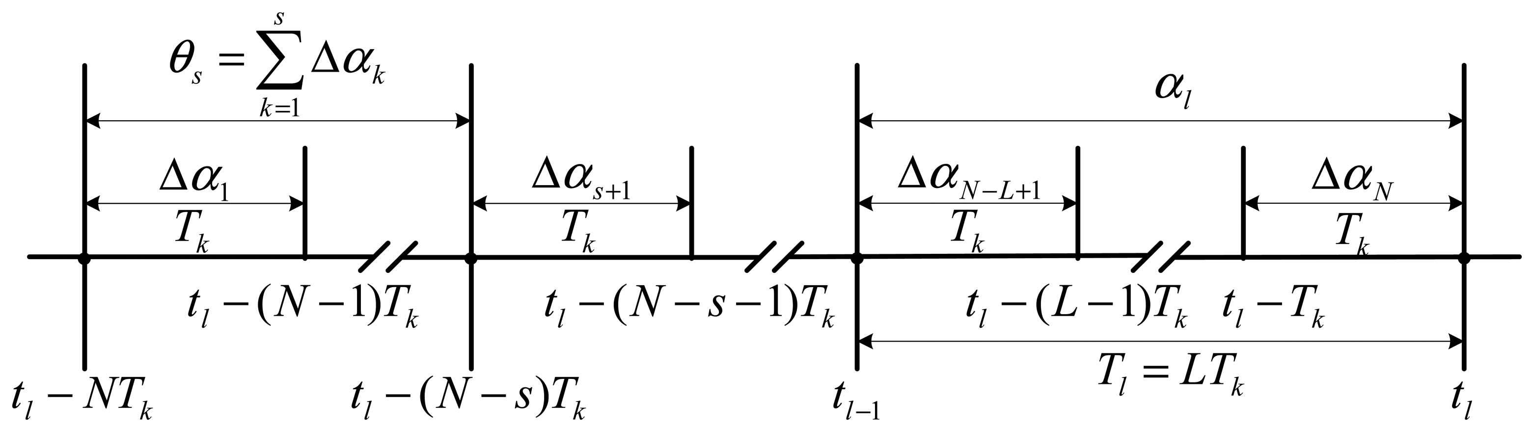
In recent decades, strapdown attitude algorithm design activity has centered on developing routines for computing the coning correction using various approximations to the updating rotation vector ϕl in Equation (2). The traditional numerical computation algorithm formula for updating rotation vector ϕl has the form of the integrated angular rate αl and the coning correction [4,6,8,9]:
Based on the pure coning motion properties, the compressed algorithm form [6,8] equivalent to the uncompressed form for the coning correction in Equation (3) is given by:
Both traditional coning correction forms defined by Equations (3) and (4) are equivalent under coning motion conditions, but not equivalent under maneuver conditions. Song [9] indicated that the algorithms based on the uncompressed form of Equation (3) would give much higher maneuver accuracies, but have a much heavier computation load than those based on the compressed form of Equation (4) after intensive design under maneuver conditions. This paper proposes a half-compressed algorithm form different from the former forms for coning correction given by:
4. Coning Correction Structure Equivalency and Algorithm Design
Assume that the body is undergoing the pure coning motion defined by the angular rate vector [4,6,8]:
Under the coning motion defined by Equation (6), Ignagni [4] had derived the cross product Δαi × Δαj:
Simplification of the coning algorithm form of Equation (3) in the form of Equation (4) in [6], utilizing the coning property expressed by Equation (7) also allows the coning algorithm form of Equation (5) to be simplified as the form of Equation (4) with the relationship of coefficients Js s and Ks s:
It is easily proved that CN−1 is a non-singular matrix. Thus A and B are linear representation. That means, N-sample coning algorithms designed by using the same optimum method and based on the correction structures of Equation (4) and Equation (5) have the same coning correction value under pure a coning motion. Therefore, Equation (5) and Equation (4) are equivalent under coning motions. Solving Equation (8) results in:
5. Algorithm Performance Evaluation
Above we have verified that the half-compressed structure of Equation (5) and the compressed structure of Equation (4) are equivalent under pure coning motion. The uncompressed algorithm based on Equation (3) presented by Song [9] also has the same accuracy as the compressed algorithm based on Equation (4) under a coning motion. Thus, the algorithms designed by using the same optimum method and based on Equations (3)–Equation (5) have the same coning correction accuracy under a pure coning environment.
Below is an error model used for evaluating the coning algorithm accuracy under maneuver environments. Assume that the body is undergoing a maneuver angular motion characterized by the angular rate vector:
Through investigating Equation (10) and Equation (11), we can get the relationship of gj s and ḡj s:
According to the maneuver error analysis method given by [9], the error of a coning algorithm based on uncompressed correction structure of Equation (3) under the maneuver motion expressed by Equation (11) with M ≥ 5 can be built as:
According to Equations (3)–(5), Equation (13) can be used for analyzing the maneuver errors of coning algorithms based on the compressed correction structure of Equation (4) and the half-compressed correction structure of Equation (5), when the coefficients K s in Equation (4) and the coefficients J s in Equation (5) are respectively expanded into the coefficients ς s in Equation (3) with the following relationships:
6. Algorithm Examples and Simulation
To illustrate the properties of coning algorithms, algorithm errors computed using the optimized coning correction coefficients designed by using the frequency Taylor-series method and least minimum square method would be produced, compared, and analyzed under coning environments and maneuver environments, each with Tk = 0.001s, Tl = LTk and L = N:
- (1)
FTSc indicates the coning algorithm based on the compressed form of Equation (4) taking the coefficients designed by using frequency Taylor-series method.
- (2)
LMSc indicates the coning algorithm based on the compressed form of Equation (4) taking the coefficients designed by using least minimum square method.
- (3)
FTShc indicates the coning algorithm based on the half-compressed form of Equation (5) taking the coefficients designed by using frequency Taylor-series method.
- (4)
LMShc indicates the coning algorithm based on the half-compressed form of Equation (5) taking the coefficients designed by using least minimum square method.
- (5)
FTSuc indicates the coning algorithm based on the uncompressed form of Equation (3) taking the coefficients designed by Song [9] using frequency Taylor-series method.
- (6)
LMSuc indicates the coning algorithm based on the uncompressed form of Equation (3) taking the coefficients designed by Song [9] using least minimum square method.
- (7)
X-N indicates the N-sample algorithm X (X respectively denote FTSc, LMSc, FTShc, LMShc, FTSuc and LMSuc).
Tables 1 and 2 respectively give the 3-to-5-sample FTSc and LMSc algorithm coefficients Ks s [5,6,8,9]. Using Equation (9), we can obtain the 3-to-5-sample FTShc and LMShc algorithm coefficients Js s given in Tables 3 and 4 from coefficients Ks s in Tables 1 and 2. According to Equation (15), expanding the coefficients Ks s in Tables 1 and 2 give the expanded coefficients ς s in Tables 5 and 6 for maneuver accuracy evaluation. According to Equation (16), expanding the coefficients Js s in Tables 3 and 4 give the expanded coefficients ς s in Tables 7 and 8 for maneuver accuracy evaluation.
Tables 9 and 10 give the 3-to-5-sample FTSuc and LMSuc algorithm coefficients ς s designed by Song [9] from the coefficients Ks s in Tables 1 and 2, respectively.
The coefficients z3, z4, z51, z52, z61, z62, z71, z72 and z73 depending on the power series terms in Equation (13) are calculated with the coefficients in Tables 5, 6, 7, 8, 9 and 10, and respectively listed in Tables 11, 12, 13, 14, 15 and 16.
The maneuver environment set for algorithm accuracy evaluation is the extreme 2 s angular rate profile pictured in Figure 2 with M = 5, = [0 0 0]T, = [19572/143 −4360/143 −21800/143]T, = [1007/41 4000/143 9369/67]T, = [4843/155 −4000/117 −9206/213]T and = [−5813/131 − 625/858 3258/281]T in Equation (10). The dimension is deg/s for s. According to Equation (13), the maneuver error vector em (t) is computed for the compressed algorithms, the half-compressed algorithms and the uncompressed algorithms with Tables 5, 6, 7, 8, 9 and 10 coefficients over the Figure 2 maneuver profile.
Accordingly, maximum maneuver errors of several concerned algorithms over 2 s maneuver are listed in Table 17.
Comparing the data in Tables 11 to 16, it is indicated that the absolute values of z3 for FTSc, FTShc and FTSuc algorithms are zeros, LMSc, LMShc and LMSuc algorithms have the same non-zero z3, the absolute values of z4 for 3 to 5 sample FTShc (or LMShc) algorithms are respectively about one third, one sixth and one tenth those of z4 for 3 to 5 sample FTSc (or LMSc) algorithms, while the absolute values of z4 for 3 to 5 sample FTSuc (or LMSuc) algorithms are much smaller than those for 3 to 5 sample FTShc (or LMShc) algorithms. If the low order term with z in Equation (13) is the main supply of maneuver error, it would be concluded that the maneuver accuracy of FTShc algorithm is higher than that of FTSc algorithm if the FTSuc algorithm is compared with the FTShc algorithm, and the maneuver accuracy of LMShc algorithm is higher than that of LMSc algorithm if the LMSuc algorithm is compared with LMShc algorithm ignoring the error term with z3. The simulation results in Table 17 are basically consistent with the analytical conclusion above, whereas the maximum maneuver error of the LMSuc3 algorithm is bigger than that of the LMSc3 and LMShc3 algorithms owing to the coupling of the first two error terms with z3 and z4 under this particular 2 s maneuver condition.
According to the 21.3 μrad error contribution from sensors in Table 2 of [8] during the similar maneuver environment, all concerned algorithms with the maximum errors in Table 17 contributing less than 1% of 10 to 20 μrad are compatible with the overall INS accuracy requirement of 0.01 deg/h. Like the uncompressed algorithm (reference [9]), the half-compressed algorithm has significantly more accuracy than the past compressed algorithm, and the new algorithm is more than adequate for modern INS applications. The formula for the algorithm coefficients for the new half-compressed algorithm is simpler compared to the uncompressed algorithm.
7. Conclusions
The new half-compressed coning algorithm can be directly derived from the past compressed coning algorithm. The new algorithms are highly efficient overall in coning and maneuver environments. Compared with the past uncompressed algorithm, the formula for the new algorithm coefficients is simpler. Like the past uncompressed algorithm, the half-compressed algorithm and its corresponding compressed algorithm have the same coning accuracy, while the maneuver accuracy of the half-compressed algorithm is significantly higher than the past compressed algorithm, and more than adequate for modern INS applications.
Acknowledgments
This work was supported in part by the National Natural Science Foundation of China (No. 51375087), the Specialized Research Fund for the Doctoral Program of Higher Education (No. 20110092110039), the Ocean Special Funds for Scientific Research on Public Causes (No. 201205035-09), the Scientific Research Foundation of Graduate School of Southeast University (No. YBJJ1349), the Program Sponsored for Scientific Innovation Research of College Graduate in Jiangsu Province, China (No. CXZZ12_0097).
Authors Contributions
Chuanye Tang originated this work including the algorithm derivation and verification and writing of the paper. Xiyuan Chen brought the original idea and checked the manuscript.
Conflicts of Interest
The authors declare no conflict of interest.
References
- Jordan, J.W. An Accurate Strapdown Direction Cosine Algorithm; National Aeronautics and Space Administration: Washington, DC, USA, 1969; pp. C-80:1–C-80:15. [Google Scholar]
- Bortz, J.E. A New Concept in Strapdown Inertial Navigation. Ph.D. Thesis, Massachusetts Institute of Technology Cambridge, MA, USA, June 1969. [Google Scholar]
- Miller, R. A New Strapdown Attitude Algorithm. J. Guid. Control Dyn. 1983, 6, 287–291. [Google Scholar]
- Ignagni, M.B. Optimal Strapdown Attitude Integration Algorithms. J. Guid. Control Dyn. 1990, 13, 363–369. [Google Scholar]
- Lee, J.G.; Yoon, Y.J.; Mark, J.G.; Tazartes, D.A. Extension of Strapdown Attitude Algorithm for High-Frequency Base Motion. J. Guid. Control Dyn. 1990, 13, 738–743. [Google Scholar]
- Ignagni, M.B. Efficient Class of Optimized Coning Compensation Algorithms. J. Guid. Control Dyn. 1996, 19, 424–429. [Google Scholar]
- Mark, J.G.; Tazartes, D.A. Tuning of Coning Algorithms to Gyro Data Frequency Response Characteristics. J. Guid. Control Dyn. 2001, 24, 641–647. [Google Scholar]
- Savage, P.G. Coning Algorithm Design by Explicit Frequency Shaping. J. Guid. Control Dyn. 2010, 33, 1123–1132. [Google Scholar]
- Song, M.; Wu, W.Q.; Pan, X.F. Approach to Recovering Maneuver Accuracy in Classical Coning Algorithms. J. Guid. Control Dyn. 2013, 36, 1872–1880. [Google Scholar]


| L | N | K1 | K2 | K3 | K4 |
|---|---|---|---|---|---|
| 3 | 3 | 27/20 | 9/20 | ||
| 4 | 4 | 214/105 | 92/105 | 54/105 | |
| 5 | 5 | 1375/504 | 650/504 | 525/504 | 250/504 |
| L | N | K1 | K2 | K3 | K4 |
|---|---|---|---|---|---|
| 3 | 3 | 1.360758 | 0.444312 | ||
| 4 | 4 | 2.049323 | 0.866920 | 0.516734 | |
| 5 | 5 | 2.739618 | 1.277985 | 1.046872 | 0.495116 |
| L | N | J1 | J2 | J3 | J4 |
|---|---|---|---|---|---|
| 3 | 3 | 18/20 | 9/20 | ||
| 4 | 4 | 122/105 | 38/105 | 54/105 | |
| 5 | 5 | 725/504 | 125/504 | 275/504 | 250/504 |
| L | N | J1 | J2 | J3 | J4 |
|---|---|---|---|---|---|
| 3 | 3 | 0.916446 | 0.444312 | ||
| 4 | 4 | 1.182403 | 0.350186 | 0.516734 | |
| 5 | 5 | 1.461633 | 0.231113 | 0.551756 | 0.495116 |
| L | N | Coefficients |
|---|---|---|
| 3 | 3 | ς12 = 0, ς13 = 9/12, ς23 = 27/20 |
| 4 | 4 | ς12 = ς13 = ς23 = 0, ς14 = 54/105, ς24 = 92/105, ς34 = 214/105 |
| 5 | 5 | ς12 = ς13 = ς14 = ς23 = ς23 = 0, ς15 = 250/504, ς25 = 525/504, ς35 = 650/504, ς45 = 1375/504 |
| L | N | Coefficients |
|---|---|---|
| 3 | 3 | ς12 = 0, ς13 = 0.444312, ς23 = 1.360758 |
| 4 | 4 | ς12 = ς13 = ς23 = 0, ς14 = 0.516734, ς24 = 0.866920, ς34 = 2.049323 |
| 5 | 5 | ς12 = ς13 = ς14 = ς23 = ς24 = ς34 = 0, ς15 = 0.495116, ς25 = 1.046872, ς35 = 1.277985, ς45 = 2.739618 |
| L | N | Coefficients |
|---|---|---|
| 3 | 3 | ς12 = 18/20, ς13 = ς23 = 9/20 |
| 4 | 4 | ς12 = 122/105, ς13 = ς23 = 38/105, ς14 = ς24 = ς34 = 54/105 |
| 5 | 5 | ς12 = 725/504, ς13 = ς23 = 125/504, ς14 = ς24 = ς34 = 275/504, ς15 = ς25 = ς35 = ς45 = 250/504 |
| L | N | Coefficients |
|---|---|---|
| 3 | 3 | ς12 = 0.916446, ς13 = ς23 = 0.444312 |
| 4 | 4 | ς12 = 1.182403, ς13 = ς23 = 0.350186, ς14 = ς24 = ς34 = 0.516734 |
| 5 | 5 | ς12 = 1.461633, ς13 = ς23 = 0.231113, ς14 = ς24 = ς34 = 0.551756, ς15 = ς25 = ς35 = ς45 = 0.495116 |
| L | N | Coefficients |
|---|---|---|
| 3 | 3 | ς12 = ς23 = 27/40, ς13 = 9/20 |
| 4 | 4 | ς12 = ς34 = 232/315, ς23 = 178/315, ς13 = ς24 = 46/105, ς14 = 54/105 |
| 5 | 5 | ς12 = 18575/24192, ς13 = 2675/6048, ς14 = 11,225/24,192, ς15 = 125/252, ς23 = 2575/6048, ς24 = 425/672, ς25 = 139,75/24,192, ς34 = 1975/3024, ς35 = 325/1512, ς45 = 21,325/24,192 |
| L | N | Coefficients |
|---|---|---|
| 3 | 3 | ς12 = 0.681306, ς13 = 0.444312, ς23 = 0.679452 |
| 4 | 4 | ς12 = 0.739716, ς13 = 0.432467, ς14 = 516734, ς23 = 0.571812, ς24 = 0.4434453, ς34 = 0.737795 |
| 5 | 5 | ς12 = 769,240, ς13 = 0.438591, ς14 = 0.467191, ς15 = 0.495116, ς23 = 0.431753, ς24 = 0.625867, ς25 = 0.579681, ς34 = 0.656805, ς35 = 0.213527, ς45 = 0.881820 |
| L | N | z3 | z4 | z51 | z52 | z61 | z62 | z71 | z72 | z73 |
|---|---|---|---|---|---|---|---|---|---|---|
| 3 | 3 | 0 | 1/60 | 13/540 | 13/1620 | 7/270 | 5/432 | 257/10,206 | 150/12,179 | 47/13,124 |
| 4 | 4 | 0 | 51/2240 | 55/1536 | 55/4608 | 187/4481 | 394/20,567 | 801/18,391 | 147/6512 | 89/12,840 |
| 5 | 5 | 0 | 83/3150 | 167/3901 | 77/5396 | 137/2657 | 79/3334 | 486/8749 | 515/17,789 | 193/21,636 |
| L | N | z3 | z4 | z51 | z52 | z61 | z62 | z71 | z72 | z73 |
|---|---|---|---|---|---|---|---|---|---|---|
| 3 | 3 | −2.29e−5 | 1.68e−2 | 2.42e−2 | 8.13e−3 | 2.61e−2 | 1.17e−2 | 2.54e−2 | 1.25e−2 | 3.64e−3 |
| 4 | 4 | 4.95e−7 | 2.28e−2 | 3.59e−2 | 1.19e−2 | 4.18e−2 | 1.92e−2 | 4.36e−2 | 2.26e−2 | 6.95e−3 |
| 5 | 5 | 1.07e−8 | 2.64e−2 | 4.28e−2 | 1.43e−2 | 5.16e−2 | 2.37e−2 | 5.56e−2 | 2.90e−2 | 8.93e−3 |
| L | N | z3 | z4 | z51 | z52 | z61 | z62 | z71 | z72 | z73 |
|---|---|---|---|---|---|---|---|---|---|---|
| 3 | 3 | 0 | −1/180 | −1/108 | −1/324 | −1/90 | −11/2160 | −121/10,206 | −56/9029 | −403/204,120 |
| 4 | 4 | 0 | −13/3360 | −1/192 | −1/576 | −41/7680 | −115/44,239 | −47/9216 | −23/7680 | −91/92,160 |
| 5 | 5 | 0 | −17/6300 | −1/300 | −1/900 | −44/13,125 | −16/9683 | −37/11,250 | −73/37,500 | −29/45,000 |
| L | N | z3 | z4 | z51 | z52 | z61 | z62 | z71 | z72 | z73 |
|---|---|---|---|---|---|---|---|---|---|---|
| 3 | 3 | −2.29e−5 | −5.85e−3 | −9.69e−3 | −3.18e−3 | −1.16e−2 | −5.23e−3 | −1.23e−2 | −6.36e−3 | −2.02e−3 |
| 4 | 4 | 4.95e−7 | −3.90e−3 | −5.20e−3 | −1.73e−3 | −5.28e−3 | −2.58e−3 | −5.00e−3 | −2.96e−3 | −9.78e−4 |
| 5 | 5 | 1.07e−8 | −2.71e−3 | −3.33e−3 | −1.11e−3 | −3.35e−3 | −1.65e−3 | −3.29e−3 | −1.95e−3 | −6.45e−4 |
| L | N | z3 | z4 | z51 | z52 | z61 | z62 | z71 | z72 | z73 |
|---|---|---|---|---|---|---|---|---|---|---|
| 3 | 3 | 0 | 0 | −1/1080 | −1/3240 | −1/540 | −1/1080 | −53/20,412 | −107/68,040 | −17/29,038 |
| 4 | 4 | 0 | 0 | 0 | 0 | 0 | 0 | −1/16,128 | −1/13,440 | −1/32,256 |
| 5 | 5 | 0 | 0 | 0 | 0 | 0 | 0 | −11/315,000 | 0 | 3/859,091 |
| L | N | z3 | z4 | z51 | z52 | z61 | z62 | z71 | z72 | z73 |
|---|---|---|---|---|---|---|---|---|---|---|
| 3 | 3 | −2.29e−5 | 0 | −9.12e−4 | −2.56e−4 | −1.83e−3 | −8.46e−4 | −2.57e−3 | −1.48e−3 | −5.53e−4 |
| 4 | 4 | 4.95e−7 | −1.30e−8 | −2.00e−8 | −1.04e−6 | 1.32e−7 | −1.02e−8 | −6.17e−5 | −7.30e−5 | −2.84e−5 |
| 5 | 5 | 1.07e−8 | 1.07e−9 | 2.24e−9 | 2.21e−8 | 3.03e−9 | 1.55e−9 | −3.49e−5 | 2.08e−9 | 3.45e−6 |
| L | N | Maximum Maneuver Error, μ rad | |||||
|---|---|---|---|---|---|---|---|
| FTSc | LMSc | FTShc | LMShc | FTSuc | LMSuc | ||
| 3 | 3 | 1.00e−2 | −1.88e−2 | −3.34e−3 | 3.65e−3 | 2.86e−6 | −2.52e−2 |
| 4 | 4 | 3.24e−2 | 3.25e−2 | −5.51e−3 | −5.54e−3 | 1.48e−12 | 9.66e−4 |
| 5 | 5 | 7.32e−2 | 7.33e−2 | −7.50e−3 | −7.52e−3 | −7.23e−13 | 3.25e−5 |
© 2014 by the authors; licensee MDPI, Basel, Switzerland. This article is an open access article distributed under the terms and conditions of the Creative Commons Attribution license ( http://creativecommons.org/licenses/by/3.0/).
Share and Cite
Tang, C.; Chen, X. A Class of Coning Algorithms Based on a Half-Compressed Structure. Sensors 2014, 14, 14289-14301. https://doi.org/10.3390/s140814289
Tang C, Chen X. A Class of Coning Algorithms Based on a Half-Compressed Structure. Sensors. 2014; 14(8):14289-14301. https://doi.org/10.3390/s140814289
Chicago/Turabian StyleTang, Chuanye, and Xiyuan Chen. 2014. "A Class of Coning Algorithms Based on a Half-Compressed Structure" Sensors 14, no. 8: 14289-14301. https://doi.org/10.3390/s140814289