
High-Accuracy Self-Calibration for Smart, Optical Orbiting Payloads Integrated with Attitude and Position Determination


Abstract
:1. Introduction
2. Proposed Method for On-Orbit, Integrated Self-Calibration
2.1. Principles
2.2. On-Orbit Mathematical Calibration Model
3. Experiment and Analysis
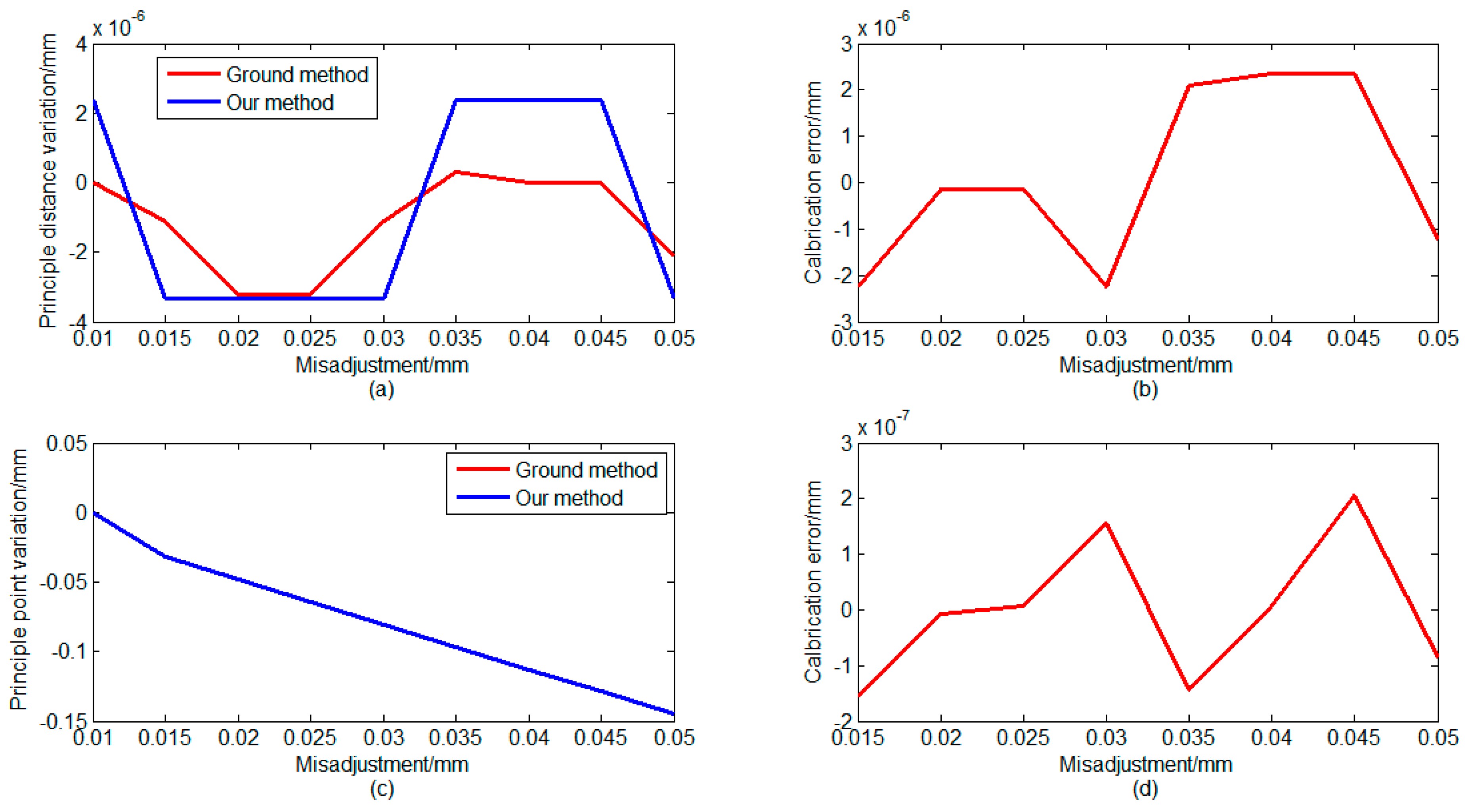
3.1. Simulation and Analysis
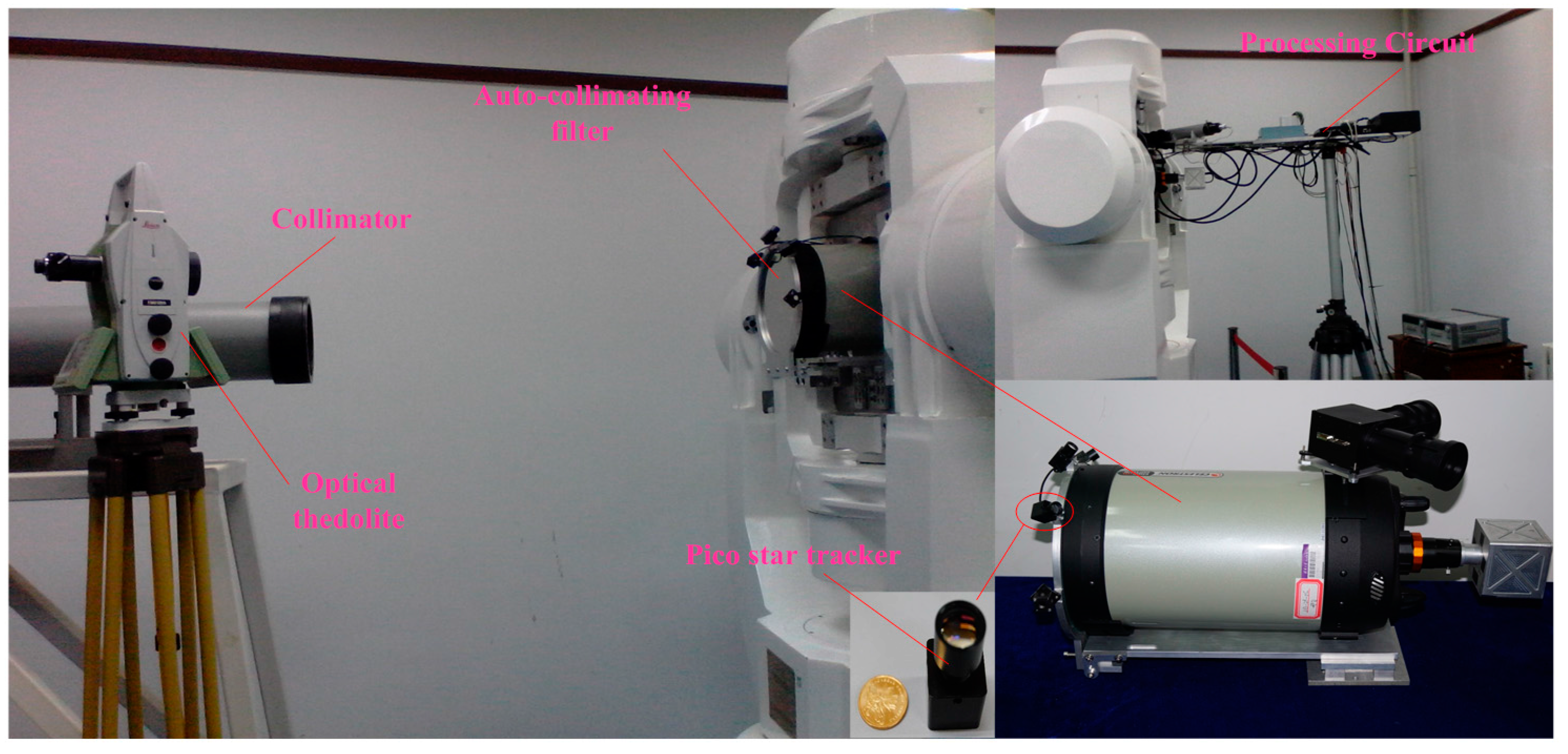
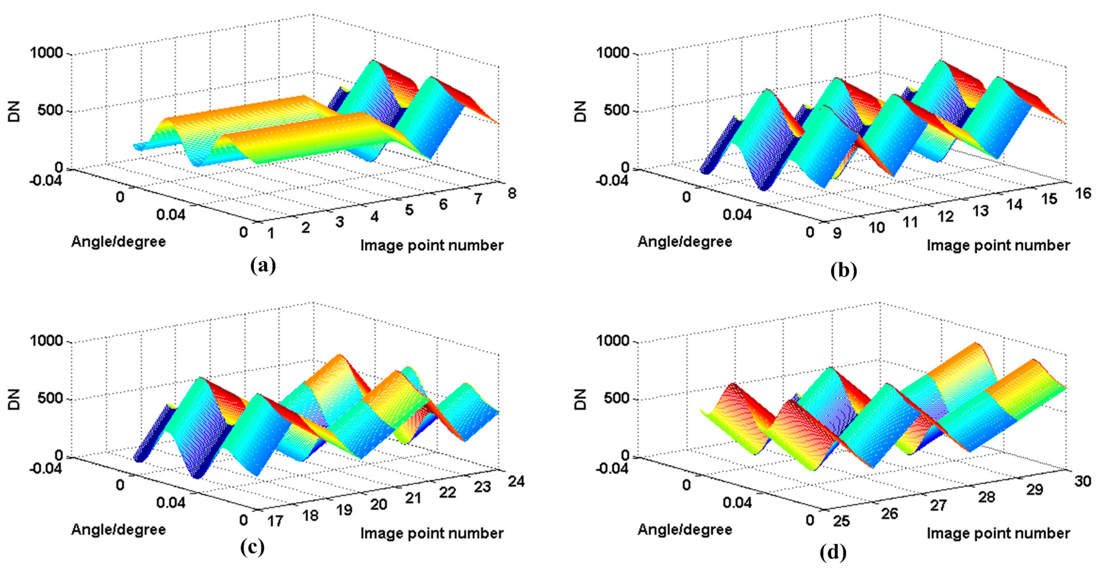
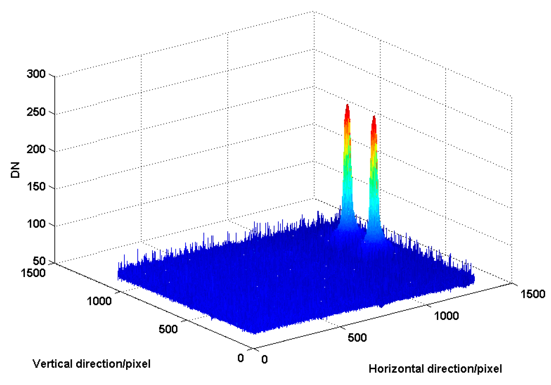
3.2. Experiments
4. Conclusions
Acknowledgments
Author Contributions
Conflicts of Interest
References
- Figoski, J.W. Quickbird telescope: The reality of large high-quality commercial space optics. Proc. SPIE 1999, 3779, 22–30. [Google Scholar]
- Han, C. Recent Earth imaging commercial satellites with high resolutions. Chin. J. Opt. Appl. Opt. 2010, 3, 202–208. [Google Scholar]
- Wei, M.; Xing, F.; You, Z. An implementation method based on ERS imaging mode for sun sensor with 1 kHz update rate and 1 precision level. Opt. Express 2013, 21, 32524–32533. [Google Scholar] [CrossRef] [PubMed]
- Sun, T.; Xing, F.; You, Z.; Wei, M.S. Motion-blurred star acquisition method of the star tracker under high dynamic con-ditions. Opt. Express 2013, 21, 20096–20110. [Google Scholar] [CrossRef] [PubMed]
- You, Z.; Wang, C.; Xing, F.; Sun, T. Key technologies of smart optical payload in space remote sensing. Spacecr. Recover. Remote Sens. 2013, 34, 35–43. [Google Scholar]
- Li, J.; Xing, F.; You, Z. Space high-accuracy intelligence payload system with integrated attitude and position determination. Instrument 2015, 2, 3–16. [Google Scholar]
- Wang, C.; You, Z.; Xing, F.; Zhang, G. Image motion velocity field for wide view remote sensing camera and detectors exposure integration control. Acta Opt. Sin. 2013, 33, 88–95. [Google Scholar] [CrossRef]
- Wang, C.; Xing, F.; Wang, H.; You, Z. Optical flow method for lightweight agile remote sensor design and instrumentation. Proc. SPIE 2013, 8908, 1–10. [Google Scholar]
- Wang, C.; You, Z.; Xing, F.; Zhao, B.; Li, B.; Zhang, G.; Tao, Q. Optical flow inversion for remote sensing image dense registration and sensor’s attitude motion high-accurate measurement. Math. Probl. Eng. 2014, 2014, 432613. [Google Scholar] [CrossRef]
- Hong, Y.; Ren, G.; Liu, E. Non-iterative method for camera calibration. Opt. Express 2007, 23, 23992–24003. [Google Scholar] [CrossRef] [PubMed]
- Ricolfe-Viala, C.; Sanchez-Salmeron, A.; Valera, A. Calibration of a trinocular system formed with wideangle lens cameras. Opt. Express 2012, 20, 27691–27696. [Google Scholar] [CrossRef] [PubMed]
- Lin, P.D.; Sung, C.K. Comparing two new camera calibration methods with traditional pinhole calibrations. Opt. Express 2007, 15, 3012–3022. [Google Scholar] [CrossRef] [PubMed]
- Wei, Z.; Liu, X. Vanishing feature constraints calibration method for binocular vision sensor. Opt. Express 2008, 23, 18897–18914. [Google Scholar] [CrossRef] [PubMed]
- Bauer, M.; Grießbach, D.; Hermerschmidt, A.; Krüger, S.; Scheele, M.; Schischmanow, A. Geometrical camera calibration with diffractive optical elements. Opt. Express 2008, 16, 20241–20248. [Google Scholar] [CrossRef] [PubMed]
- Yilmazturk, F. Full-automatic self-calibration of color digital cameras using color targets. Opt. Express 2011, 19, 18164–18174. [Google Scholar] [CrossRef] [PubMed]
- Ricolfe-Viala, C.; Sanchez-Salmeron, A. Camera calibration under optimal conditions. Opt. Express 2011, 19, 10769–10775. [Google Scholar] [CrossRef] [PubMed]
- Simon, T.; Aymen, A.; Pierre, D. Cross-diffractive optical elements for wide angle geometric camera calibration. Opt. Lett. 2011, 36, 4770–4772. [Google Scholar]
- Heikkila, J.; Silven, O. A four-step camera calibration procedure with implicit image correction. In Proceedings of the IEEE Computer Society Conference on Computer Vision and Pattern Recognition, San Juan, Puerto Rico, 17–19 June 1997; pp. 1106–1112.
- Maybank, S.J.; Faugeras, O.D. A theory of self-calibration of a moving camera. Int. J. Comput. Vis. 1992, 8, 123–151. [Google Scholar] [CrossRef]
- Faugeras, O.D.; Luong, Q.T.; Maybank, S.J. Camera self-calibration: Theory and experiments. In Computer Vision ECCV’92; Springer: Berlin/Heidelberg, Germany, 1992; pp. 321–334. [Google Scholar]
- Hartley, R.I. Euclidean reconstruction from uncalibrated views. In Applications of Invariance in Computer Vision; Springer: Berlin/Heidelberg, Germany, 1994; pp. 235–256. [Google Scholar]
- Song, D.M. A self-calibration technique for active vision system. IEEE Trans. Robot. Autom. 1996, 12, 114–120. [Google Scholar] [CrossRef]
- Caprile, B.; Torre, V. Using vanishing points for camera calibration. Int. J. Comput. Vis. 1990, 4, 127–139. [Google Scholar] [CrossRef]
- Gonzalez-Aguilera, D.; Rodriguez-Gonzalvez, P.; Armesto, J.; Arias, P. Trimble Gx200 and Riegl LMS-Z390i sensor self-calibration. Opt. Express 2011, 19, 2676–2693. [Google Scholar] [CrossRef] [PubMed]
- Fraser, C.S. Photogrammetric camera component calibration: A review of analytical techniques. In Calibration and Orientation of Cameras in Computer Vision; Gruen, A., Huang, T.S., Eds.; Springer: Berlin, Germany, 2001; pp. 95–121. [Google Scholar]
- Lichti, D.D.; Kim, C. A Comparison of Three Geometric Self-Calibration Methods for Range Cameras. Remote Sens. 2011, 3, 1014–1028. [Google Scholar] [CrossRef]
- Lipski, C.; Bose, D.; Eisemann, M.; Berger, K.; Magnor, M. Sparse bundle adjustment speedup strategies. In WSCG Short Papers Post-Conference Proceedings, Proceedings of the 18th International Conference in Central Europe on Computer Graphics, Visualization and Computer Vision in Co-Operation with EUROGRAPHICS, Plzen, Czech Republic, 1–4 February 2010; Skala, V., Ed.; WSCG: Plzen, Czech Republic, 2010. [Google Scholar]
- De Lussy, F.; Greslou, D.; Dechoz, C.; Amberg, V.; Delvit, J.M.; Lebegue, L.; Blanchet, G.; Fourest, S. Pleiades HR in flight geometrical calibration: Localisation and mapping of the focalplane. In Proceedings of the XXII ISPRS Congress International Archives of the Photogrammetry, Remote Sensing and Spatial Information Sciences, Melbourne, Australia, 25 August–1 September 2012; pp. 519–523.
- Fourest, S.; Kubik, P.; Lebegu, L.; Dechoz, C.; Lacherade, S.; Blanchet, G. Star-based methods for Pleiades HR commissioning. In Proceedings of the XXII ISPRS Congress International Archives of the Photogrammetry, Remote Sensing and Spatial Information Sciences, Melbourne, Australia, 25 August–1 September 2012; pp. 531–536.
- Greslou, D.; Lussy, F.D.; Amberg, V.; Dechoz, C.; Lenoir, F.; Delvit, J.; Lebegue, L. Pleiades-HR 1A&1B image quality commissioning: Innovative geometric calibration methods and results. Proc. SPIE 2013, 8866, 1–12. [Google Scholar]
- Delvit, J.M.; Greslou, D.; Amberg, V.; Dechoz, C.; de Lussy, F.; Lebegue, L.; Latry, C.; Artigues, S.; Bernard, L. Attitude assessment using Pléiades-HR capabilities. In Proceedings of the XXII ISPRS Congress International Archives of the Photogrammetry, Remote Sensing and Spatial Information Sciences, Melbourne, Australia, 25 August–1 September 2012; pp. 525–530.
- Cook, M.K.; Peterson, B.A.; Dial, G.; Gibson, L.; Gerlach, F.W.; Hutchins, K.S.; Kudola, R.; Bowen, H.S. IKONOS Technical performance Assessment. Proc. SPIE 2001, 4381, 94–108. [Google Scholar]
- Kaveh, D.; Mazlan, H. Very high resolution optical satellites for DEM generation: A review. Eur. J. Sci. Res. 2011, 49, 542–554. [Google Scholar]
- Jacobsen, K. Geometric calibration of space remote sensing cameras for efficient processing. Int. Arch. Photogramm. Remote Sens. 1998, 32, 33–43. [Google Scholar]
- Mi, W.; Bo, Y.; Fen, H.; Xi, Z. On-orbit geometric calibration model and its applications for high-resolution optical satellite imagery. Remote Sens. 2014, 6, 4391–4408. [Google Scholar]
- Xu, Y.; Liu, T.; You, H.; Dong, L.; Liu, F. On-orbit calibration of interior orientation for HJ1B-CCD camera. Remote Sens. Technol. Appl. 2011, 26, 309–314. [Google Scholar]
- Lv, H.; Han, C.; Xue, X.; Hu, C.; Yao, C. Autofocus method for scanning remote sensing camera. Appl. Opt. 2015, 54, 6351–6359. [Google Scholar] [CrossRef] [PubMed]
- Li, J.; Chen, X.; Tian, L.; Lian, F. Tracking radiometric responsivity of optical sensors without on-board calibration systems-case of the Chinese HJ-1A/1B CCD sensors. Opt. Express 2015, 23, 1829–1847. [Google Scholar] [CrossRef] [PubMed]
- Li, J.; Xing, F.; Sun, T.; You, Z. Efficient assessment method of on-board modulation transfer function of optical remote sensing sensors. Opt. Express 2015, 23, 6187–6208. [Google Scholar] [CrossRef] [PubMed]
- Gleyzes, M.A.; Perret, L.; Kubik, P. Pleiades system architecture and main performances. In Proceedings of the XXII ISPRS Congress International Archives of the Photogrammetry, Remote Sensing and Spatial Information Sciences, Melbourne, Australia, 25 August–1 September 2012; pp. 537–542.
- Poli, D.; Remondino, F.; Angiuli, E.; Agugiaro, G. Radiometric and geometric evaluation of GeoEye-1, WorldView-2 and Pleiades stereo images for 3D information extraction. ISPRS J. Photogramm. Remote Sens. 2015, 100, 35–47. [Google Scholar] [CrossRef]
- Fu, R.; Zhang, Y.; Zhang, J. Study on geometric measurement methods for line-array stereo mapping camera. Spacecr. Recover. Remote Sens. 2011, 32, 62–67. [Google Scholar]
- Hieronymus, J. Comparaision of methods for geometric camera calibration. In Proceedings of the XXII ISPRS Congress International Archives of the Photogrammetry, Remote Sensing and Spatial Information Sciences, Melbourne, Australia, 25 August–1 September 2012; pp. 595–599.
- Yuan, F.; Qi, W.J.; Fang, A.P. Laboratory geometric calibration of areal digital aerial camera. IOP Conf. Ser. Earth Enviton. Sci. 2014, 17, 012196. [Google Scholar] [CrossRef]
- Chen, T.; Shibasaki, R.; Lin, Z. A rigorous laboratory calibration method for interior orientation of airborne linear push-broom camera. Photogramm. Eng. Remote Sens. 2007, 73, 369–374. [Google Scholar] [CrossRef]
- Wu, G.; Han, B.; He, X. Calibration of geometric parameters of line array CCD camera based on exact measuring angle in lab. Opt. Precis. Eng. 2007, 15, 1628–1632. [Google Scholar]
- Yuan, F.; Qi, W.; Fang, A.; Ding, P.; Yu, X. Laboratory geometric calibration of non-metric digital camera. Proc. SPIE 2013, 8921, 99–103. [Google Scholar]


| Elements | Ground Method | Our Method | Misadjustment (mm) |
|---|---|---|---|
| f (mm) | 2031.999999 | 2032.000 | 0 |
| Δf (mm) | 8.527259 × 10⁻⁷ | 0 | 0 |
| U0x (mm) | 0 | 0 | 0 |
| U0y (mm) | 0 | 0 | 0 |
| ΔU0x (mm) | 0 | 0 | 0 |
| ΔU0y (mm) | 0 | 0 | 0 |
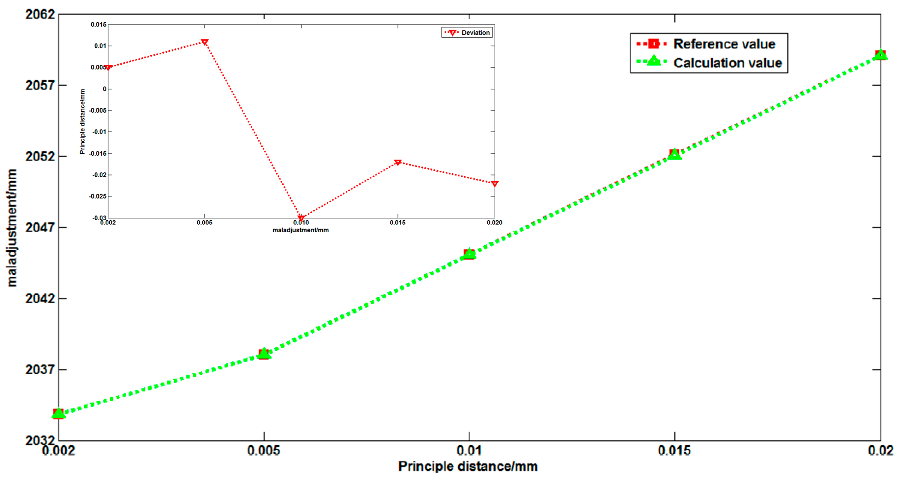
| Number | Elements | Reference Value |
|---|---|---|
| 1 | f (mm) | 2032.1161 |
| 2 | U0x (mm) | –0.5856 |
| 3 | U0y (mm) | –0.9643 |
| Number | Elements | Calibration Value |
|---|---|---|
| 1 | f (mm) | 2032.0818 |
| 2 | U0x (mm) | –0.5387 |
| 3 | U0y (mm) | –0.9580 |
| 4 | Δf (mm) | 0.0342 |
| 5 | ΔU0x (mm) | 0.0469 |
| 6 | ΔU0y (mm) | 0.0063 |
© 2016 by the authors; licensee MDPI, Basel, Switzerland. This article is an open access article distributed under the terms and conditions of the Creative Commons Attribution (CC-BY) license (http://creativecommons.org/licenses/by/4.0/).
Share and Cite
Li, J.; Xing, F.; Chu, D.; Liu, Z. High-Accuracy Self-Calibration for Smart, Optical Orbiting Payloads Integrated with Attitude and Position Determination. Sensors 2016, 16, 1176. https://doi.org/10.3390/s16081176
Li J, Xing F, Chu D, Liu Z. High-Accuracy Self-Calibration for Smart, Optical Orbiting Payloads Integrated with Attitude and Position Determination. Sensors. 2016; 16(8):1176. https://doi.org/10.3390/s16081176
Chicago/Turabian StyleLi, Jin, Fei Xing, Daping Chu, and Zilong Liu. 2016. "High-Accuracy Self-Calibration for Smart, Optical Orbiting Payloads Integrated with Attitude and Position Determination" Sensors 16, no. 8: 1176. https://doi.org/10.3390/s16081176