
On Connectivity of Wireless Sensor Networks with Directional Antennas


Abstract
:1. Introduction
- We establish a general framework to analyze the network connectivity with various existing directional antenna models and our proposed iris model. In particular, we investigate both the local connectivity and the overall connectivity of WSNs in the presence of channel randomness. More specifically, the local connectivity mainly concerns the probability of the node isolation of a node, while the overall connectivity evaluates the probability that there exists at least one path for each node pair in the network from the viewpoint of the entire network.
- We conduct extensive simulations to validate the analytical framework and evaluate the accuracy of the existing antenna models and our proposed model. Our simulation results match the analytical results, indicating that the analytical framework is quite accurate and effective. Besides, our proposed iris model provides a relatively better approximation to realistic antennas than the keyhole model and the sector model on average.
- We find that the network connectivity heavily depends on different antenna models and different channel conditions. We demonstrate that the channel randomness (such as the path loss and the shadow fading) has significant impacts on the network connectivity. For example, the path loss effect is always detrimental to the network connectivity, and the shadow fading effect is somewhat beneficial to the connectivity.
2. Related Works
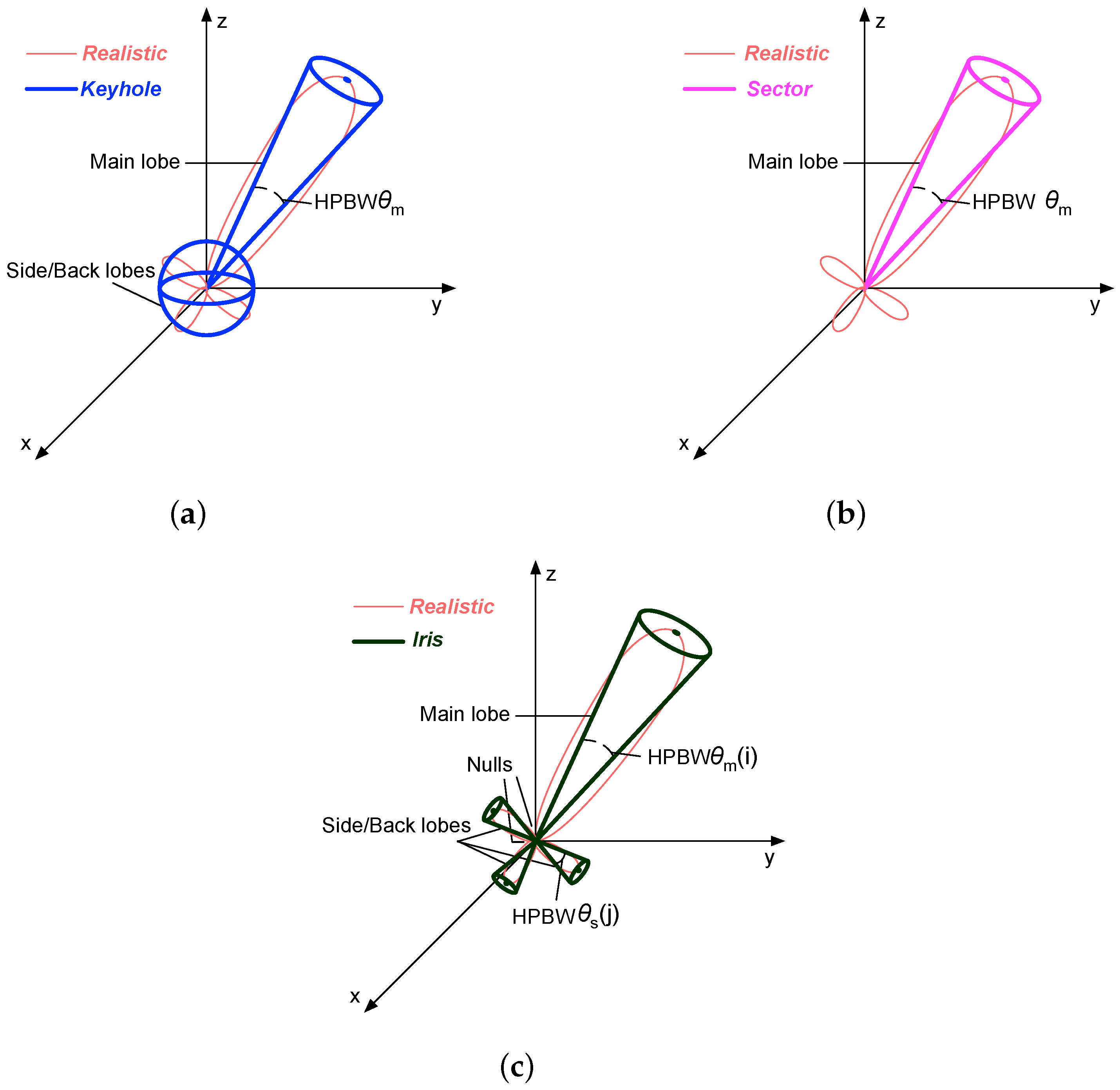
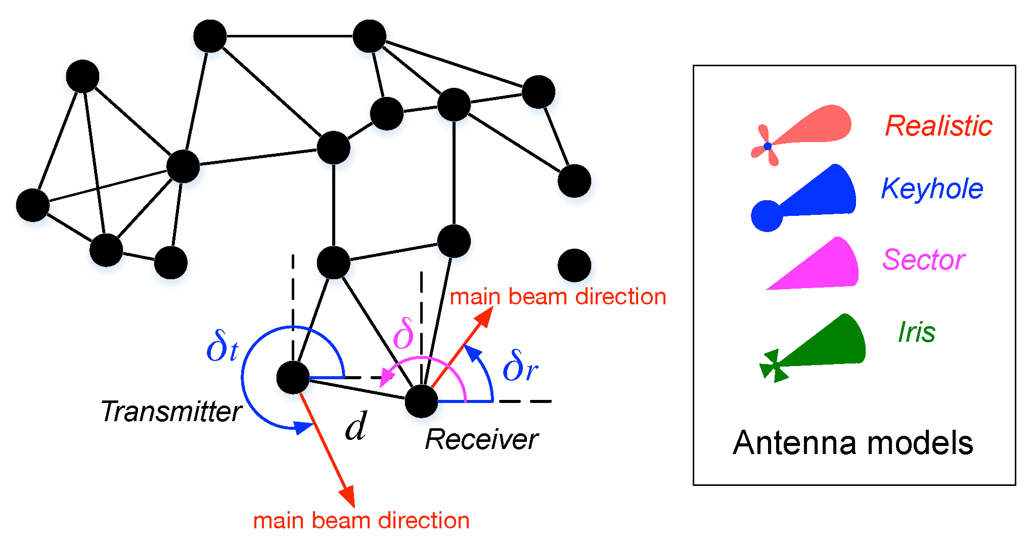
3. Antenna Models
3.1. Isotropic Antenna
3.2. Directional Antennas
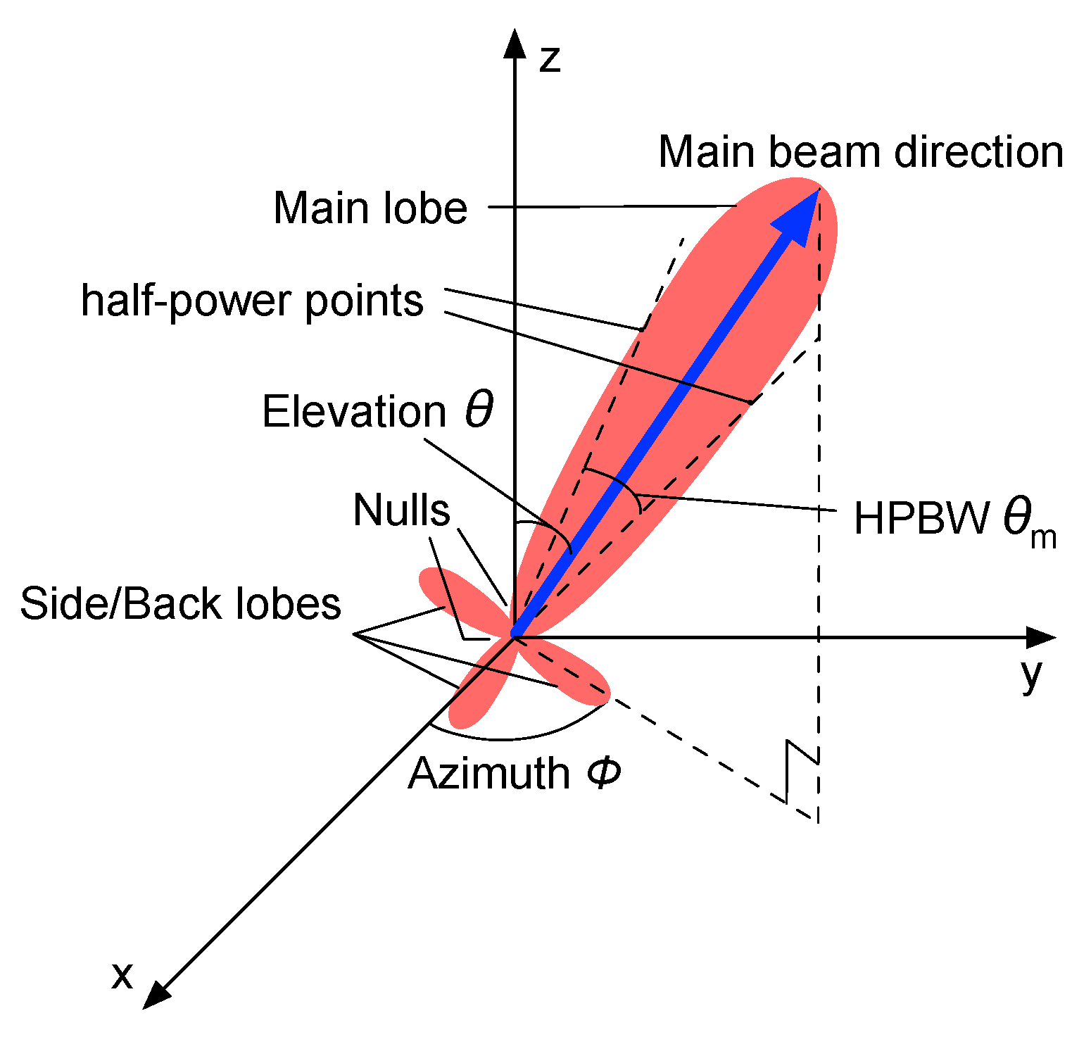
- The radiation beam (lobe) is a clear peak in the radiation intensity surrounded by regions of weaker radiation intensity.
- The Half Power Beam Width (HPBW) is the angular width between the half-power (−3 dB) points of the lobe.
- The main beam represents the radiation lobe with the maximum antenna gain.
- The side or back lobes represent the lobes in any directions other than the direction of the main beam.
- The nulling capability is the capability of a directional antenna employing nulls to counteract unwanted interference in some undesired directions.
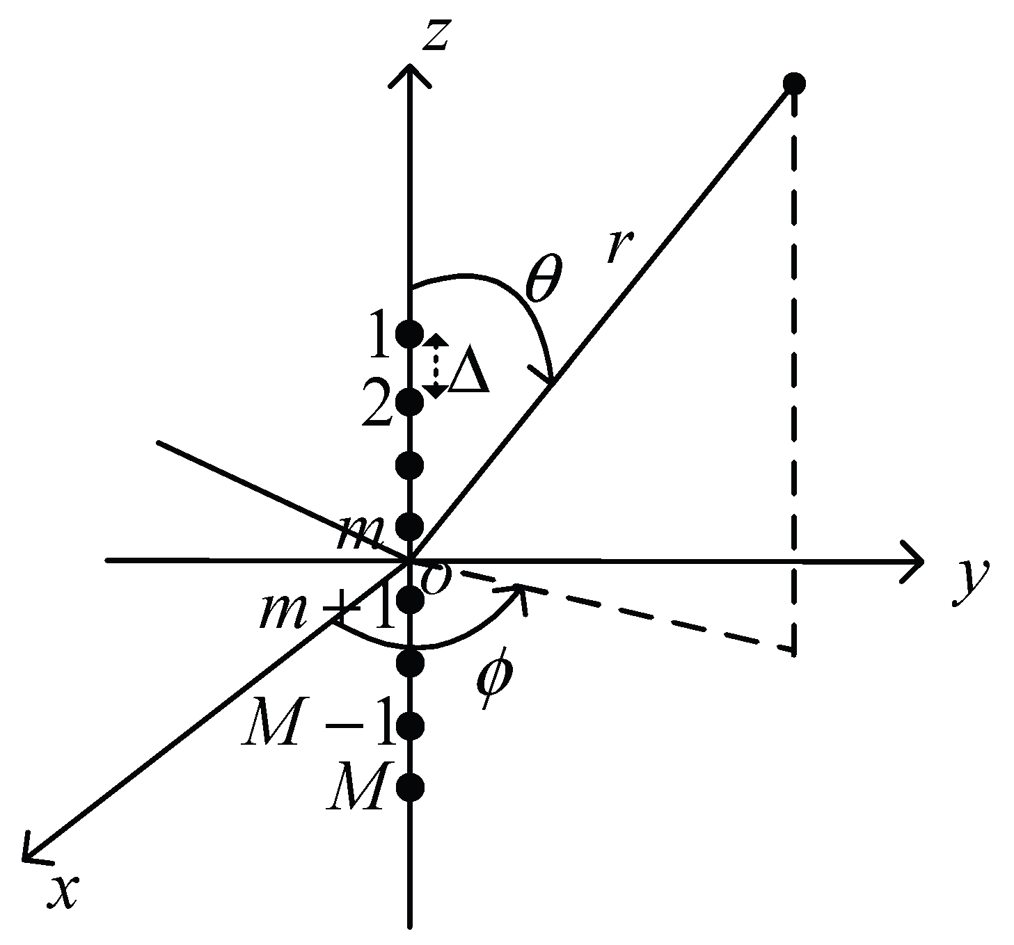
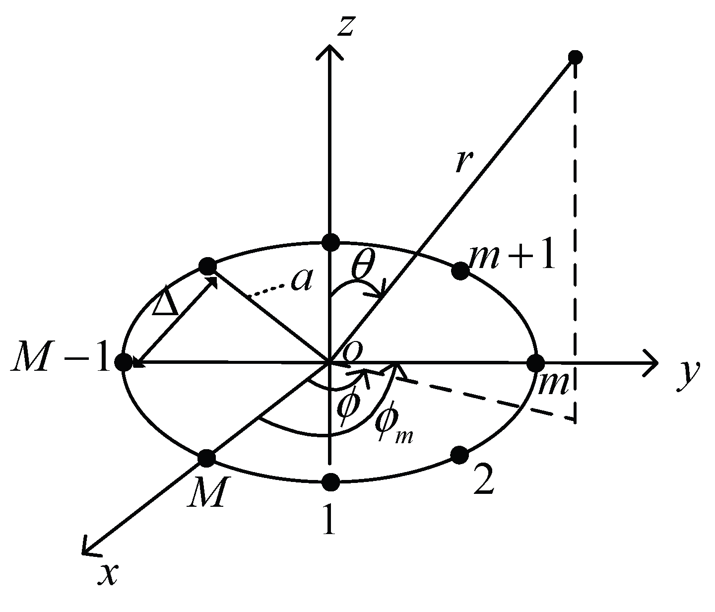
3.2.1. Uniform Circular Array
3.2.2. Uniform Linear Array
3.3. Existing Simplified Models of Directional Antennas
3.4. Iris Antenna Model
4. Channel Models
5. Local Connectivity
5.1. Probability of Isolation
5.2. Empirical Results of Local Connectivity
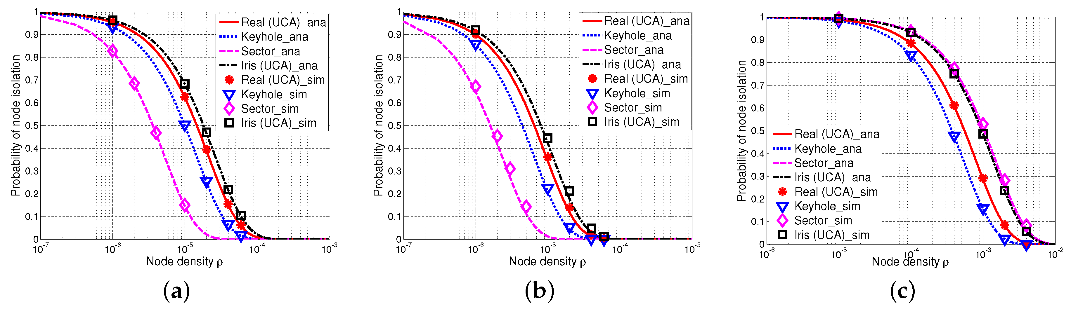
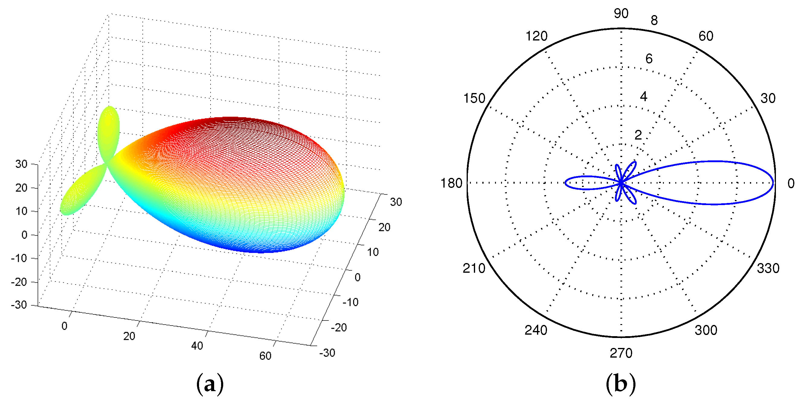
5.2.1. Comparisons of the Probability of Node Isolation with UCA Antennas, Keyhole, Sector and Iris-UCA Models
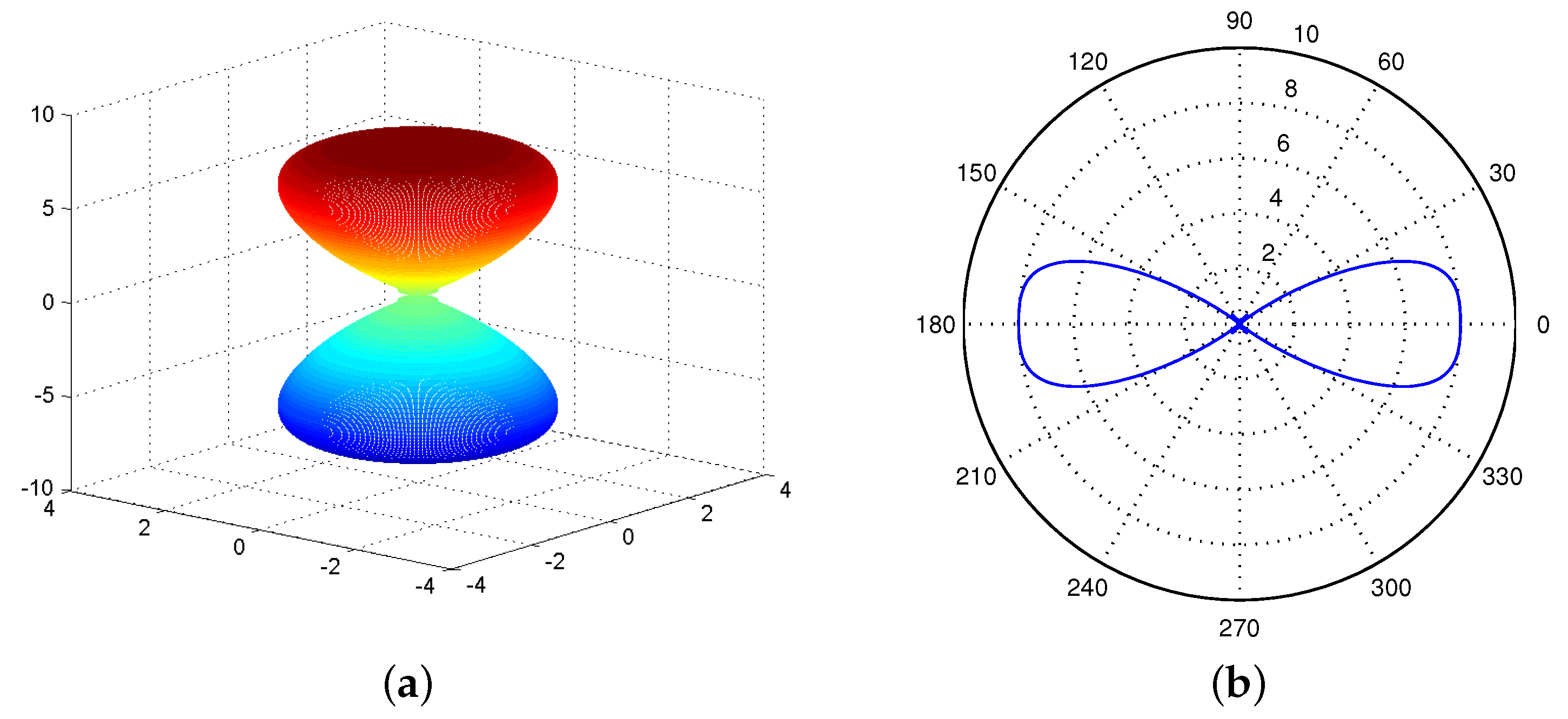
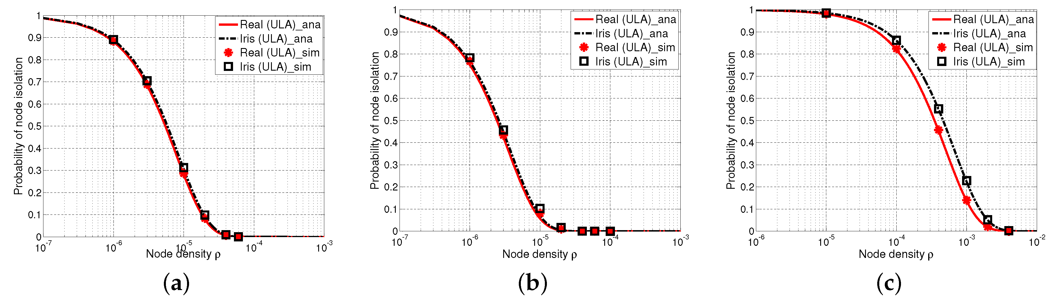
5.2.2. Comparisons of the Probability of Node Isolation with the ULA Antenna and Iris-ULA Model
6. Overall Connectivity
6.1. One-Connectivity
6.2. Empirical Results of One-Connectivity
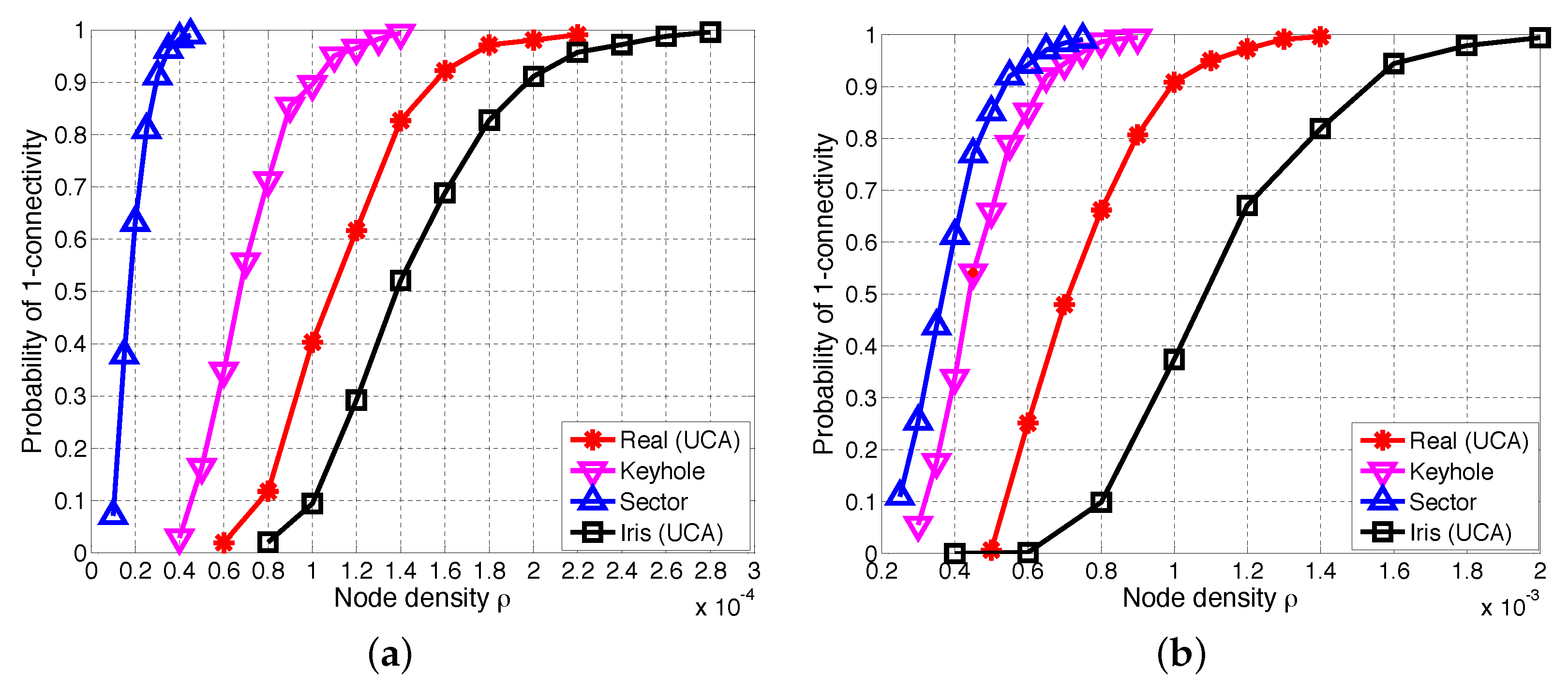
6.2.1. Comparisons of One-Connectivity with UCA Antenna, Keyhole, Sector and Iris-UCA Models
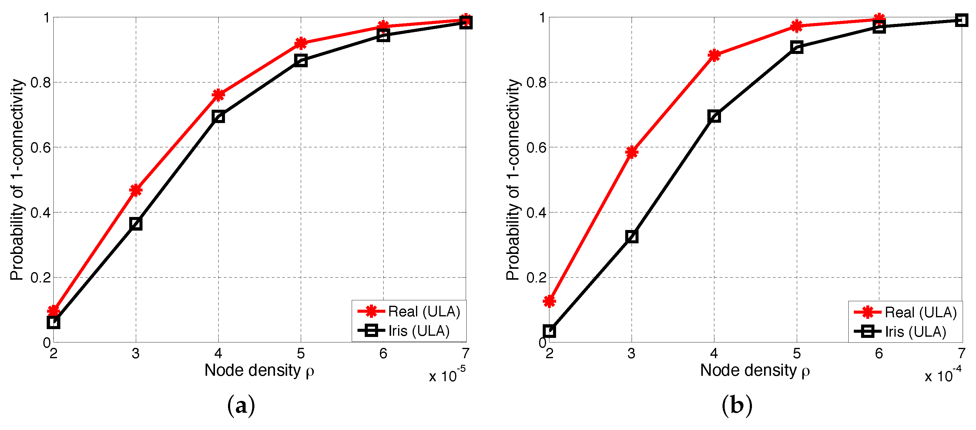
6.2.2. Comparisons of One-Connectivity with ULA Antenna and Iris-ULA Model
7. Discussion and Future Directions
8. Conclusions
Acknowledgments
Author Contributions
Conflicts of Interest
References
- Dousse, O.; Baccelli, F.; Thiran, P. Impact of interferences on connectivity in ad-hoc networks. IEEE/ACM Trans. Netw. Inf. 2005, 13, 425–436. [Google Scholar] [CrossRef]
- Bettstetter, C. On the Connectivity of Ad Hoc Networks. Comput. J. 2004, 47, 432–447. [Google Scholar] [CrossRef]
- Zhang, J.; Jia, X. Capacity analysis of wireless mesh networks with omni or directional antennas. In Proceedings of the IEEE INFOCOM (Mini-Conference), Rio de Janeiro, Brazil, 19–25 April 2009.
- Dai, H.N.; Ng, K.W.; Wong, R.C.W.; Wu, M.Y. On the Capacity of Multi-Channel Wireless Networks Using Directional Antennas. In Proceedings of the 27th Conference on Computer Communications INFOCOM 2008, Phoenix, AZ, USA, 13–18 April 2008.
- Dai, H.N. Throughput and Delay in Wireless Sensor Networks using Directional Antennas. In Proceedings of the Fifth International Conference on Intelligent Sensors, Sensor Networks and Information Processing (ISSNIP), Melbourne, Australia, 7–10 December 2009.
- Min, B.C.; Matson, E.T.; Khaday, B. Design of a Networked Robotic System Capable of Enhancing Wireless Communication Capabilities. In Proceedings of the 2013 IEEE International Symposium on Safety, Security, and Rescue Robotics (SSRR), Linköping, Sweden, 21–26 October 2013; pp. 1–8.
- Georgiou, O.; Wang, S.; Bocus, M.Z.; Dettmann, C.P.; Coon, J.P. Directional antennas improve the link-connectivity of interference limited ad hoc networks. In Proceedings of the 26th Annual International Symposium on Personal, Indoor, and Mobile Radio Communications (PIMRC), Hong Kong, China, 30 August–2 September 2015; pp. 1311–1316.
- Min, B.C.; Matson, E.T.; Jung, J.W. Active Antenna Tracking System with Directional Antennas for Enhancing Wireless Communication Capabilities of a Networked Robotic System. J. Field Robot. 2015. [Google Scholar] [CrossRef]
- Rangan, S.; Rappaport, T.S.; Erkip, E. Millimeter Wave Cellular Wireless Networks: Potentials and Challenges. Proc. IEEE 2014, 102, 366–385. [Google Scholar] [CrossRef]
- Qiao, J.; Shen, X.; Mark, J.W.; Shen, Q.; He, Y.; Lei, L. Enabling Device-to-Device Communications in Millimeter-Wave 5G Cellular Networks. IEEE Commun. Mag. 2015, 53, 209–215. [Google Scholar] [CrossRef]
- Bai, T.; Robert, W.; Heath, J. Coverage and Rate Analysis for Millimeter Wave Cellular Networks. IEEE Trans. Wirel. Commun. 2014, 14, 1100–1114. [Google Scholar] [CrossRef]
- Thornburg, A.; Bai, T.; Robert, W.; Heath, J. Performance Analysis of Outdoor mmWave Ad Hoc Networks. IEEE Trans. Signal Process. 2016, 64, 4065–4079. [Google Scholar] [CrossRef]
- Sulyman, A.I.; Alwarafy, A.; MacCartney, G.R.; Rappaport, T.S.; Alsanie, A. Directional Radio Propagation Path Loss Models for Millimeter-Wave Wireless Networks in the 28-, 60-, and 73-GHz Bands. IEEE Trans. Wirel. Commun. 2016, 15, 6939–6947. [Google Scholar] [CrossRef]
- Nitsche, T.; Cordeiro, C.; Flores, A.; Knightly, E.W.; Perahia, E.; Widmer, J.C. IEEE 802.11ad: Directional 60 GHz communication for multi-Gigabit-per-second Wi-Fi. IEEE Commun. Mag. 2014, 52, 132–141. [Google Scholar] [CrossRef]
- Saha, S.K.; Vira, V.V.; Garg, A.; Koutsonikolas, D. Multi-Gigabit indoor WLANs: Looking beyond 2.4/5 GHz. In Proceedings of the IEEE International Conference on Communications (ICC), Kuala Lumpur, Malaysia, 22–27 May 2016.
- Min, B.C.; Lewis, J.; Matson, E.T.; Smith, A.H. Heuristic optimization techniques for self-orientation of directional antennas in long-distance point-to-point broadband networks. J. Ad Hoc Netw. 2013, 11, 2252–2263. [Google Scholar] [CrossRef]
- Min, B.C.; Matson, E.T. Robotic Follower System Using Bearing-Only Tracking with Directional Antennas. In Robot Intelligence Technology and Applications 2; Springer: Basel, Switzerland, 2014; pp. 37–58. [Google Scholar]
- Ramanathan, R.; Redi, J.; Santivanez, C.; Wiggins, D.; Polit, S. Ad Hoc Networking With Directional Antennas: A Complete System Solution. IEEE JSAC 2005, 23, 496–506. [Google Scholar] [CrossRef]
- Zhou, X.; Durrani, S.; Jones, H. Connectivity Analysis of Wireless Ad Hoc Networks with Beamforming. IEEE Trans. Veh. Technol. 2009, 58, 5247–5257. [Google Scholar] [CrossRef]
- Kiese, M.; Hartmann, C.; Vilzmann, R. Optimality Bounds of the Connectivity of Adhoc Networks with Beamforming Antennas. In Proceedings of the IEEE GLOBECOM 2009—2009 IEEE Global Telecommunications Conference, Honolulu, HI, USA, 30 November–4 December 2009.
- Chau, C.K.; Gibbens, R.J.; Towsley, D. Impact of directional transmission in large-scale multi-hop wireless ad hoc networks. In Proceedings of the 2012 IEEE INFOCOM, Orlando, FL, USA, 25–30 March 2012; pp. 522–530.
- Dai, H.N.; Ng, K.W.; Wu, M.Y. On Busy-Tone Based MAC Protocol for Wireless Networks with Directional Antennas. Wirel. Pers. Commun. 2013, 73, 611–636. [Google Scholar] [CrossRef]
- Park, L.; Lee, C.G.; Cho, S. SPARM: Spatially Pipelined ACK Aggregation for Reliable Multicast in Directional MAC. IEEE Commun. Lett. 2013, 17, 596–599. [Google Scholar] [CrossRef]
- Yuan, X.; Li, C.; Song, Y.; Yang, L.; Ullah, S. On Energy-Saving in E-Healthcare: A Directional MAC Protocol for WBAN. In Proceedings of the 2015 IEEE Globecom Workshops (GC Wkshps), San Diego, CA, USA, 6–10 December 2015; pp. 1–6.
- Wang, P.; Petrova, M. Cross Talk MAC: A Directional MAC Scheme for Enhancing Frame Aggregation in mm-Wave Wireless Personal Area Networks. In Proceedings of the 2016 IEEE International Conference on Communications Workshops (ICC), Kuala Lumpur, Malaysia, 23–27 May 2016; pp. 602–607.
- Dai, H.N.; Zhao, Q. On the delay reduction of wireless ad hoc networks with directional antennas. EURASIP J. Wirel. Commun. Network. 2015, 2015, 1–13. [Google Scholar] [CrossRef]
- Renzo, M.D. Stochastic Geometry Modeling and Performance Evaluation of mmWave Cellular Communications. In Proceedings of the 2015 IEEE International Conference on Communications (ICC), London, UK, 8–12 June 2015; pp. 5992–5997.
- Li, P.; Zhang, C.; Fang, Y. The Capacity of Wireless Ad Hoc Networks Using Directional Antennas. IEEE Trans. Mob. Comput. 2011, 10, 1374–1387. [Google Scholar] [CrossRef]
- Gupta, P.; Kumar, P.R. Critical power for asymptotic connectivity in wireless networks. In Stochastic Analysis, Control, Optimization and Applications: A Volume in Honor of W. H. Fleming; Birkhäuser: Boston, MA, USA, 1998; pp. 547–566. [Google Scholar]
- Bettstetter, C.; Hartmann, C. Connectivity of Wireless Multihop Networks in a Shadow Fading Environment. ACM Wirel. Netw. 2005, 11, 571–589. [Google Scholar] [CrossRef]
- Miorandi, D.; Altman, E.; Alfano, G. The Impact of Channel Randomness on Coverage and Connectivity of Ad Hoc and Sensor Networks. IEEE Trans. Wirel. Commun. 2008, 7, 1062–1072. [Google Scholar] [CrossRef]
- Zhu, C.; Zheng, C.; Shu, L.; Han, G. A survey on coverage and connectivity issues in wireless sensor networks. J. Netw. Comput. Appl. 2012, 35, 619–632. [Google Scholar] [CrossRef]
- Zhai, D.; Sheng, M.; Wang, X.; Zhang, Y. Local Connectivity of Cognitive Radio Ad Hoc Networks. In Proceedings of the IEEE Global Communications Conference (GLOBECOM), Austin, TX, USA, 8–12 December 2014.
- Dai, H.N.; Ng, K.W.; Li, M.; Wu, M.Y. An Overview of Using Directional Antennas in Wireless Networks. Int. J. Commun. Syst. 2013, 26, 413–448. [Google Scholar] [CrossRef]
- Dai, H.N.; Wang, Q.; Li, D.; Wong, R.C.W. On Eavesdropping Attacks in Wireless Sensor Networks with Directional Antennas. Int. J. Distrib. Sens. Netw. 2013, 2013. [Google Scholar] [CrossRef]
- Li, X.; Xu, J.; Dai, H.N.; Zhao, Q.; Cheang, C.F.; Wang, Q. On Modeling Eavesdropping Attacks in Wireless Networks. J. Comput. Sci. 2015, 11, 196–204. [Google Scholar] [CrossRef]
- Basikolo, T.; Arai, H. APRD-MUSIC Algorithm DOA Estimation for Reactance Based Uniform Circular Array. IEEE Trans. Antennas Propag. 2016, 64, 4415–4422. [Google Scholar] [CrossRef]
- Bettstetter, C.; Hartmann, C.; Moser, C. How does randomized beamforming improve the connectivity of ad hoc networks. In Proceedings of the 2005 IEEE International Conference on Communications, Seoul, Korea, 16–20 May 2005.
- Zhou, X.; Jones, H.M.; Durrani, S.; Scott, A. Effect of Beamforming on the Connectivity of Ad Hoc Networks. In Proceedings of the Australian Communications Theory Workshop (AusCTW), Adelaide, Australia, 5–7 February 2007.
- Li, P.; Zhang, C.; Fang, Y. Asymptotic Connectivity in Wireless Ad Hoc Networks Using Directional Antenna. IEEE/ACM Trans. Netw. 2009, 17, 1106–1117. [Google Scholar]
- Xu, H.; Dai, H.N.; Zhao, Q. On the Connectivity of Wireless Networks with Multiple Directional Antennas. In Proceedings of the 18th IEEE International Conference on Networks (ICON), Singapore, 12–14 December 2012.
- Wang, P.; Li, Y.; Vucetic, B. Millimeter Wave Communications With Symmetric Uniform Circular Antenna Arrays. IEEE Commun. Lett. 2014, 18, 1307–1310. [Google Scholar] [CrossRef]
- Wang, Q.; Dai, H.N.; Zhao, Q. Connectivity of Wireless Ad Hoc Networks: Impacts of Antenna Models. In Proceedings of the 14th International Conference on Parallel and Distributed Computing, Applications and Technologies, Taipei, Taiwan, 16–18 December 2013.
- Balanis, C.A. Antenna Theory: Analysis and Design, 3rd ed.; John Wiley & Sons: New York, NY, USA, 2005. [Google Scholar]
- Jackson, B.R.; Rajan, S.; Liao, B.J.; Wang, S. Direction of Arrival Estimation Using Directive Antennas in Uniform Circular Arrays. IEEE Trans. Antennas Propag. 2015, 63, 736–747. [Google Scholar] [CrossRef]
- Gao, X.; Edfors, O.; Rusek, F.; Tufvesson, F. Massive MIMO Performance Evaluation Based on Measured Propagation Data. IEEE Trans. Wirel. Commun. 2015, 14, 3899–3911. [Google Scholar] [CrossRef]
- Cai, W.; Wang, P.; Li, Y.; Zhang, Y.; Vucetic, B. Deployment Optimization of Uniform Linear Antenna Arrays for a Two-Path Millimeter Wave Communication System. IEEE Commun. Lett. 2015, 19, 669–672. [Google Scholar] [CrossRef]
- Goldsmith, A. Wireless Communication; Cambridge University Press: Cambridge, UK, 2005. [Google Scholar]
- Rappaport, T.S. Wireless Communications: Principles and Practice, 2nd ed.; Prentice Hall PTR: Upper Saddle River, NJ, USA, 2002. [Google Scholar]
- Wackerly, D.D.; Mendenhall, W.; Scheaffer, R.L. Mathematical Statistics With Applications; Cengage Learning: Boston, MA, USA, 2007. [Google Scholar]
- Gravina, R.; Alinia, P.; Ghasemzadeh, H.; Fortino, G. Multi-Sensor Fusion in Body Sensor Networks: State-of-the-art and research challenges. Inf. Fusion 2016, 35, 68–80. [Google Scholar] [CrossRef]
- Fortino, G.; Giannantonio, R.; Gravina, R.; Kuryloski, P.; Jafari, R. Enabling Effective Programming and Flexible Management of Efficient Body Sensor Network Applications. IEEE Trans. Hum.-Mach. Syst. 2013, 43, 115–133. [Google Scholar] [CrossRef]
- Smart, G.; Deligiannis, N.; Surace, R.; Loscri, V.; Fortino, G.; Andreopoulos, Y. Decentralized Time-Synchronized Channel Swapping for Ad Hoc Wireless Networks. IEEE Trans. Veh. Technol. 2016, 65, 8538–8553. [Google Scholar] [CrossRef]
- Fortino, G.; Galzarano, S.; Gravina, R.; Li, W. A framework for collaborative computing and multi-sensor data fusion in body sensor networks. Inf. Fusion 2014, 22, 50–70. [Google Scholar] [CrossRef]
- Dong, J.; Smith, D. Joint relay selection and transmit power control for wireless body area networks coexistence. In Proceedings of the 2014 IEEE International Conference on Communications (ICC), Sydney, Australia, 10–14 June 2014; pp. 5676–5681.
- Ding, J.; Dutkiewicz, E.; Huang, X.; Fang, G. Energy-Efficient Distributed Beamforming in UWB Based Implant Body Area Networks. In Proceedings of the 2015 IEEE 81st Vehicular Technology Conference (VTC Spring), Glasgow, UK, 11–14 May 2015; pp. 1–5.


| Features | Keyhole Model | Sector Model | Iris Model (This Paper) |
|---|---|---|---|
| Main beam | Yes | Yes | Yes |
| Side/back lobes | Yes | No | Yes |
| Nulling capability | No | Yes | Yes |
| More than one main beam | No | No | Yes |
| Path Loss α | Antenna Models | |||
|---|---|---|---|---|
| UCA | Keyhole | Sector | Iris-UCA | |
| 2 | 1.61 | 2.33 (+44.34%) | 22.60 (+1302.28%) | 1.55 (−3.67%) |
| 2.25 | 1.32 | 1.92 (+45.31%) | 9.42 (+612.86%) | 1.16 (−12.28%) |
| 2.5 | 1.15 | 1.68 (+46.59%) | 4.68 (+307.40%) | 0.93 (−19.15%) |
| 2.75 | 1.04 | 1.53 (+47.72%) | 2.64 (+154.39%) | 0.78 (−24.74%) |
| 3 | 0.96 | 1.43 (+48.55%) | 1.64 (+70.14%) | 0.68 (−29.39%) |
| 3.25 | 0.91 | 1.36 (+49.06%) | 1.09 (+20.16%) | 0.61 (−33.31%) |
| 3.5 | 0.87 | 1.30 (+49.28%) | 0.77 (−11.33%) | 0.55 (−36.67%) |
| 3.75 | 0.84 | 1.26 (+49.23%) | 0.57 (−32.18%) | 0.51 (−39.56%) |
| 4 | 0.82 | 1.23 (+48.98%) | 0.44 (−46.54%) | 0.48 (−42.08%) |
| Mean absolute deviation | N/A | 47.67% | 284.14% | 26.76% |
| Path Loss α | Antenna Models | |
|---|---|---|
| Realistic ULA | Iris-ULA | |
| 2 | 6.07 | 6.26 (+3.23%) |
| 2.25 | 4.13 | 4.04 (−2.10%) |
| 2.5 | 3.08 | 2.87 (−6.64%) |
| 2.75 | 2.44 | 2.19 (−10.58%) |
| 3 | 2.04 | 1.75 (−14.04%) |
| 3.25 | 1.76 | 1.46 (−17.12%) |
| 3.5 | 1.56 | 1.25 (−19.87%) |
| 3.75 | 1.42 | 1.10 (−22.36%) |
| 4 | 1.31 | 0.99 (−24.61%) |
| Mean absolute deviation | N/A | 13.39% |
| Parameters | Values |
|---|---|
| Number of topologies | 5000 |
| Attenuation threshold | 50 dB |
| Path loss exponent α | 2.5, 4 |
| Standard deviation of shadow effect σ | 4, 8 |
| α | A (m2) | Antenna Models | |||
|---|---|---|---|---|---|
| Realistic UCA | Keyhole | Sector | Iris-UCA | ||
| 2 | 106 | 8.75 × 10⁻⁶ | 5.67 × 10⁻⁶ (−35.20%) | 3.18 × 10⁻⁷ (−96.37%) | 9.14 × 10⁻⁶ (+4.46%) |
| 2.5 | 106 | 2.10 × 10⁻⁴ | 1.37 × 10⁻⁴ (−34.76%) | 4.34 × 10⁻⁵ (−79.33%) | 2.66 × 10⁻⁴ (+26.67%) |
| 3 | 2.5 × 10⁵ | 1.32 × 10⁻³ | 8.58 × 10⁻⁴ (−35.00%) | 7.38 × 10⁻⁴ (−44.09%) | 1.90 × 10⁻³ (+43.94%) |
| 3.5 | 2.5 × 10⁵ | 5.20 × 10⁻³ | 3.35 × 10⁻³ (−35.50%) | 5.93 × 10⁻³ (+14.04%) | 8.56 × 10⁻⁴ (+64.57%) |
| 4 | 2.5 × 10⁵ | 1.40 × 10⁻² | 9.10 × 10⁻³ (−35.15%) | 2.76 × 10⁻² (+97.01%) | 2.54 × 10⁻² (+80.67%) |
| α | A (m2) | Antenna Models | |||
|---|---|---|---|---|---|
| Realistic UCA | Keyhole | Sector | Iris-UCA | ||
| 2 | 106 | 1.90 × 10⁻⁶ | 1.20 × 10⁻⁵ (−36.84%) | 2.48 × 10⁻⁸ (−98.69%) | 1.99 × 10⁻⁶ (+4.74%) |
| 2.5 | 106 | 8.46 × 10⁻⁵ | 5.50 × 10⁻⁵ (−34.99%) | 1.71 × 10⁻⁵ (−79.79%) | 1.07 × 10⁻⁴ (+26.48%) |
| 3 | 2.5 × 10⁵ | 7.06 × 10⁻⁴ | 4.57 × 10⁻⁴ (−35.27%) | 3.92 × 10⁻⁴ (−44.48%) | 1.00 × 10⁻³ (+41.64%) |
| 3.5 | 2.5 × 10⁵ | 3.30 × 10⁻³ | 2.12 × 10⁻³ (−35.61%) | 3.77 × 10⁻³ (+14.10%) | 5.44 × 10⁻³ (+64.86%) |
| 4 | 2.5 × 10⁵ | 9.93 × 10⁻³ | 6.43 × 10⁻³ (−35.22%) | 1.96 × 10⁻² (+97.31%) | 1.80 × 10⁻² (+81.23%) |
| α | A (m2) | Antenna Models | |
|---|---|---|---|
| Realistic ULA | Iris-ULA Model | ||
| 2 | 106 | 1.78 × 10⁻⁶ | 1.71 × 10⁻⁶ (−3.86%) |
| 2.5 | 106 | 6.98 × 10⁻⁵ | 7.54 × 10⁻⁵ (+8.05%) |
| 3 | 2.5 × 10⁵ | 5.75 × 10⁻⁴ | 6.81 × 10⁻⁴ (+18.39%) |
| 3.5 | 2.5 × 10⁵ | 2.74 × 10⁻³ | 3.50 × 10⁻³ (+27.53%) |
| 4 | 2.5 × 10⁵ | 8.48 × 10⁻³ | 1.15 × 10⁻³ (+35.97%) |
| α | A (m2) | Antenna Models | |
|---|---|---|---|
| Realistic ULA | Iris-ULA | ||
| 2 | 106 | 3.38 × 10⁻⁶ | 3.23 × 10⁻⁶ (−4.44%) |
| 2.5 | 106 | 2.77 × 10⁻⁵ | 2.99 × 10⁻⁵ (+7.94%) |
| 3 | 2.5 × 10⁵ | 3.05 × 10⁻⁴ | 3.62 × 10⁻⁴ (+18.69%) |
| 3.5 | 2.5 × 10⁵ | 1.70 × 10⁻³ | 2.70 × 10⁻³ (+29.41%) |
| 4 | 2.5 × 10⁵ | 6.00 × 10⁻³ | 8.20 × 10⁻³ (+36.67%) |
| Parameters | Values |
|---|---|
| Number of topologies | 5000 |
| Attenuation threshold | 50 dB |
| Path loss exponent α | 2.5, 3 |
| Standard deviation of shadow effect σ | 4 |
© 2017 by the authors; licensee MDPI, Basel, Switzerland. This article is an open access article distributed under the terms and conditions of the Creative Commons Attribution (CC-BY) license (http://creativecommons.org/licenses/by/4.0/).
Share and Cite
Wang, Q.; Dai, H.-N.; Zheng, Z.; Imran, M.; Vasilakos, A.V. On Connectivity of Wireless Sensor Networks with Directional Antennas. Sensors 2017, 17, 134. https://doi.org/10.3390/s17010134
Wang Q, Dai H-N, Zheng Z, Imran M, Vasilakos AV. On Connectivity of Wireless Sensor Networks with Directional Antennas. Sensors. 2017; 17(1):134. https://doi.org/10.3390/s17010134
Chicago/Turabian StyleWang, Qiu, Hong-Ning Dai, Zibin Zheng, Muhammad Imran, and Athanasios V. Vasilakos. 2017. "On Connectivity of Wireless Sensor Networks with Directional Antennas" Sensors 17, no. 1: 134. https://doi.org/10.3390/s17010134