
Modeling Aboveground Biomass in Hulunber Grassland Ecosystem by Using Unmanned Aerial Vehicle Discrete Lidar


 ,
,
Abstract
:1. Introduction
2. Data and Methods
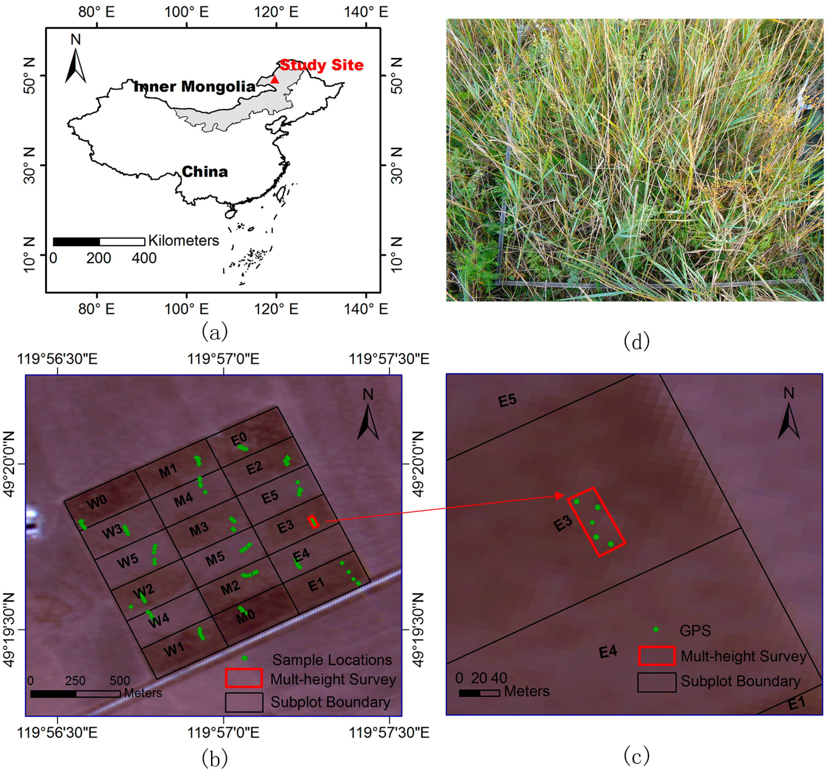
2.1. Study Area
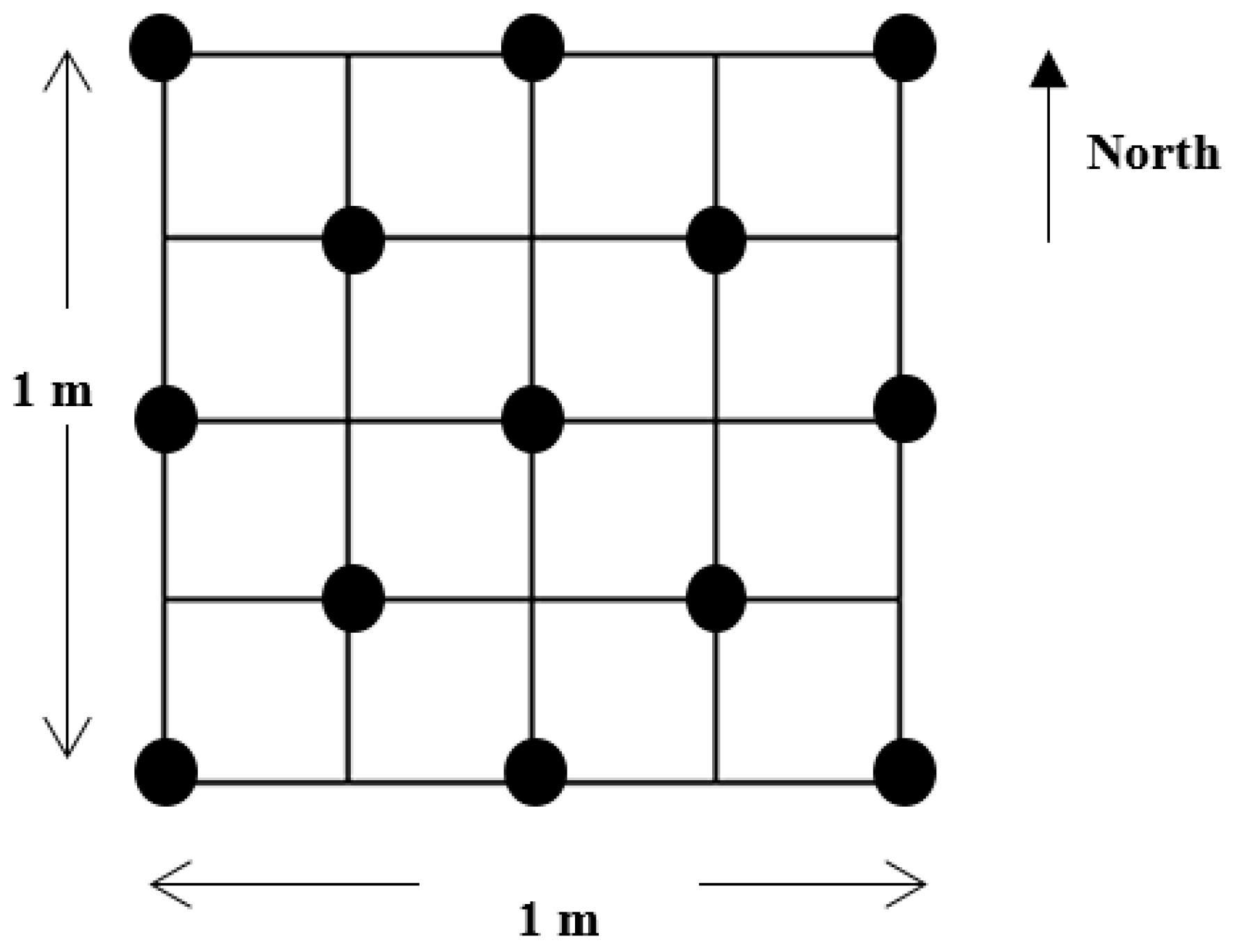
2.2. Field Vegetation Measurements
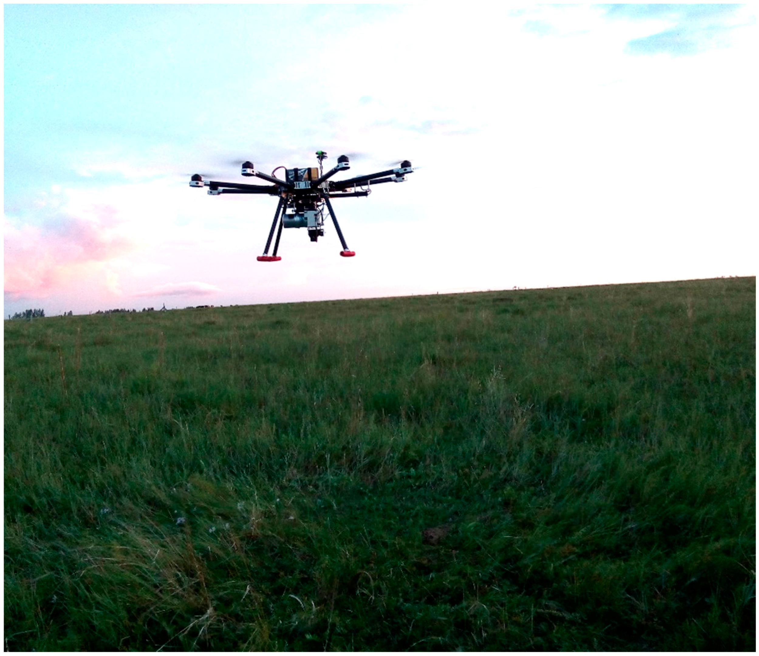
2.3. Light Detection and Ranging (Lidar) Data Collection and Pre-Processing
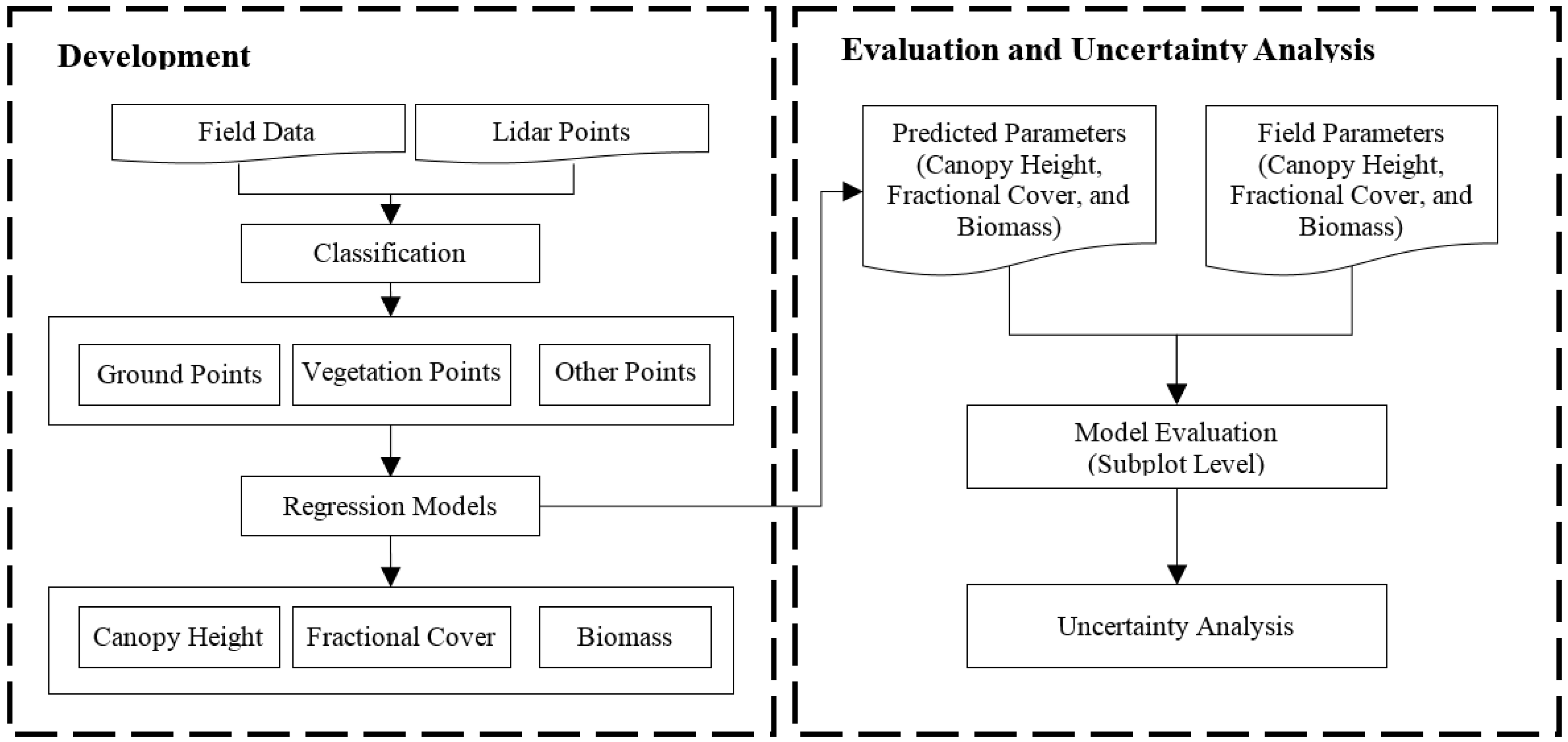
2.4. Parameter Estimation and Mapping
2.5. Influence of Flight Height
3. Results
3.1. Analysis of Field Measurements
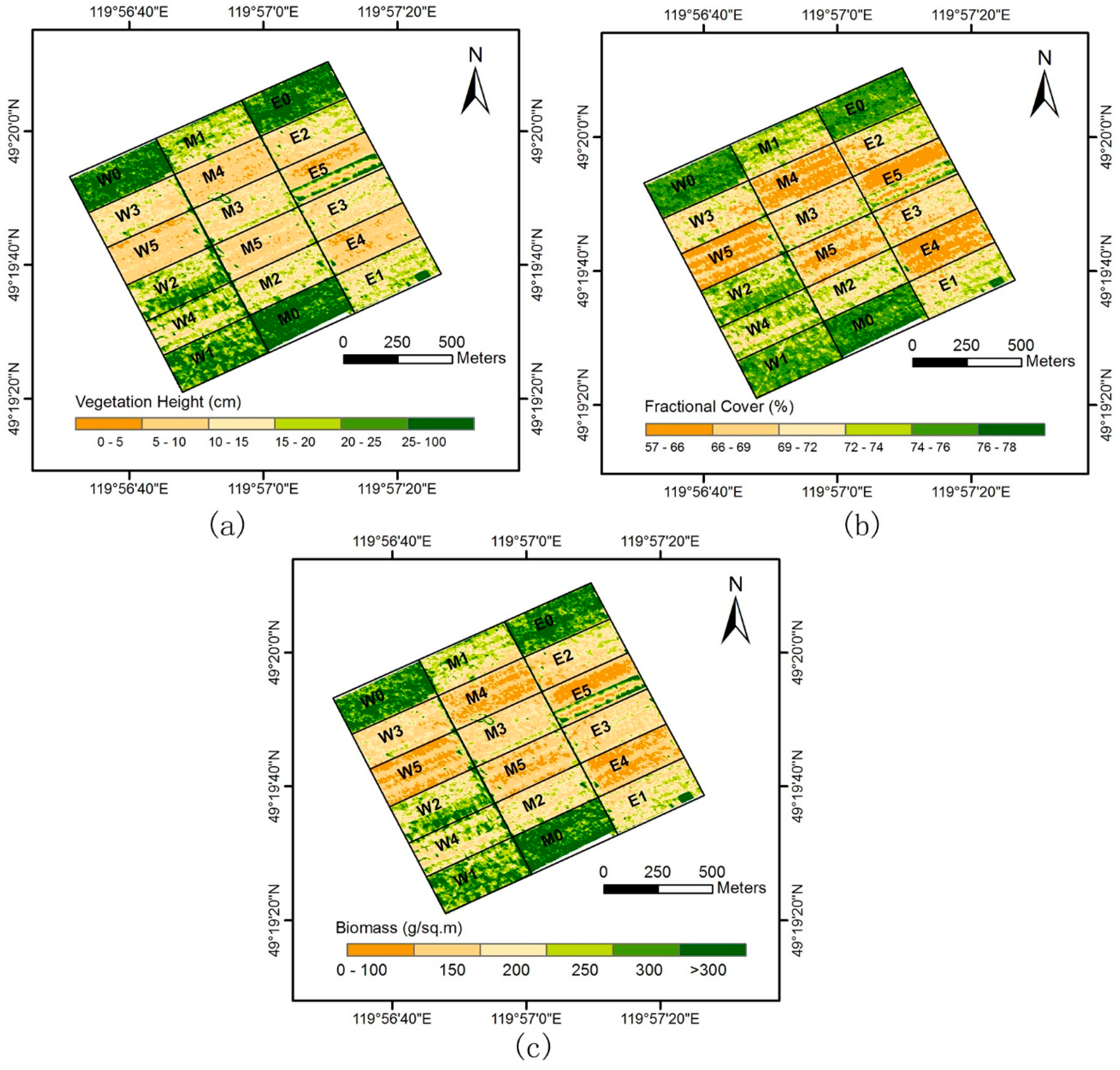
3.2. Lidar-Derived Parameters
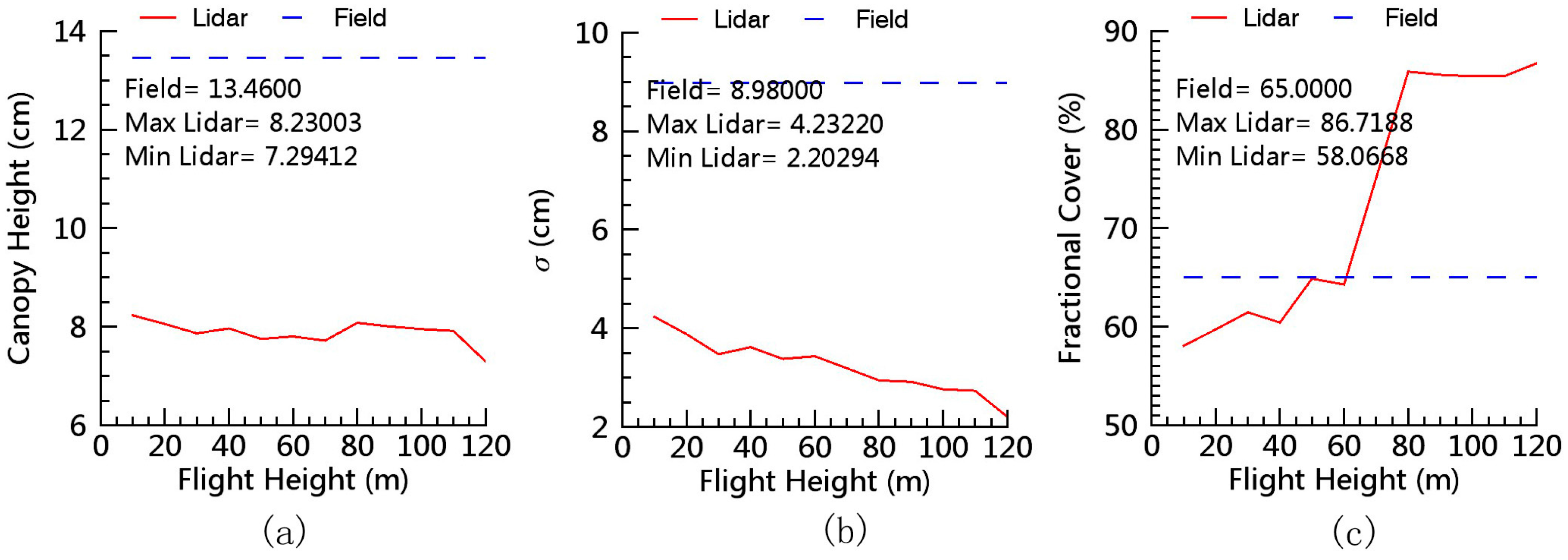
3.3. Influence of Flight Height
4. Discussion
4.1. Advantages
- (1)
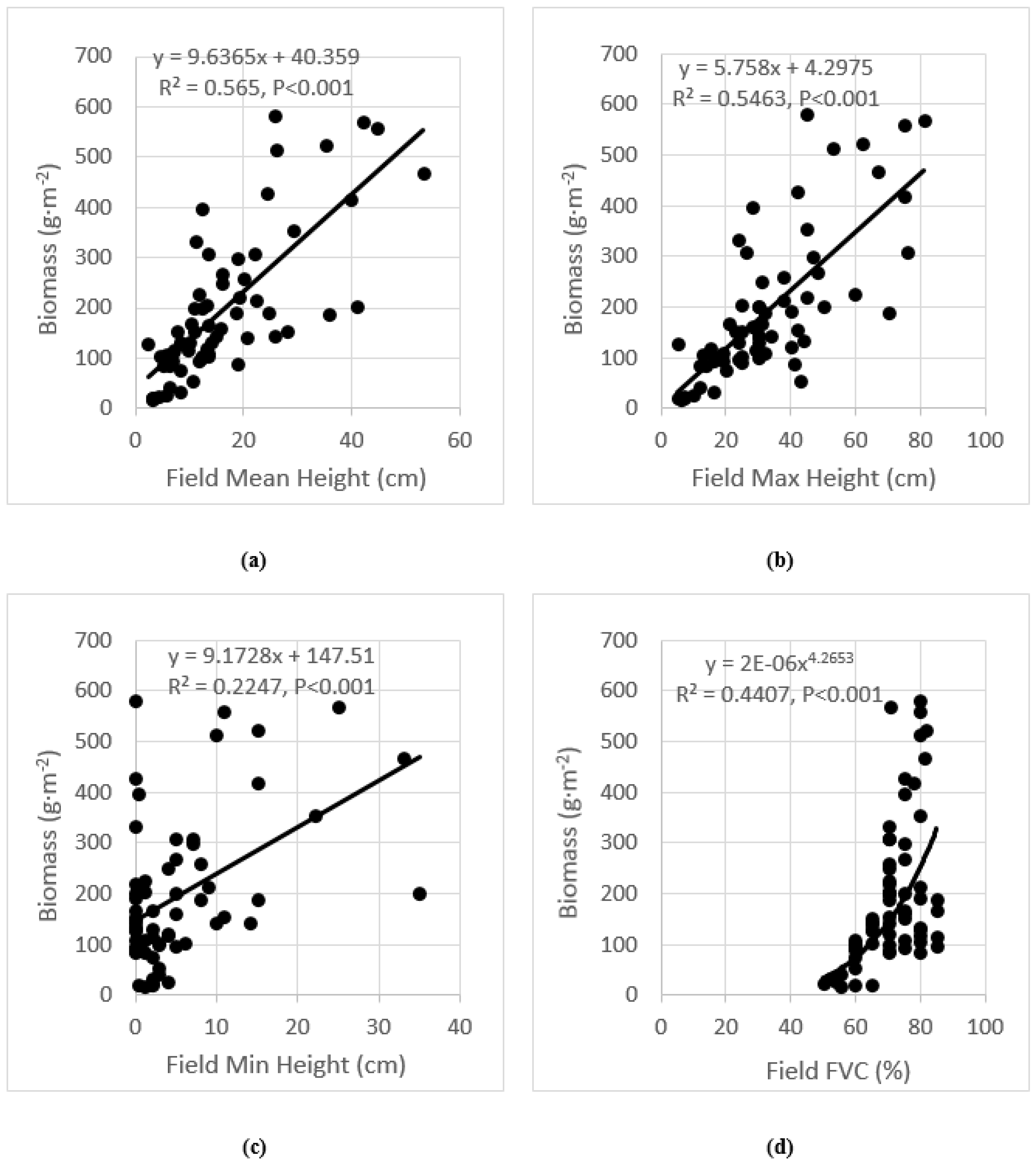
- The changes in canopy height or cover are remarkable. Previous researchers have reported that VI-based optical remote sensing has a severe saturation problem on the estimation of biomass in grasslands with high canopy cover or leaf area index because of the limited capability of detecting canopy height [2,21]. Backscatter-based SAR sensors are less sensitive to the change in canopy structure parameters and biomass for short vegetation, such as grasses [28,29]. However, lidar can directly measure the three-dimensional aspects of vegetation canopy. A combination of lidar-derived canopy height and fractional cover has been shown to accurately estimate aboveground biomass even in high biomass ecosystems, where passive optical and active microwave sensors typically suffer saturation problems [33,34]. This study also demonstrates a high accuracy for estimating the biomass with the mean canopy height varying from 6 cm to 33.7 cm (Figure 7 and Table 4).
- (2)
- A significant amount of dead vegetation exists (e.g., the grassland during non-growing seasons). VI-based optical and backscatter-based SAR sensors depend heavily on vegetation chlorophyll and water contents [2,20], and exhibit high uncertainty in monitoring the non-growing season vegetation [50]. However, lidar discrete-return range data is independent from vegetation chlorophyll and water content, because the lidar sensor itself illuminates the objects and can obtain directly the 3D canopy structure information. Consequently, lidar data is the most suitable remotely sensed data for measuring canopy structure parameters and biomass regardless of the vegetation is alive or dead. This is very important for grassland managers to monitor the non-growing season grasslands, because non-growing seasons typically account for nearly three-quarters of a year [42], and the forage remaining is the main food source for livestock and wild animals to last the non-growing seasons.
4.2. Error Sources
5. Conclusions
Acknowledgments
Author Contributions
Conflicts of Interest
References
- Rango, A.; Laliberte, A.; Herrick, J.E.; Winters, C.; Havstad, K.; Steele, C.; Browning, D. Unmanned aerial vehicle-based remote sensing for rangeland assessment, monitoring, and management. J. Appl. Remote Sens. 2009, 3, 033542. [Google Scholar]
- Jin, Y.; Yang, X.; Qiu, J.; Li, J.; Gao, T.; Wu, Q.; Zhao, F.; Ma, H.; Yu, H.; Xu, B. Remote sensing-based biomass estimation and its spatio-temporal variations in temperate grassland, Northern China. Remote Sens. 2014, 6, 1496–1513. [Google Scholar] [CrossRef]
- Feng, X.; Fu, B.; Lu, N.; Zeng, Y.; Wu, B. How ecological restoration alters ecosystem services: An analysis of carbon sequestration in China’s loess plateau. Sci. Rep. 2013, 3, 2846. [Google Scholar] [CrossRef] [PubMed]
- Brown, L. Grasslands. In The Audubon Society Nature Guides; Alfred A Knopf, Inc.: New York, NY, USA, 1989. [Google Scholar]
- Rogers, J.N.; Parrish, C.E.; Ward, L.G.; Burdick, D.M. Evaluation of field-measured vertical obscuration and full waveform lidar to assess salt marsh vegetation biophysical parameters. Remote Sens. Environ. 2015, 156, 264–275. [Google Scholar] [CrossRef]
- Li, F.; Zeng, Y.; Luo, J.; Ma, R.; Wu, B. Modeling grassland aboveground biomass using a pure vegetation index. Ecol. Indic. 2016, 62, 279–288. [Google Scholar] [CrossRef]
- Okin, G.S. A new model of wind erosion in the presence of vegetation. J. Geophys. Res. Atmos. 2008, 113, 1–11. [Google Scholar] [CrossRef]
- Fan, J.; Zhong, H.; Harris, W.; Yu, G.; Wang, S.; Hu, Z.; Yue, Y. Carbon storage in the grasslands of China based on field measurements of above- and below-ground biomass. Clim. Chang. 2008, 86, 375–396. [Google Scholar] [CrossRef]
- Ni, J. Estimating net primary productivity of grasslands from field biomass measurements in temperate Northern China. Plant Ecol. 2004, 174, 217–234. [Google Scholar] [CrossRef]
- Azzari, G.; Goulden, M.L.; Rusu, R.B. Rapid characterization of vegetation structure with a microsoft kinect sensor. Sensors 2013, 13, 2384–2398. [Google Scholar] [CrossRef] [PubMed]
- Richardson, J.J.; Moskal, L.M.; Bakker, J.D. Terrestrial laser scanning for vegetation sampling. Sensors 2014, 14, 20304–20319. [Google Scholar] [CrossRef] [PubMed]
- Sakowska, K.; Gianelle, D.; Zaldei, A.; MacArthur, A.; Carotenuto, F.; Miglietta, F.; Zampedri, R.; Cavagna, M.; Vescovo, L. Whiteref: A new tower-based hyperspectral system for continuous reflectance measurements. Sensors 2015, 15, 1088–1105. [Google Scholar] [CrossRef] [PubMed]
- Jia, K.; Liang, S.; Gu, X.; Baret, F.; Wei, X.; Wang, X.; Yao, Y.; Yang, L.; Li, Y. Fractional vegetation cover estimation algorithm for Chinese GF-1 wide field view data. Remote Sens. Environ. 2016, 177, 184–191. [Google Scholar] [CrossRef]
- Jia, W.; Liu, M.; Yang, Y.; He, H.; Zhu, X.; Yang, F.; Yin, C.; Xiang, W. Estimation and uncertainty analyses of grassland biomass in Northern China: Comparison of multiple remote sensing data sources and modeling approaches. Ecol. Indic. 2016, 60, 1031–1040. [Google Scholar] [CrossRef]
- Xu, D.; Guo, X. Some insights on grassland health assessment based on remote sensing. Sensors 2015, 15, 3070–3089. [Google Scholar] [CrossRef] [PubMed]
- Piao, S.; Fang, J.; Zhou, L.; Tan, K.; Tao, S. Changes in biomass carbon stocks in China’s grasslands between 1982 and 1999. Glob. Biogeochem. Cycles 2007, 21, 1–10. [Google Scholar] [CrossRef]
- Hill, M.J.; Donald, G.E.; Vickery, P.J. Relating radar backscatter to biophysical properties of temperate perennial grassland. Remote Sens. Environ. 1999, 67, 15–31. [Google Scholar] [CrossRef]
- Marabel, M.; Alvarez-Taboada, F. Spectroscopic determination of aboveground biomass in grasslands using spectral transformations, support vector machine and partial least squares regression. Sensors 2013, 13, 10027–10051. [Google Scholar] [CrossRef] [PubMed]
- Scotta, F.C.; da Fonseca, E.L. Multiscale trend analysis for pampa grasslands using ground data and vegetation sensor imagery. Sensors 2015, 15, 17666–17692. [Google Scholar] [CrossRef] [PubMed]
- Gillan, J.K.; Karl, J.W.; Duniway, M.; Elaksher, A. Modeling vegetation heights from high resolution stereo aerial photography: An application for broad-scale rangeland monitoring. J. Environ. Manag. 2014, 144, 226–235. [Google Scholar] [CrossRef] [PubMed]
- Chen, J.; Gu, S.; Shen, M.; Tang, Y.; Matsushita, B. Estimating aboveground biomass of grassland having a high canopy cover: An exploratory analysis of in situ hyperspectral data. Int. J. Remote Sens. 2009, 30, 6497–6517. [Google Scholar] [CrossRef]
- Ni, W.; Ranson, K.J.; Zhang, Z.; Sun, G. Features of point clouds synthesized from multi-view ALOS/PRISM data and comparisons with LiDAR data in forested areas. Remote Sens. Environ. 2014, 149, 47–57. [Google Scholar] [CrossRef]
- Balzter, H.; Rowland, C.S.; Saich, P. Forest canopy height and carbon estimation at monks wood national nature reserve, UK, using dual-wavelength sar interferometry. Remote Sens. Environ. 2007, 108, 224–239. [Google Scholar] [CrossRef]
- Cartus, O.; Santoro, M.; Kellndorfer, J. Mapping forest aboveground biomass in the northeastern united states with alos palsar dual-polarization L-band. Remote Sens. Environ. 2012, 124, 466–478. [Google Scholar] [CrossRef]
- Renaudin, E.; Mercer, B. Forest biomass derivation from single pass dual baseline polarisation coherence tomography. In Proceedings of the 2012 IEEE International Geoscience and Remote Sensing Symposium (IGARSS), Munich, Germany, 22–27 July 2012; pp. 479–482.
- Cloude, S.R. Polarization coherence tomography. Radio Sci. 2006, 41, 4017. [Google Scholar] [CrossRef]
- Michelakis, D.; Stuart, N.; Brolly, M.; Woodhouse, I.H.; Lopez, G.; Linares, V. Estimation of woody biomass of pine savanna woodlands from ALOS PALSAR imagery. IEEE J. Sel. Top. Appl. Earth Observ. Remote Sens. 2015, 8, 244–254. [Google Scholar] [CrossRef]
- Voormansik, K.; Jagdhuber, T.; Olesk, A.; Hajnsek, I.; Papathanassiou, K.P. Towards a detection of grassland cutting practices with dual polarimetric terrasar-X data. Int. J. Remote Sens. 2013, 34, 8081–8103. [Google Scholar] [CrossRef]
- Schuster, C.; Ali, I.; Lohmann, P.; Frick, A.; Forster, M.; Kleinschmit, B. Towards detecting swath events in terrasar-X time series to establish natura 2000 grassland habitat swath management as monitoring parameter. Remote Sens. 2012, 4, 2455–2456. [Google Scholar] [CrossRef]
- Lee, Y.-K.; Park, J.-W.; Choi, J.-K.; Oh, Y.; Won, J.-S. Potential uses of terrasar-X for mapping herbaceous halophytes over salt marsh and tidal flats. Estuar. Coast. Shelf Sci. 2012, 115, 366–376. [Google Scholar] [CrossRef]
- Mitchell, J.J.; Shrestha, R.; Spaete, L.P.; Glenn, N.F. Combining airborne hyperspectral and lidar data across local sites for upscaling shrubland structural information: Lessons for hyspiri. Remote Sens. Environ. 2015, 167, 98–110. [Google Scholar] [CrossRef]
- Olsoy, P.J.; Glenn, N.F.; Clark, P.E. Estimating sagebrush biomass using terrestrial laser scanning. Rangel. Ecol. Manag. 2014, 67, 224–228. [Google Scholar] [CrossRef]
- Gwenzi, D.; Lefsky, M.A. Modeling canopy height in a savanna ecosystem using spacebome lidar waveforms. Remote Sens. Environ. 2014, 154, 338–344. [Google Scholar] [CrossRef]
- Wasser, L.; Day, R.; Chasmer, L.; Taylor, A. Influence of vegetation structure on lidar-derived canopy height and fractional cover in forested riparian buffers during leaf-off and leaf-on conditions. PLoS ONE 2013, 8, e54776. [Google Scholar] [CrossRef] [PubMed]
- Lefsky, M.A.; Cohen, W.B.; Harding, D.J.; Parker, G.G.; Acker, S.A.; Gower, S.T. Lidar remote sensing of above-ground biomass in three biomes. Glob. Ecol. Biogeogr. 2002, 11, 393–399. [Google Scholar] [CrossRef]
- Reddy, A.D.; Hawbaker, T.J.; Wurster, F.; Zhu, Z.; Ward, S.; Newcomb, D.; Murray, R. Quantifying soil carbon loss and uncertainty from a peatland wildfire using multi-temporal lidar. Remote Sens. Environ. 2015, 170, 306–316. [Google Scholar] [CrossRef]
- Lefsky, M.A. A global forest canopy height map from the moderate resolution imaging spectroradiometer and the geoscience laser altimeter system. Geophys. Res. Lett. 2010, 37, 78–82. [Google Scholar] [CrossRef]
- Dubayah, R.O.; Sheldon, S.L.; Clark, D.B.; Hofton, M.A.; Blair, J.B.; Hurtt, G.C.; Chazdon, R.L. Estimation of tropical forest height and biomass dynamics using lidar remote sensing at La Selva, Costa Rica. J. Geophys. Res. Biogeosci. 2010, 115, 272–281. [Google Scholar] [CrossRef]
- Bork, E.W.; Su, J.G. Integrating lidar data and multispectral imagery for enhanced classification of rangeland vegetation: A meta analysis. Remote Sens. Environ. 2007, 111, 11–24. [Google Scholar] [CrossRef]
- Wallace, L.; Lucieer, A.; Watson, C.S. Evaluating tree detection and segmentation routines on very high resolution UAV LiDAR data. IEEE Trans. Geosci. Remote Sens. 2014, 52, 7619–7628. [Google Scholar] [CrossRef]
- Wallace, L.; Lucieer, A.; Malenovský, Z.; Turner, D.; Vopěnka, P. Assessment of forest structure using two uav techniques: A comparison of airborne laser scanning and structure from motion (SFM) point clouds. Forests 2016, 7, 62. [Google Scholar] [CrossRef]
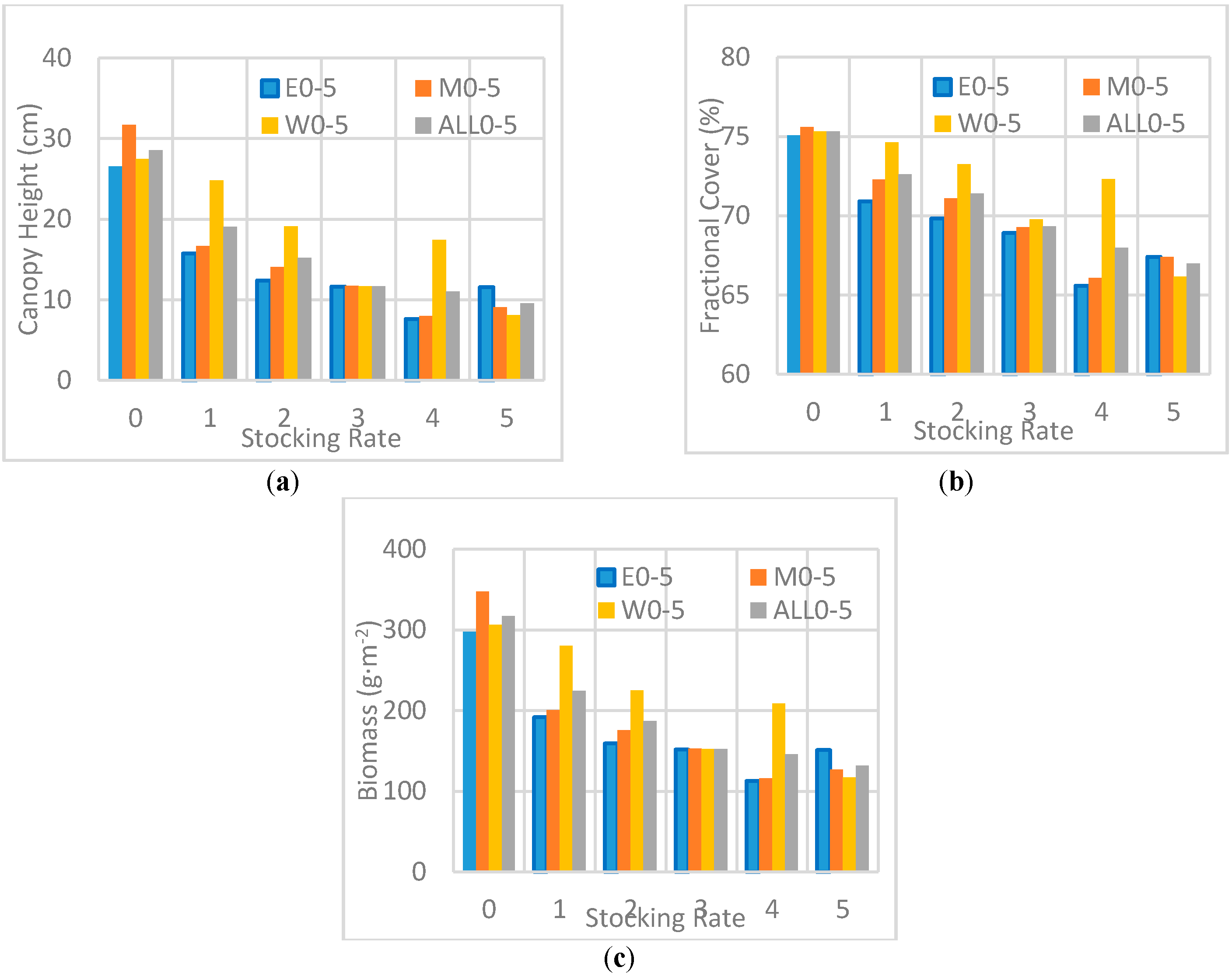
- Yan, R.; Xin, X.; Yan, Y.; Wang, X.; Zhang, B.; Yang, G.; Liu, S.; Deng, Y.; Li, L. Impacts of differing grazing rates on canopy structure and species composition in hulunber meadow steppe. Rangel. Ecol. Manag. 2015, 68, 54–64. [Google Scholar] [CrossRef]
- Middleton, J.H.; Cooke, C.G.; Kearney, E.T.; Mumford, P.J.; Mole, M.A.; Nippard, G.J.; Rizos, C.; Splinter, K.D.; Turner, I.L. Resolution and accuracy of an airborne scanning laser system for beach surveys. J. Atmos. Ocean. Technol. 2013, 30, 2452–2464. [Google Scholar] [CrossRef]
- Tulldahl, H.M.; Bissmarck, F.; Larsson, H.; Grönwall, C.; Tolt, G. Accuracy evaluation of 3D lidar data from small UAV. In Proceedings of the SPIE Conference on Electro-Optical Remote Sensing, Photonic Technologies, and Applications IX, Toulouse, France, 21–22 September 2015; pp. 964903–964911.
- Maas, H.G.; Vosselman, G. Two algorithms for extracting building models from raw laser altimetry data. ISPRS J. Photogramm. Remote Sens. 1999, 54, 153–163. [Google Scholar] [CrossRef]
- Axelsson, P. DEM generation from laser scanner data using adaptive TIN models. Int. Arch. Photogramm. Remote Sens. 2000, 33, 111–118. [Google Scholar]
- Morris, J.T.; Haskin, B. A 5-yr record of aerial primary production and stand characteristics of spartina alterniflora. Ecology 1990, 71, 2209–2217. [Google Scholar] [CrossRef]
- Möller, I. Quantifying saltmarsh vegetation and its effect on wave height dissipation: Results from a UK east coast saltmarsh. Estuar. Coast. Shelf Sci. 2006, 69, 337–351. [Google Scholar] [CrossRef]
- Ni-Meister, W.; Lee, S.; Strahler, A.H.; Woodcock, C.E.; Schaaf, C.; Yao, T.; Ranson, K.J.; Sun, G.; Blair, J.B. Assessing general relationships between aboveground biomass and vegetation structure parameters for improved carbon estimate from lidar remote sensing. J. Geophys. Res. Atmos. 2010, 115, 79–89. [Google Scholar] [CrossRef]
- Tagesson, T. Using earth observation-based dry season NDVI trends for assessment of changes in tree cover in the Sahel. Int. J. Remote Sens. 2014, 35, 2493–2515. [Google Scholar]
- Li, F.; Cui, X.; Liu, X.; Wei, A.; Wu, Y. Positioning errors analysis on airborne lidar point clouds. Infrared Laser Eng. 2014, 43, 1842–1849. [Google Scholar]
- Naesset, E. Effects of different sensors, flying altitudes, and pulse repetition frequencies on forest canopy metrics and biophysical stand properties derived from small-footprint airborne laser data. Remote Sens. Environ. 2009, 113, 148–159. [Google Scholar] [CrossRef]
- Hladik, C.; Schalles, J.; Alber, M. Salt marsh elevation and habitat mapping using hyperspectral and lidar data. Remote Sens. Environ. 2013, 139, 318–330. [Google Scholar] [CrossRef]
- Tang, H.; Dubayah, R.; Swatantran, A.; Hofton, M.; Sheldon, S.; Clark, D.B.; Blair, B. Retrieval of vertical LAI profiles over tropical rain forests using waveform lidar at La Selva, Costa Rica. Remote Sens. Environ. 2012, 124, 242–250. [Google Scholar] [CrossRef]
- Tang, H.; Brolly, M.; Zhao, F.; Strahler, A.H.; Schaaf, C.L.; Ganguly, S.; Zhang, G.; Dubayah, R. Deriving and validating Leaf Area Index (LAI) at multiple spatial scales through lidar remote sensing: A case study in Sierra National Forest, CA. Remote Sens. Environ. 2014, 143, 131–141. [Google Scholar] [CrossRef]
- Nayegandhi, A.; Brock, J.C.; Wright, C.W. Small-footprint, waveform-resolving lidar estimation of submerged and sub-canopy topography in coastal environments. Int. J. Remote Sens. 2009, 30, 861–878. [Google Scholar] [CrossRef]


| Subplot No. | Mean Canopy Height (cm) | Mean Fractional Cover (%) | Mean Biomass (g·m−2) | |||
|---|---|---|---|---|---|---|
| Subplot Level | Grazing Rate Level | Subplot Level | Grazing Rate Level | Subplot Level | Grazing Rate Level | |
| W0 | 38.0 | 33.7 | 78.6 | 76.5 | 528.2 | 391.2 |
| M0 | 30.4 | 74 | 180.0 | |||
| W0 | 32.7 | 76.8 | 465.3 | |||
| E1 | 27.3 | 21.2 | 81 | 75 | 195.7 | 211.8 |
| M1 | 20.5 | 73 | 299.2 | |||
| W1 | 16.0 | 71 | 140.5 | |||
| E2 | 13.6 | 12.2 | 72 | 77 | 134.0 | 144.7 |
| M2 | 10.6 | 81 | 150.5 | |||
| W2 | 12.5 | 78 | 149.7 | |||
| E3 | 13.5 | 13.7 | 68 | 69.7 | 180.6 | 239.2 |
| M3 | 16.4 | 70 | 225.1 | |||
| W3 | 11.3 | 71 | 312.0 | |||
| E4 | 5.2 | 6.8 | 69 | 63.7 | 121.1 | 101.9 |
| M4 | 4.9 | 58 | 83.2 | |||
| W4 | 10.2 | 64 | 101.5 | |||
| E5 | 8.2 | 6.0 | 57.6 | 62.4 | 59.7 | 56.0 |
| M5 | 4.9 | 57.6 | 28.6 | |||
| W5 | 4.9 | 72 | 82.7 | |||
| Flight Parameter | Value |
|---|---|
| Flying speed | 5 m/s |
| Flight height | 10–120 m at intervals of 10 m (survey #1) |
| 40 m (survey #2) | |
| Laser beam divergence | 3 mrad |
| Wavelength | 903 nm |
| Rotation rate | 5 Hz |
| Scan angle | +10° to −30° (+5° to −5° remained) |
| Point density | 26 pts/m2 |
| Laser footprint | 0.12 m (40 m range) |
| Independent Variable (x) | Dependent Variable (y) | Model | R2 | RMSE | rRMSE (%) | p |
|---|---|---|---|---|---|---|
| Lidar mean height | Field mean height | y = 3.557x − 3.167 | 0.583 | 4.9 cm | 9.4 | <0.001 |
| Lidar max height | Field max height | y = 0.801x + 14.74 | 0.201 | 10.6 cm | 13.1 | <0.001 |
| Lidar max height | Field mean height | y = 0.660x + 0.9376 | 0.368 | 17.1 cm | 32.2 | <0.001 |
| Lidar fractional cover | Field fractional cover | y = 0.228x + 54.955 | 0.206 | 4.4% | 5.2 | <0.001 |
| Independent Variable (x) | Model | R2 | RMSE (g·m−2) | rRMSE (%) | p |
|---|---|---|---|---|---|
| Lidar mean height | y = 34.785x + 7.081 | 0.340 | 81.89 | 14.1% | <0.001 |
| Lidar max height | y = 5.522x + 68.397 | 0.157 | 87.96 | 15.1% | <0.001 |
| Lidar FVC | y = 22.842e0.0266x | 0.316 | 90.18 | 15.5% | <0.001 |
| Lidar mean height (x1) + Lidar FVC (x2) | y = 35.087x1 − 0.0467x2 + 8.711 | 0.341 | 81.85 | 14.06% | <0.001 |
| Lidar mean height (x1) + Lidar max height (x2) | y = 37.799x1 − 0.958x2 − 12.679 | 0.342 | 87.93 | 15.1% | <0.001 |
| Lidar max height (x1) × Lidar FVC (x2) | y = 1.046x1 + 3.927x2 − 102.860 | 0.276 | 82.07 | 14.1% | <0.001 |
| Lidar-Derived Mean Height | Lidar-Derived Max Height | Lidar-Derived FVC | |
|---|---|---|---|
| Lidar-derived mean height | 1 | - | - |
| Lidar-derived max height | 0.760 | 1 | - |
| Lidar-derived FVC | 0.9584 | 0.696 | 1 |
© 2017 by the authors; licensee MDPI, Basel, Switzerland. This article is an open access article distributed under the terms and conditions of the Creative Commons Attribution (CC-BY) license (http://creativecommons.org/licenses/by/4.0/).
Share and Cite
Wang, D.; Xin, X.; Shao, Q.; Brolly, M.; Zhu, Z.; Chen, J. Modeling Aboveground Biomass in Hulunber Grassland Ecosystem by Using Unmanned Aerial Vehicle Discrete Lidar. Sensors 2017, 17, 180. https://doi.org/10.3390/s17010180
Wang D, Xin X, Shao Q, Brolly M, Zhu Z, Chen J. Modeling Aboveground Biomass in Hulunber Grassland Ecosystem by Using Unmanned Aerial Vehicle Discrete Lidar. Sensors. 2017; 17(1):180. https://doi.org/10.3390/s17010180
Chicago/Turabian StyleWang, Dongliang, Xiaoping Xin, Quanqin Shao, Matthew Brolly, Zhiliang Zhu, and Jin Chen. 2017. "Modeling Aboveground Biomass in Hulunber Grassland Ecosystem by Using Unmanned Aerial Vehicle Discrete Lidar" Sensors 17, no. 1: 180. https://doi.org/10.3390/s17010180