
A Distributed and Energy-Efficient Algorithm for Event K-Coverage in Underwater Sensor Networks

Abstract
:1. Introduction and Related Works
2. Preliminaries: Models and Definitions
2.1. Models
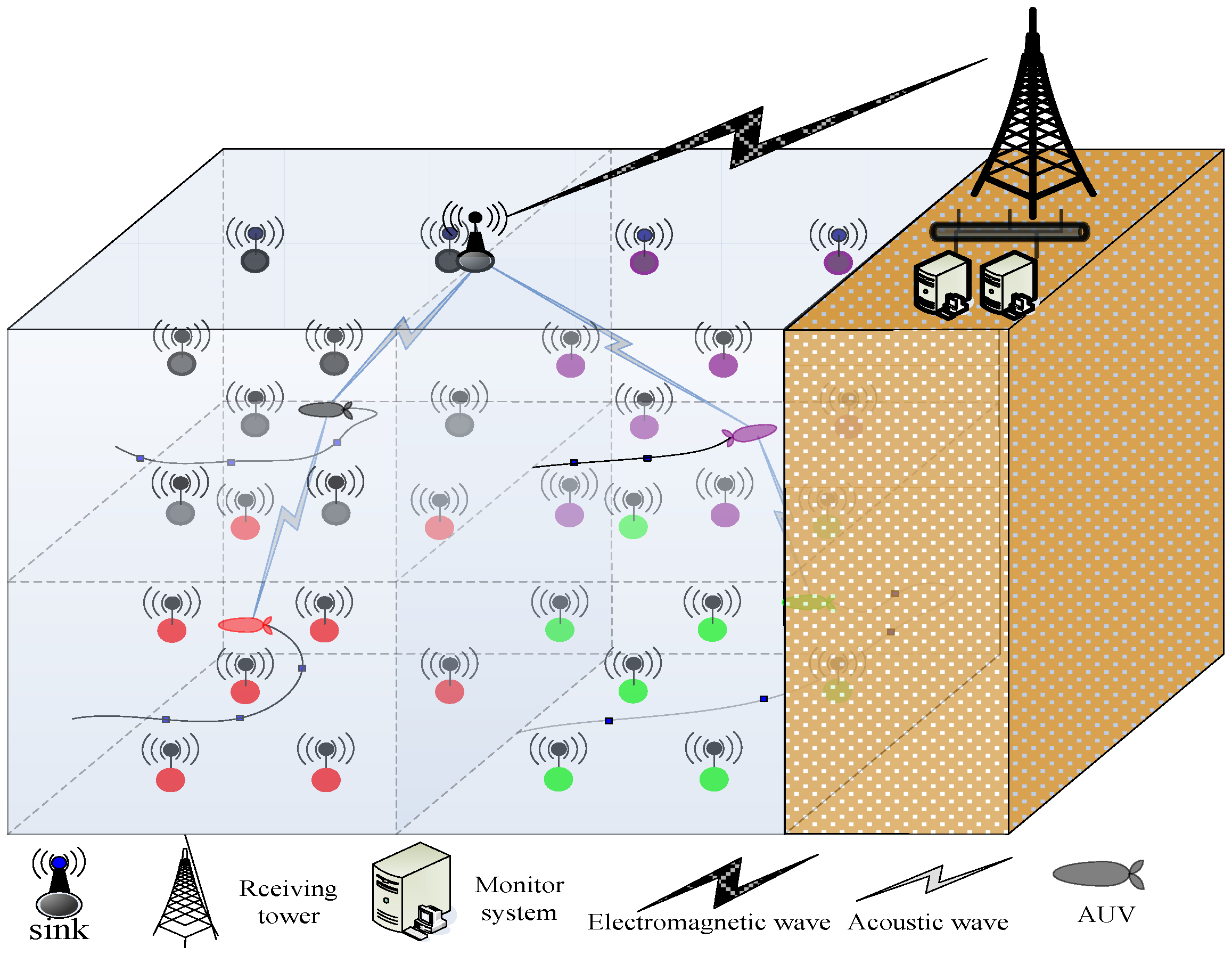
2.1.1. Network Model
- Any node has the ability of communication and perception. Nodes communicate with one another through acoustic channels, and the sink node communicates with the ground monitoring station by radio.
- All nodes are isomorphic before the algorithm runs. Then, the sensing radius of each node can be adjusted between the minimum and maximum sensing radius according to adjustment strategy.
- The position of each event is randomly changed by the water current in the monitoring area but not beyond that. Time interval T is one round of network run. In every round, the algorithm readjusts the sensing radius of some corresponding nodes to achieve K-coverage for all events whose position is changed.
2.1.2. Network Energy Consumption Model
Energy Consumption Model of Communication
Energy Consumption Model of Sensing
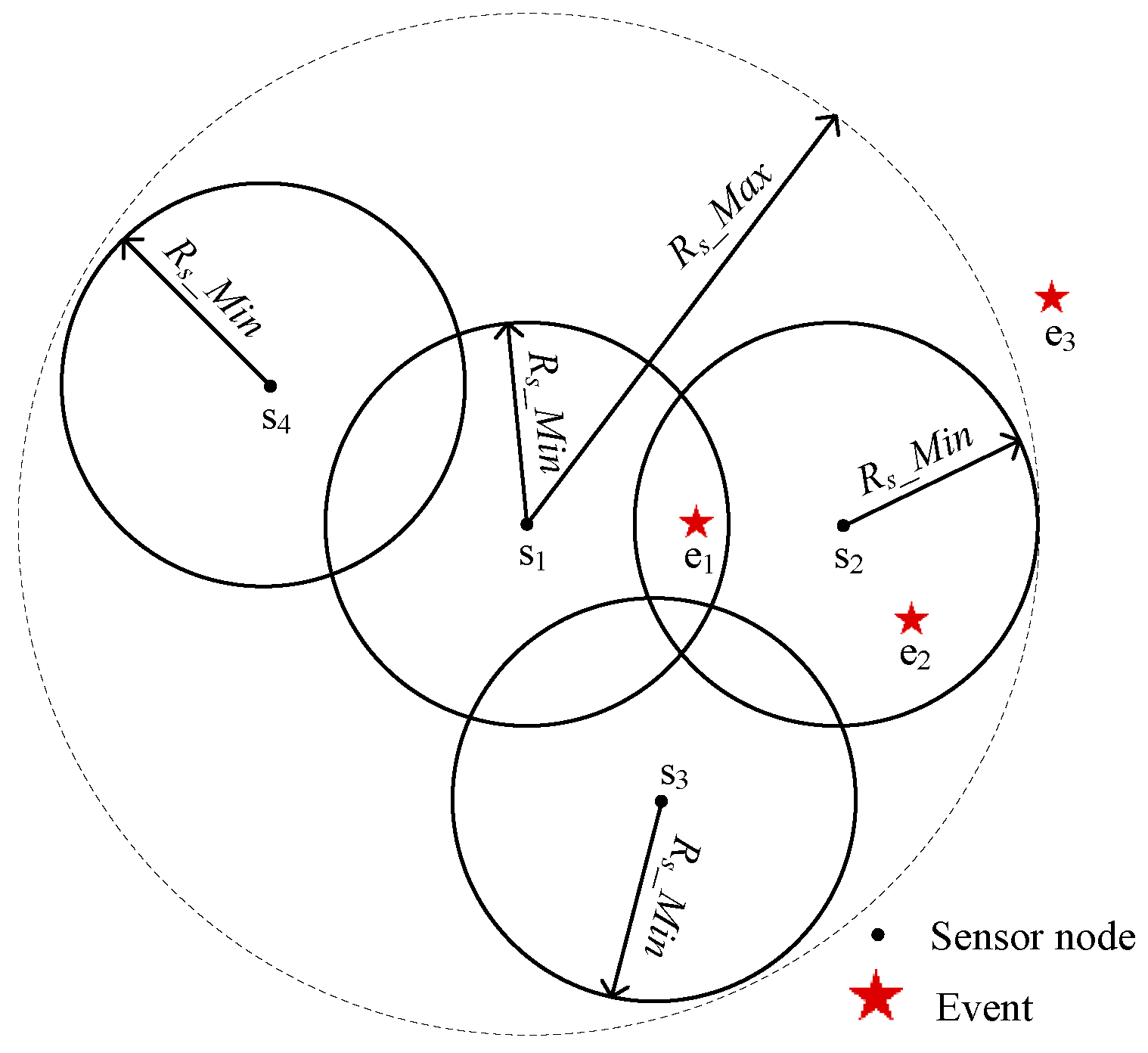
2.1.3. Node Sensing Model
2.1.4. Event Mobility Model
2.2. Definition
2.2.1. Nodes and Events
2.2.2. Event Detection Performance
2.2.3. Network Lifetime
3. Algorithm Description and Process
3.1. Problem Description
3.2. Algorithm Description
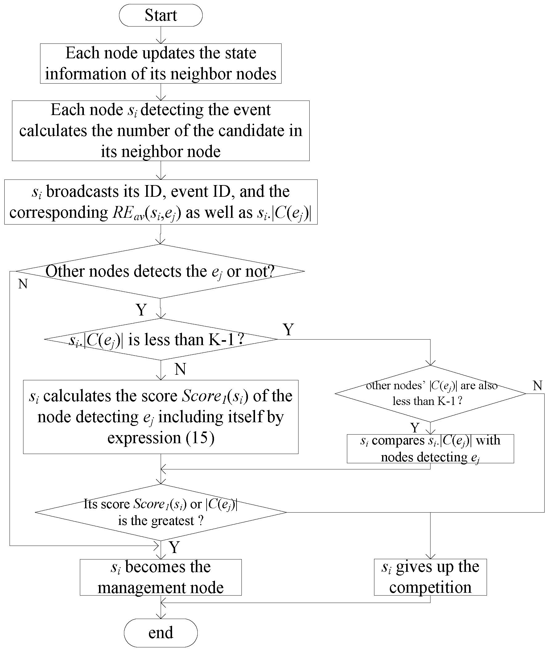
3.2.1. Management Node Formation
- If si.|C(ej)| is less than K − 1 and the candidate node number of the other nodes detecting ej is also less than K − 1, si judges its |C(ej)| among nodes detecting ej. If si.|C(ej)| is not the largest, it automatically gives up the competition of the management node; otherwise, it becomes the management node of ej and joins the management node set M, as well as skips the rest of the process described in this section.
- If si.|C(ej)| is less than K − 1 and the candidate node number of the other nodes detecting ej is not all less than K − 1, si gives up the competition of management node.
- If si.|C(ej)| is greater than K − 1, si then calculates its score Score1(si) and other nodes’ score Score1(sm) by Equation (15). It calculates according to the indicators of the average residual energy of and number of candidate nodes, and the distance to ej. Score1(si) is formulated as follows:where REav(si,ej) is the average residual energy of si’s candidate node for ej, and are the maximum and minimum average residual energy of the candidate node of nodes detecting ej, respectively; dmax and dmin are the maximum and minimum distances to ej, respectively; and are the maximum and minimum numbers of the ej candidate node, respectively.si then compares its score with others. If its score is not the greatest, then si gives up the competition for the management node of ej. Otherwise, si becomes the management node of ej and joins management node set M.
- If the information si receives does not include event ej, which is to say, only si detects ej, si becomes the management node of ej and joins management node set M.
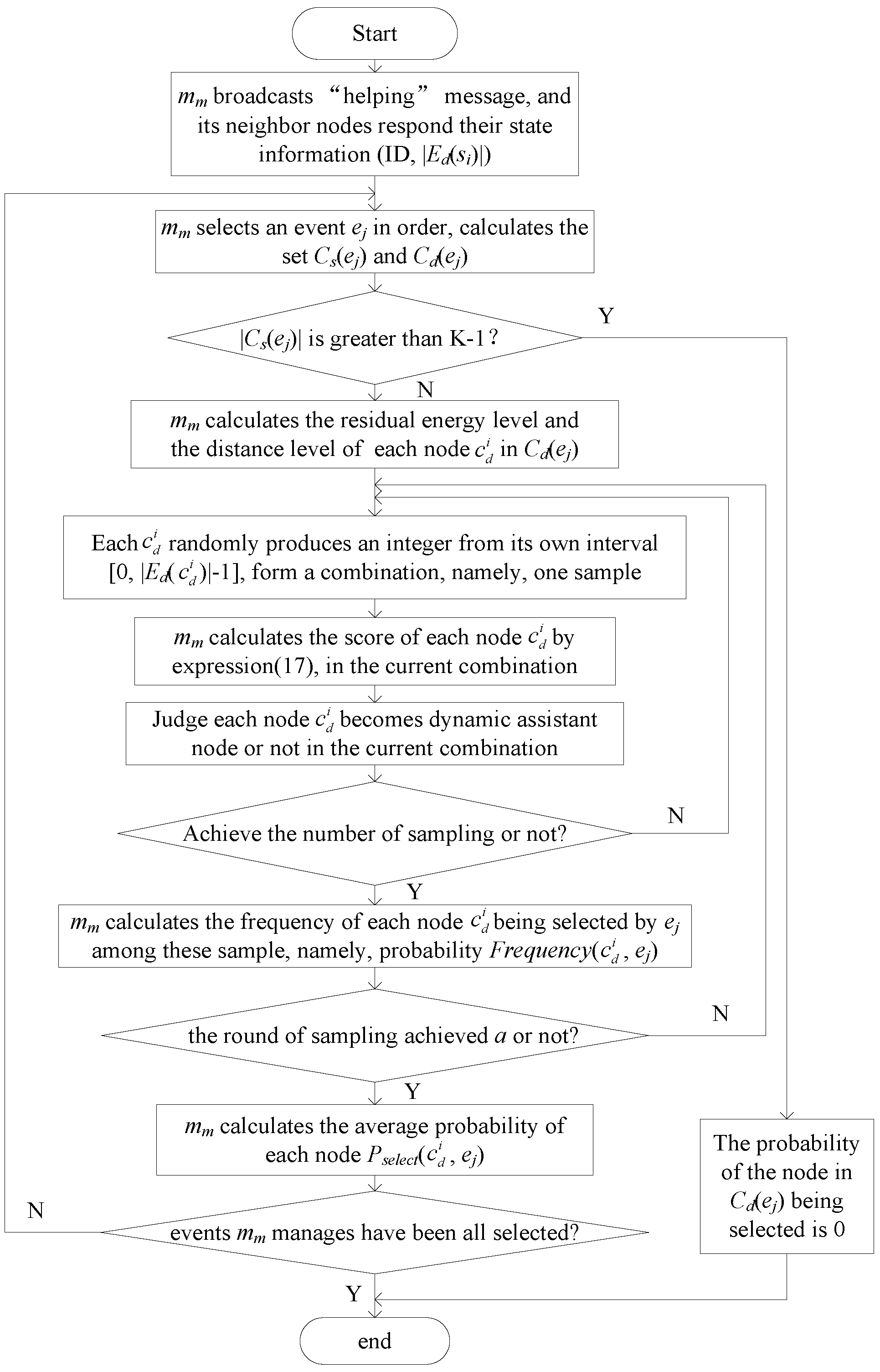
3.2.2. Calculation Probability of Event-Selected Node
- (1)
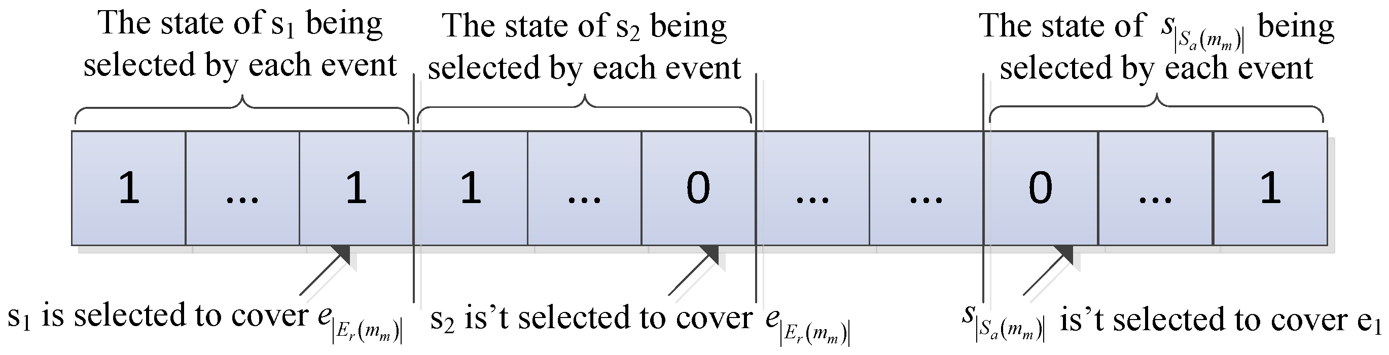
- For each node , mm randomly selects an integer in the interval [0, |Ed()| − 1] as the number of ’s actual dynamic coverage events, and these integers that mm selects form a combination of the number of actual coverage events, namely, one sampling.
- (2)
- mm calculates the score Score2() of each node in the current combination by Equation (17), according to LRE(), Ld(), and :where w1, w2, and w3 are indicator weights whose values are set according to the application focusing on the relevant indicators and w1 + w2 + w3 = 1; and are the minimum and maximum numbers of the actual coverage events in the current combination, respectively.
- (3)
- mm selects K – 1 − nodes as the dynamic assistant nodes of ej, according to the scores in descending order (nodes in must be the assistant nodes of ej because they do not need to increase their sensing radius to cover ej). Other nodes are not selected in the current combination.
- (4)
- If the sample number is less than 400, then Step 1 is repeated. Otherwise, the next step is performed.
- (5)
- For each node , mm records and calculates the frequency of ’s being selected to cover ej Frequency(, ej) in the current round of sampling.
3.2.3. Multi-Objective Optimization Model
Energy Consumption
- (1)
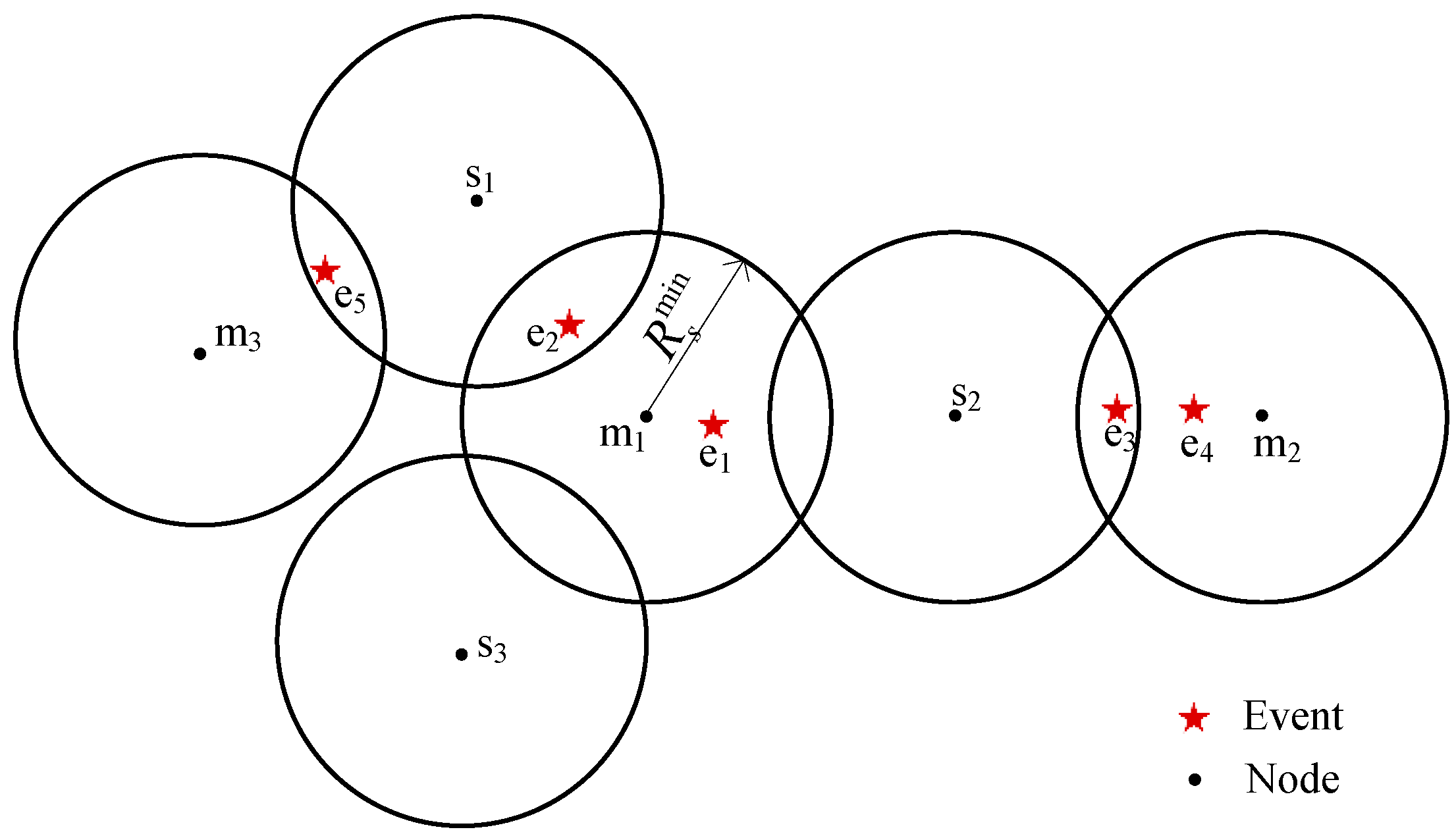
- si dynamically covers one event or more, namely, si dynamically covers the event mm manages, or its is not equal to 0; then, mm calculates the energy consumption of si produced by the cover of these events that mm manages. For example, for the node s2 in Figure 5, its detecting energy consumption is ECS(R2) in the network, but m1 calculates its energy consumption produced by covering e1; in other words, the ECS(R2) is divided into two parts by e1 and e4. Because m1 does not know whether s2 covers e4 or not, in this study, the number of events that other nodes manage and that s2 covers is estimated by the expectation of the actual coverage event number . Therefore, s2’s energy consumption that m1 calculates is .
- (2)
- si only covers some static events, while mm calculates the energy consumption of si produced by the cover of these events that mm manages. In Figure 5, the energy consumption of s1 is ECS() and is divided into two parts by e2 and e5. Because the static cover event number of s1 is definite, the s1’energy consumption m1 calculates is .
- (3)
- si does not cover any event, and the total energy consumption of si is calculated. In Figure 5, s3’s energy consumption m1 calculates ECS().
Residual Energy Variance
Event Detecting Performance
3.2.4. Methodology of the Constrained NSGA-II and Optimization Strategy
- Feasible solutions are greater than non-feasible solutions.
- In non-feasible solutions, the rank of solution with a lower degree of restriction is greater.
4. Algorithm Analysis
4.1. Message Complexity
4.2. Time Complexity
5. Simulation and Performance Analysis
5.1. Simulation Scenario and Parameter Settings
5.2. Simulation Example
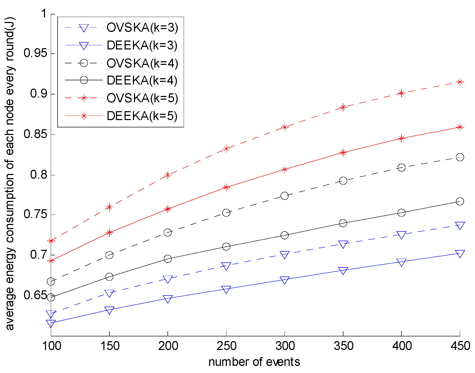
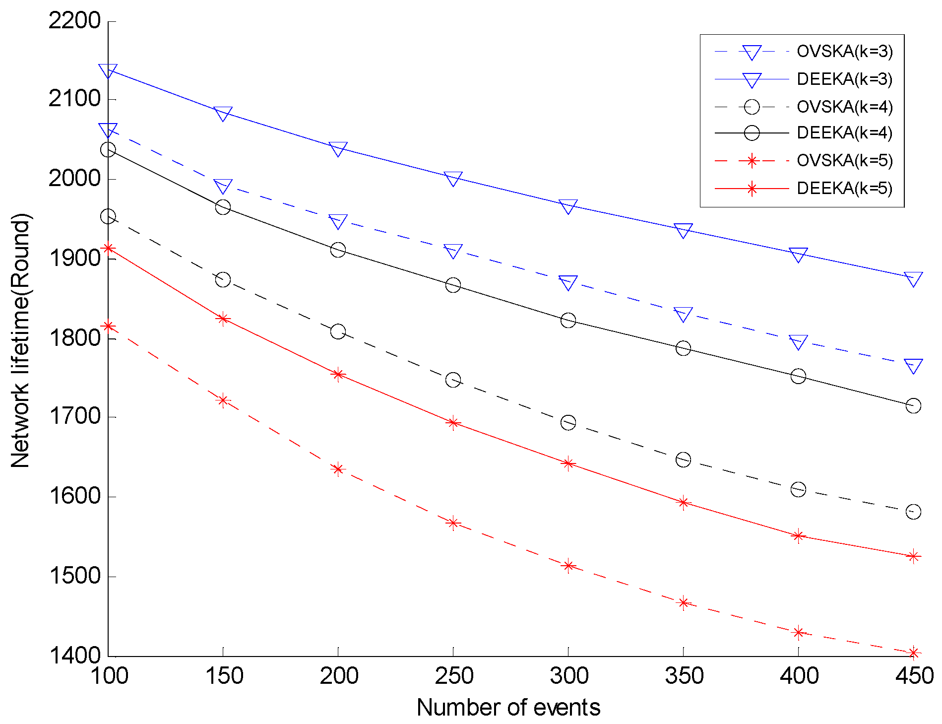
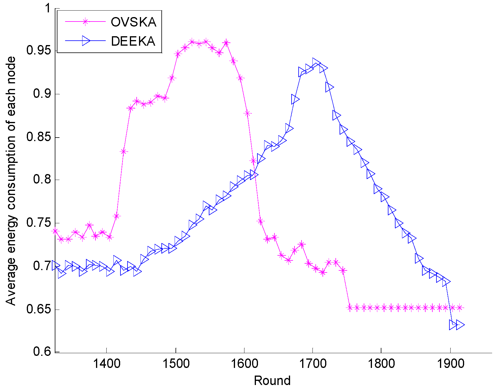
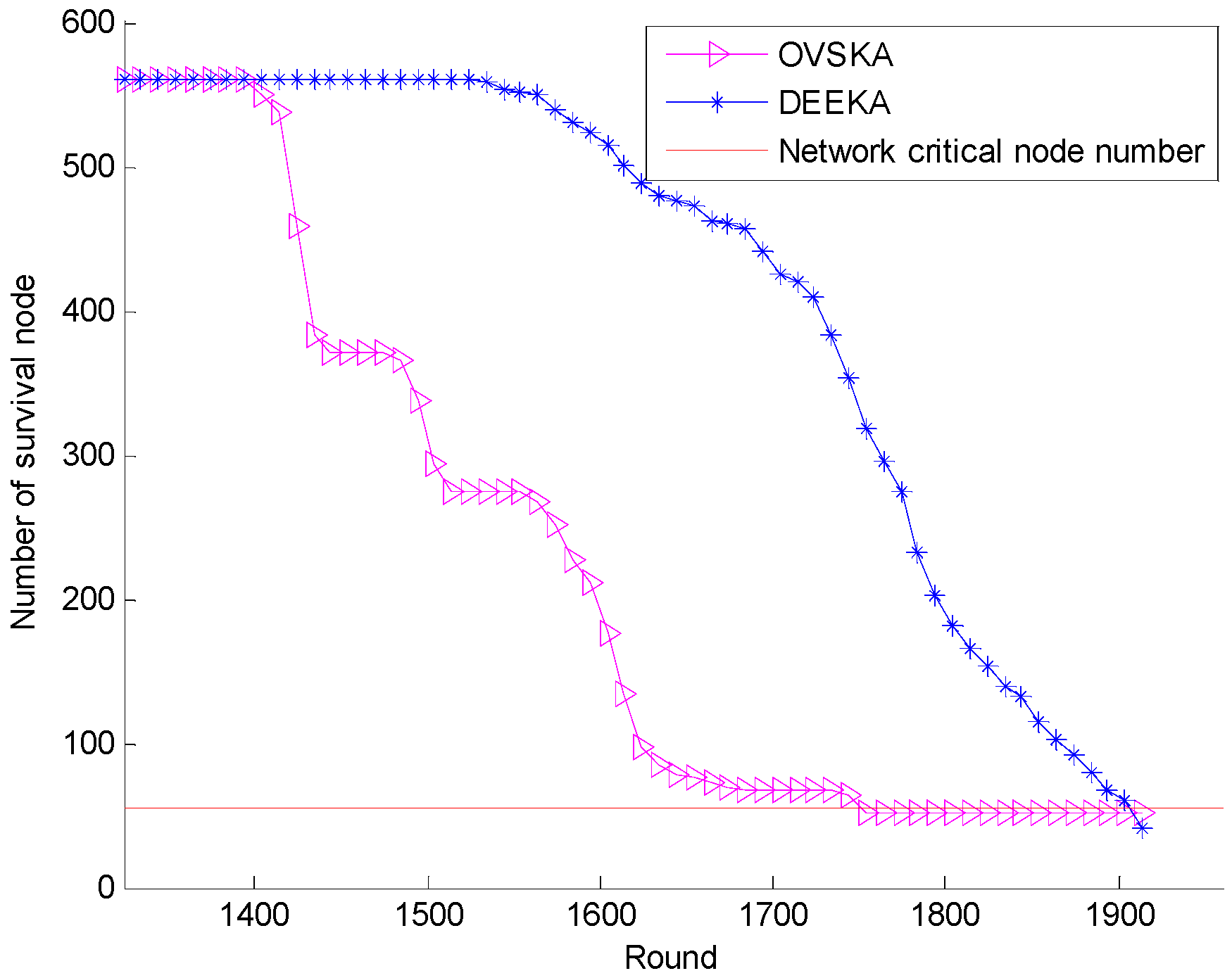
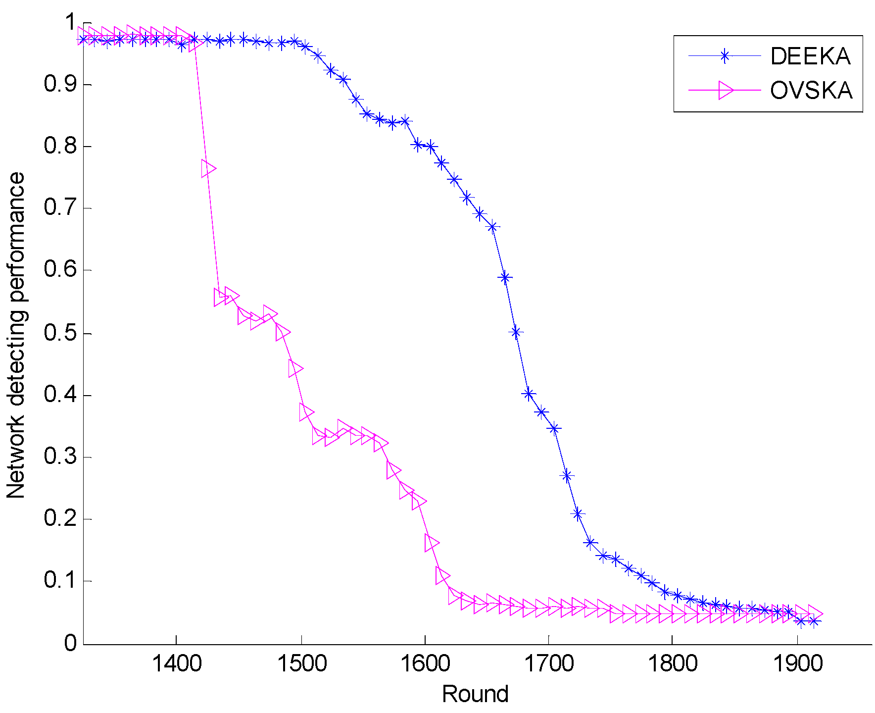
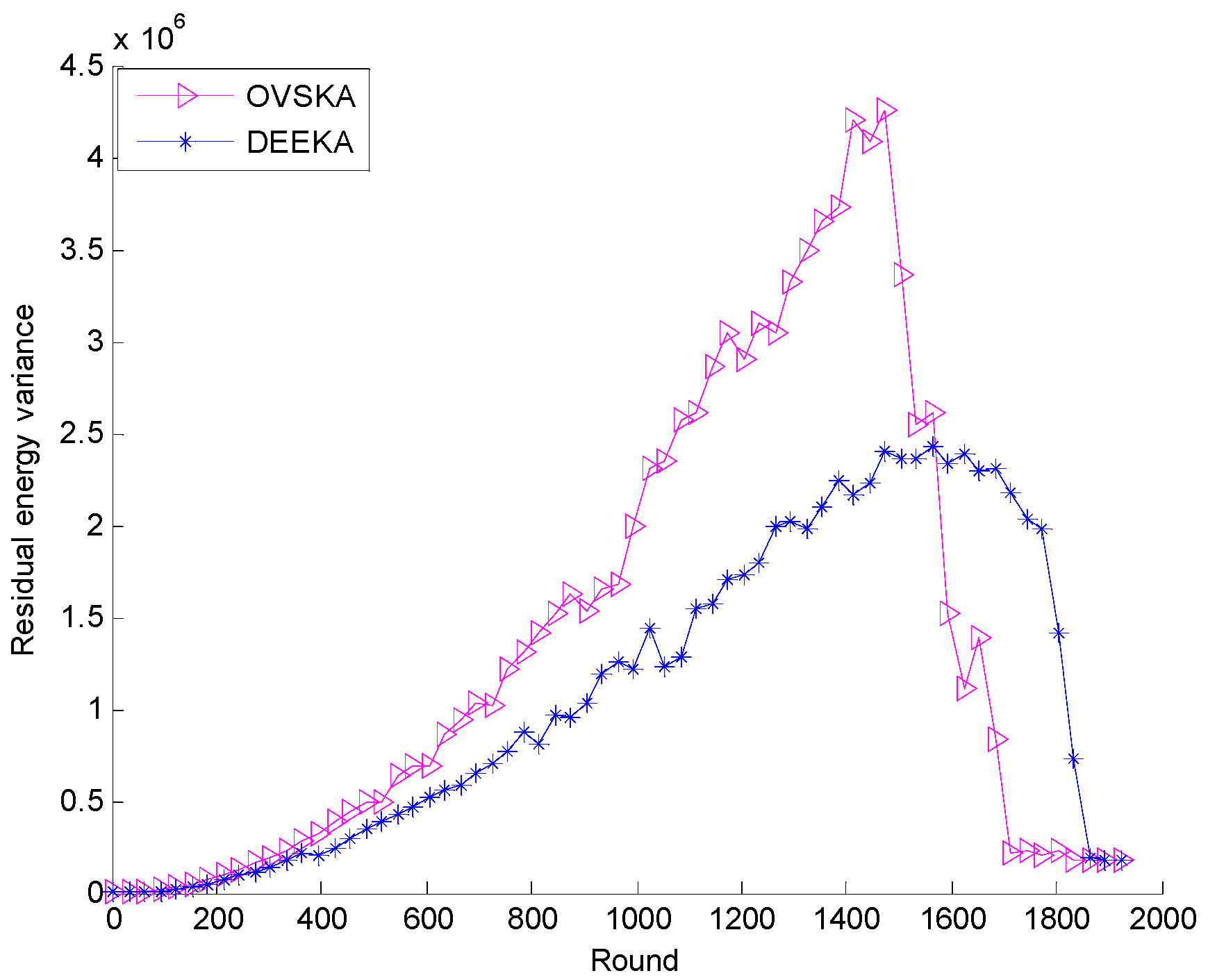
5.2.1. Comparison with the OVSKA
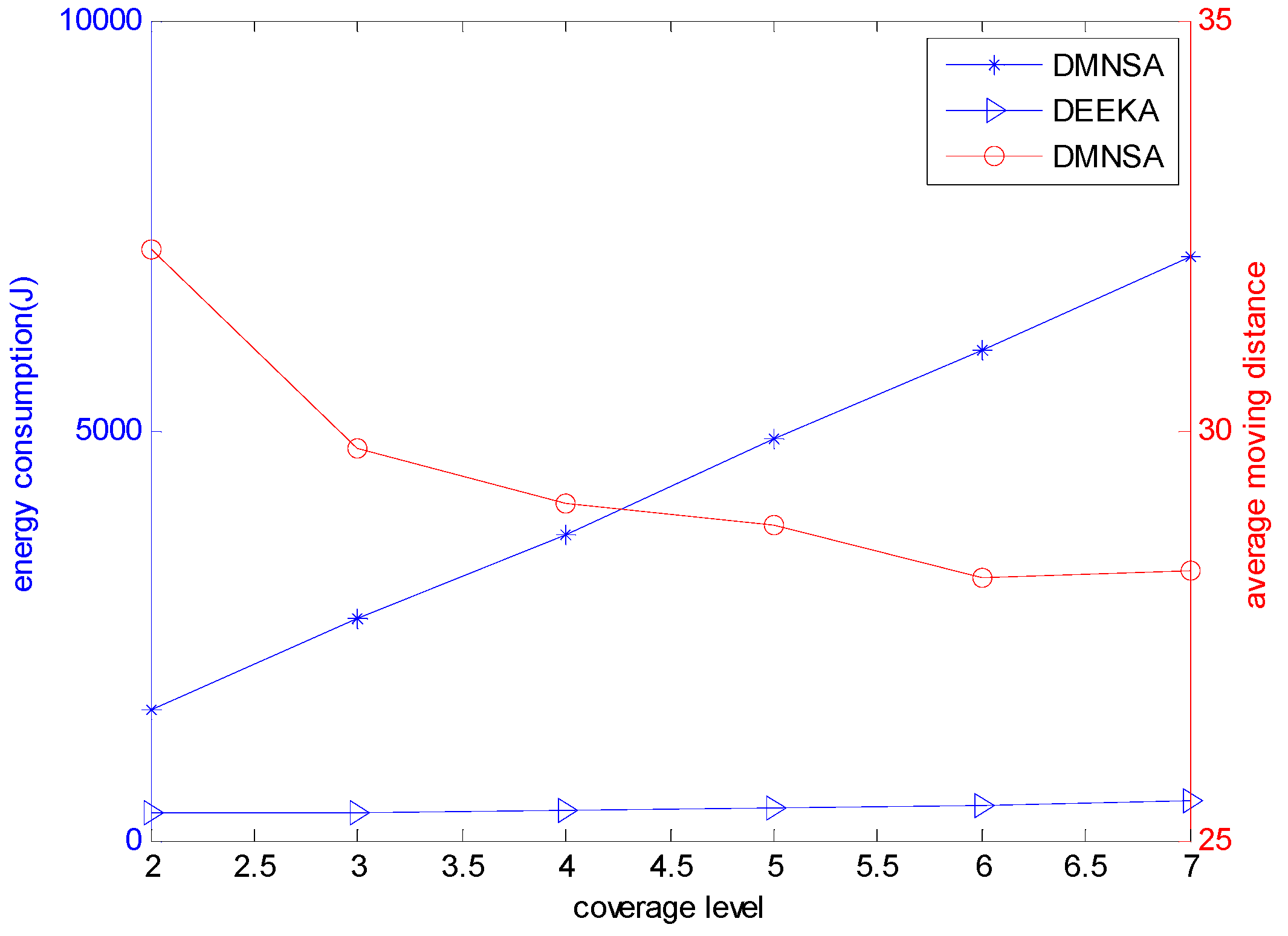
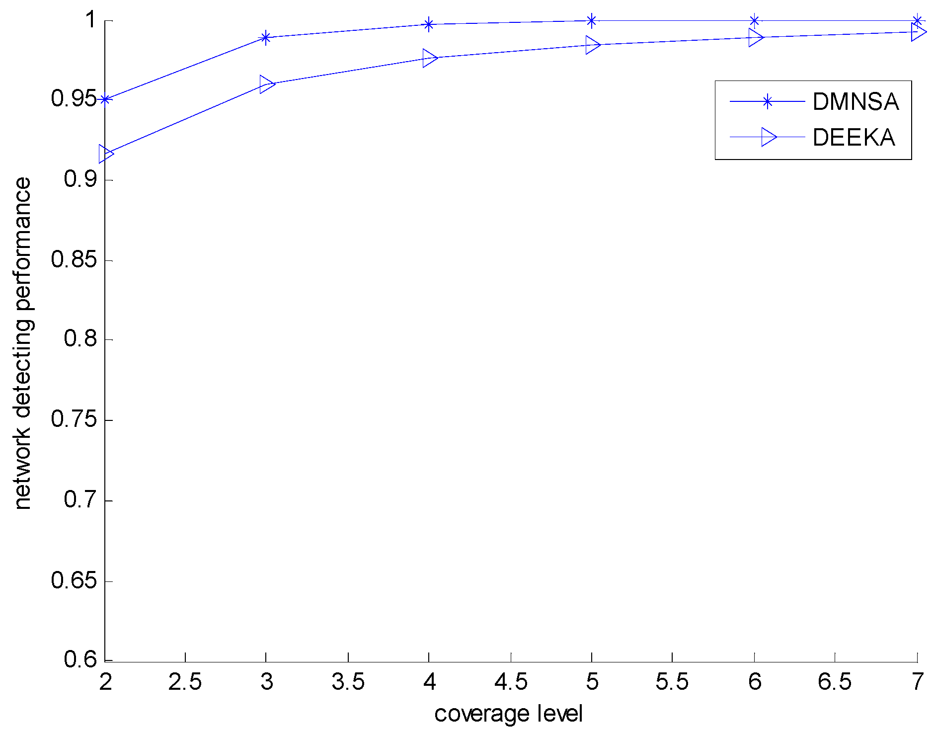
5.2.2. Comparison with the DMNSA
6. Conclusions
Acknowledgments
Author Contributions
Conflicts of Interest
References
- Guo, Z.W.; Luo, H.J.; Hong, F.; Yang, M.; Lionel, M.N. Current Progress and Research Issues in Underwater Sensor Networks. J. Comput. Res. Dev. 2010, 47, 377–389. [Google Scholar]
- Heidemann, J.; Stojanovic, M.; Zorzi, M. Underwater sensor networks: Applications, advances and challenges. Philos. Trans. R. Soc. Lond. A Math. Phys. Eng. Sci. 2012, 370, 158–175. [Google Scholar] [CrossRef] [PubMed]
- Lloret, J. Underwater sensor nodes and networks. Sensors 2013, 13, 11782–11796. [Google Scholar] [CrossRef] [PubMed]
- Yick, J.; Mukherjee, B.; Ghosal, D. Wireless sensor network survey. Comput. Netw. 2008, 52, 2292–2330. [Google Scholar] [CrossRef]
- Han, G.; Zhang, C.; Shu, L.; Sun, N.; Li, Q. A survey on deployment algorithms in underwater acoustic sensor networks. Int. J. Distrib. Sens. Netw. 2013, 1, 1–11. [Google Scholar] [CrossRef]
- Sendra, S.; Lloret, J.; García, M. Power saving and energy optimization techniques for wireless sensor neworks. J. Commun. 2011, 6, 439–459. [Google Scholar] [CrossRef]
- Ye, W.; Heidemann, J.; Estrin, D. An energy-efficient MAC protocol for wireless sensor networks. In Proceedings of the Twenty-First Annual Joint Conference of the IEEE Computer and Communications Societies, INFOCOM, New York, NY, USA, 23–27 June 2002; pp. 1567–1576.
- Ganesan, D.; Govindan, R.; Shenker, S.; Estrin, D. Highly-resilient, energy-efficient multipath routing in wireless sensor networks. ACM SIGMOBILE Mob. Comput. Commun. Rev. 2001, 5, 11–25. [Google Scholar] [CrossRef]
- Chen, G.; Li, C.; Ye, M. An unequal cluster-based routing protocol in wireless sensor networks. Wirel. Netw. 2009, 15, 193–207. [Google Scholar] [CrossRef]
- Garcia, M.; Sendra, S.; Lloret, J.; Murshed, M. Saving energy and improving communications using cooperative group-based wireless sensor networks. Telecommun. Syst. 2013, 52, 2489–2502. [Google Scholar] [CrossRef]
- Alam, K.M.; Kamruzzaman, J.; Karmakar, G.; Murshed, M.; Azad, A.K.M. QoS support in event detection in WSN through optimal k-coverage. Procedia Comput. Sci. 2011, 4, 499–507. [Google Scholar] [CrossRef]
- Zhou, Z.; Das, S.; Gupta, H. Connected k-coverage problem in sensor networks. In Proceedings of the 13th International Conference on Computer Communications and Networks, ICCCN 2004, Chicago, IL, USA, 11–13 October 2004; pp. 373–378.
- Li, L.; Zhang, B.; Zheng, J. A study on one-dimensional k-coverage problem in wireless sensor networks. Wirel. Commun. Mob. Comput. 2013, 13, 1–11. [Google Scholar] [CrossRef]
- Ammari, H.M.; Das, S.K. A study of k-coverage and measures of connectivity in 3D wireless sensor networks. IEEE Trans. Comput. 2010, 59, 243–257. [Google Scholar] [CrossRef]
- Ammari, H.M. A unified framework for k-coverage and data collection in heterogeneous wireless sensor networks. J. Parallel Distrib. Comput. 2016, 89, 37–49. [Google Scholar] [CrossRef]
- Ammari, H.M. 3D-k Cov-ComFor: An Energy-Efficient Framework for Composite Forwarding in Three-Dimensional Duty-Cycled k-Covered Wireless Sensor Networks. ACM Trans. Sens. Netw. 2016, 12, 35. [Google Scholar] [CrossRef]
- Kumar, S.; Lai, T.H.; Balogh, J. On k-coverage in a mostly sleeping sensor network. In Proceedings of the 10th Annual International Conference on Mobile Computing and Networking, Philadelphia, PA, USA, 26 September–1 October 2004; ACM: New York, NY, USA, 2004; pp. 144–158. [Google Scholar]
- Jiang, P.; Ruan, B.F. Cluster-Based Coverage-Preserving Routing Algorithm for Underwater Sensor Networks. Acta Electron. Sin. 2013, 10, 2067–2073. [Google Scholar]
- Kim, H.; Kim, E.J.; Yum, K.H. ROAL: A randomly ordered activation and layering protocol for ensuring K-coverage in wireless sensor networks. In Proceedings of the Third International Conference on Wireless and Mobile Communications, Guadeloupe, French, 4–9 March 2007; p. 4.
- Ammari, H.M. On the problem of k-coverage in 3D wireless sensor networks: A Reuleaux tetrahedron-based approach. In Proceedings of the 2011 Seventh International Conference on Intelligent Sensors, Sensor Networks and Information Processing (ISSNIP), Adelaide, Australia, 6–9 December 2011; pp. 389–394.
- Gupta, H.; Rao, S.; Venkatesh, T. Sleep Scheduling Protocol for k-Coverage of Three-Dimensional Heterogeneous WSNs. IEEE Trans. Veh. Technol. 2015, 65, 8423–8431. [Google Scholar] [CrossRef]
- Pal, M.; Medhi, N. Sixsoid: A new paradigm for k-coverage in 3D wireless sensor networks. In Proceedings of the 2015 International Conference on Computing, Communication and Security (ICCCS), Pamplemousses, Mauritius, 4–5 December 2015; pp. 1–5.
- Zeng, D.; Wu, X.; Wang, Y. A Survey on Sensor Deployment in Underwater Sensor Networks. Advances in Wireless Sensor Networks; Springer: Berlin/Heidelberg, Germany, 2014; pp. 133–143. [Google Scholar]
- Liu, B.; Dousse, O.; Nain, P.; Towsley, D. Dynamic Coverage of Mobile Sensor Networks. IEEE Trans. Parallel Distrib. Syst. 2013, 24, 301–311. [Google Scholar] [CrossRef]
- Chen, Z.; Gao, X.; Wu, F.; Chen, G. A PTAS to minimize mobile sensor movement for target coverage problem. In Proceedings of the INFOCOM 2016—The 35th Annual IEEE International Conference on Computer Communications, San Francisco, CA, USA, 10–14 April 2016; pp. 1–9.
- Ammari, H.M. On the problem of k-coverage in mission-oriented mobile wireless sensor networks. Comput. Netw. 2012, 56, 1935–1950. [Google Scholar] [CrossRef]
- Xia, N.; Wang, C.S.; Zheng, R. Fish swarm inspired underwater sensor deployment. Acta Autom. Sin. 2012, 38, 295–302. [Google Scholar] [CrossRef]
- Du, H.; Xia, N.; Zheng, R. Particle Swarm Inspired Underwater Sensor Self-Deployment. Sensors 2014, 14, 15262–15281. [Google Scholar] [CrossRef] [PubMed]
- Detweiler, C.; Doniec, M.; Vasilescu, I.; Rus, D. Autonomous Depth Adjustment for Underwater Sensor Networks: Design and Applications. IEEE/ASME Trans. Mechatron. 2012, 17, 16–24. [Google Scholar] [CrossRef]
- Alam, K.M.; Kamruzzaman, J.; Karmakar, G.; Murshed, M. Dynamic adjustment of sensing range for event coverage in wireless sensor networks. J. Netw. Comput. Appl. 2014, 46, 139–153. [Google Scholar] [CrossRef]
- Han, G.; Zhang, C.; Shu, L.; Rodrigues, J.J.P.C. Impacts of deployment strategies on localization performance in underwater acoustic sensor networks. IEEE Trans. Ind. Electron. 2015, 62, 1725–1733. [Google Scholar] [CrossRef]
- Zhou, Z.; Das, S.R.; Gupta, H. Variable radii connected sensor cover in sensor networks. ACM Trans. Sens. Netw. 2009, 5, 8–19. [Google Scholar] [CrossRef]
- Ahmed, S.; Javaid, N.; Khan, F.A.; Durrani, M.Y.; Ali, A.; Shaukat, A.; Sandhu, M.M.; Khan, Z.A.; Qasim, Q. Co-UWSN: Cooperative Energy-Efficient Protocol for Underwater WSNs. Int. J. Distrib. Sens. Netw. 2015, 75, 59–72. [Google Scholar] [CrossRef] [PubMed]
- Dantu, K.; Rahimi, M.; Shah, H.; Babel, H.; Dhariwal, A. Robomote: Enabling mobility in sensor networks. In Proceedings of the 4th International Symposium on Information Processing in Sensor Networks, Los Angeles, CA, USA, 24–27 April 2005; IEEE Press: Piscataway, NJ, USA, 2005. [Google Scholar]
- Elfes, A. Occupancy grids: A stochastic spatial representation for active robot perception. arXiv, 2013; arXiv:1304.1098. [Google Scholar]
- Bahi, J.; Haddad, M.; Hakem, M.; Kheddouci, H. Efficient distributed lifetime optimization algorithm for sensor networks. Ad Hoc Netw. 2014, 16, 1–12. [Google Scholar] [CrossRef]
- Liangqing, L.; Mengjue, L. Statistics, 2nd ed.; Hunan University Press: Changsha, China, 2014; pp. 132–149. [Google Scholar]
- Deb, K.; Pratap, A.; Agarwal, S.; Meyarivan, T. A fast and elitist multiobjective genetic algorithm: NSGA-II. IEEE Trans. Evol. Comput. 2002, 6, 182–197. [Google Scholar] [CrossRef]
- Jia, J.; Chen, J.; Chang, G.; Wen, Y.; Song, J. Multi-objective optimization for coverage control in wireless sensor network with adjustable sensing radius. Comput. Math. Appl. 2009, 57, 1767–1775. [Google Scholar] [CrossRef]
- Huang, J.; Wang, Z.; Ma, R. A New Genetic Algorithm for Constrained Multi-objective Optimization Problems. Comput. Eng. Appl. 2006, 42, 47–51. [Google Scholar]
- Zhou, J.; Li, J.; Zhang, Y. Efficient deployment scheme selection based on TOPSIS for clustering protocols of WSN. J. Netw. 2014, 9, 1838–1845. [Google Scholar] [CrossRef]


| Parameter | Value | Parameter | Value |
|---|---|---|---|
| Information transmission failure plost | 0.2 | Minimum sensing radius | 10 m |
| Energy consumption of data reception Pr | 5 mW | Maximum sensing radius | 28 m |
| Data transmission speed underwater | 1000 bit/s | Communication radius Rc | 20 m |
| Interval of algorithm operation T | 6 s | Length of data packet l | 150 bit |
| Adjusting parameters | 0.23, 0.71 | Energy diffusion factor λ | 1.5 |
| k1, a | 1, 10 | Carrier frequency f | 24 kHZ |
| Ratio of sensing to communication power rp | 43/80 | Maximum iteration number | 300 |
| Values of weight w1,w2,w3 | 1/3, 1/3, 1/3 | Number of population np | 60 |
© 2017 by the authors; licensee MDPI, Basel, Switzerland. This article is an open access article distributed under the terms and conditions of the Creative Commons Attribution (CC-BY) license (http://creativecommons.org/licenses/by/4.0/).
Share and Cite
Jiang, P.; Xu, Y.; Liu, J. A Distributed and Energy-Efficient Algorithm for Event K-Coverage in Underwater Sensor Networks. Sensors 2017, 17, 186. https://doi.org/10.3390/s17010186
Jiang P, Xu Y, Liu J. A Distributed and Energy-Efficient Algorithm for Event K-Coverage in Underwater Sensor Networks. Sensors. 2017; 17(1):186. https://doi.org/10.3390/s17010186
Chicago/Turabian StyleJiang, Peng, Yiming Xu, and Jun Liu. 2017. "A Distributed and Energy-Efficient Algorithm for Event K-Coverage in Underwater Sensor Networks" Sensors 17, no. 1: 186. https://doi.org/10.3390/s17010186