
Compound Event Barrier Coverage in Wireless Sensor Networks under Multi-Constraint Conditions


Abstract
:1. Introduction
- The compound event barrier coverage problem is formulated based on a joint probability model. At the same time, the joint probabilistic model is used to solve the problem of effectively merging sub-event confidence in the barrier coverage problem. To the best of our knowledge, this is the first work to study the compound event barrier coverage optimization problem.
- The problem of compound event barrier coverage with time constraints, distance constraints, cost constraints and minimum confidence constraints is proposed. In battlefield applications, in order to take the preemptive actions, it is necessary to complete the barrier coverage within a limited time, so the barrier coverage problem is time-bound. At the same time, due to the complex terrain of the battlefield, such as the existence of rivers and minefields, the barrier coverage path will be limited. In battlefields and other hazardous environment, the logistics supply will be limited, so the barrier coverage will also be subject to cost constraints. In this paper, a multiplier method based on active-set strategy is proposed, which effectively solves the problem of compound event barrier coverage under time constraints, distance constraints, cost constraints and minimum confidence constraints, etc. To the best of our knowledge, this is the first work to study the compound event barrier coverage optimization problem under multiple constraints.
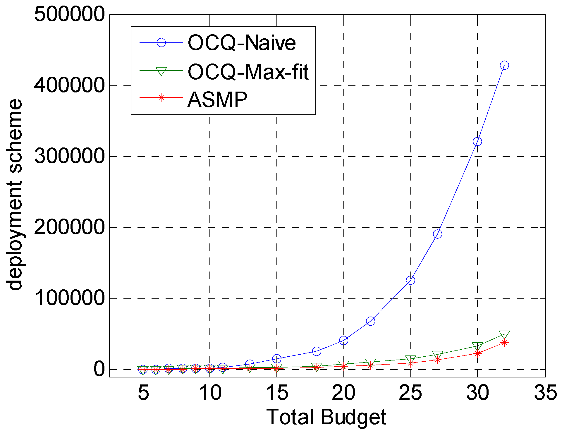
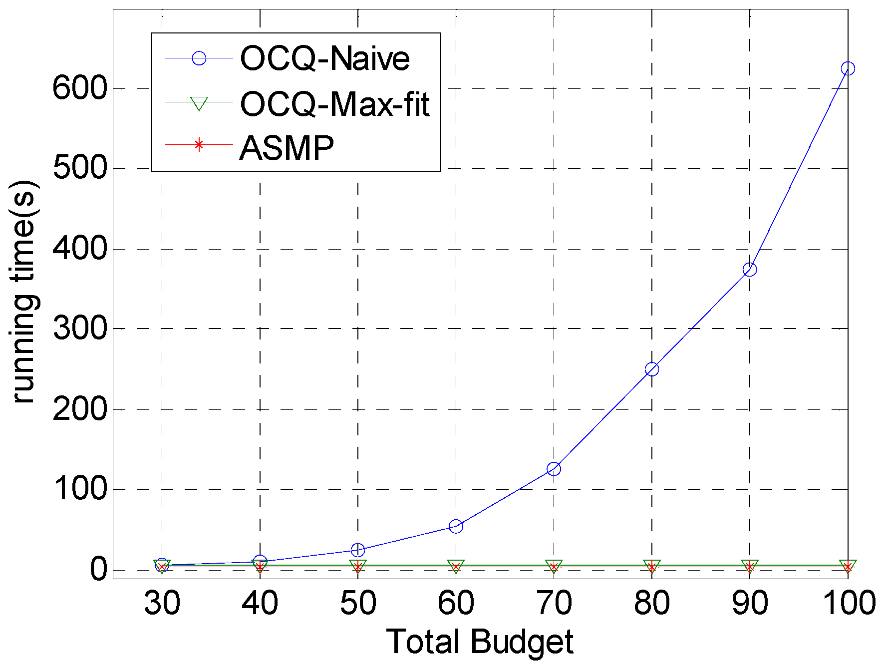
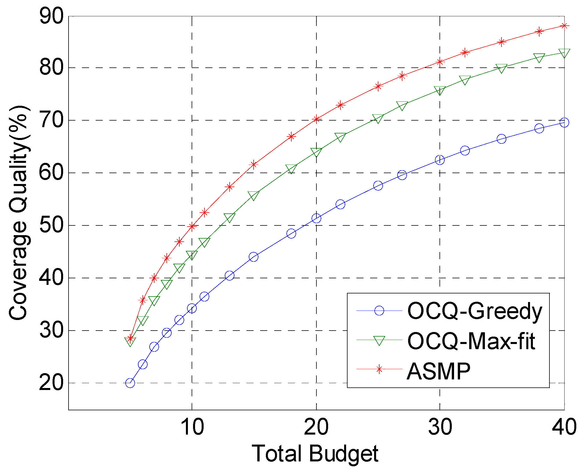
- The effectiveness and efficiency of our compound event barrier coverage mechanism are better than previous algorithms as proved by extensive simulations. The results show that our technique is more computationally efficient, especially when the network topology is relatively complex.
2. Related Works
3. The Event Model
4. Compound Event Barrier Coverage Optimization Problem
4.1. Main Idea
4.2. Problem Formulation
4.3. Active Set Multiplier Policy (ASMP)
| Algorithm 1: Sub-event Algorithm |
| 1: Initialization: |
| 2: Solve the equation set for . Determine the search direction . |
| 3: Determine the smallest non-negative integer for that satisfies the constraint: |
| 4: Do , ; |
| 5: Judge, if , make , then exit; Otherwise, set , Skip back to step 1. |
| Algorithm 2: Active Set Multiplier Policy (ASMP) |
| 1: Initialization: |
| 2: Set |
| 3: Solving sub-events: Utilizing as the initial point, use Algorithm 1 to solve the unconstrained problem to get the maximum point ; |
| 4: Verify termination conditions: If does not satisfied, skip to step 3; if , then stop; otherwise set , go to step 2; |
| 5: Update penalty parameters: If , set ; otherwise set ; |
| 6: Update multipliers: ; |
| 7: Set , skip to step 1. |
5. Experiments and Evaluation
5.1. Environment Settings
5.2. Experimental Evaluation
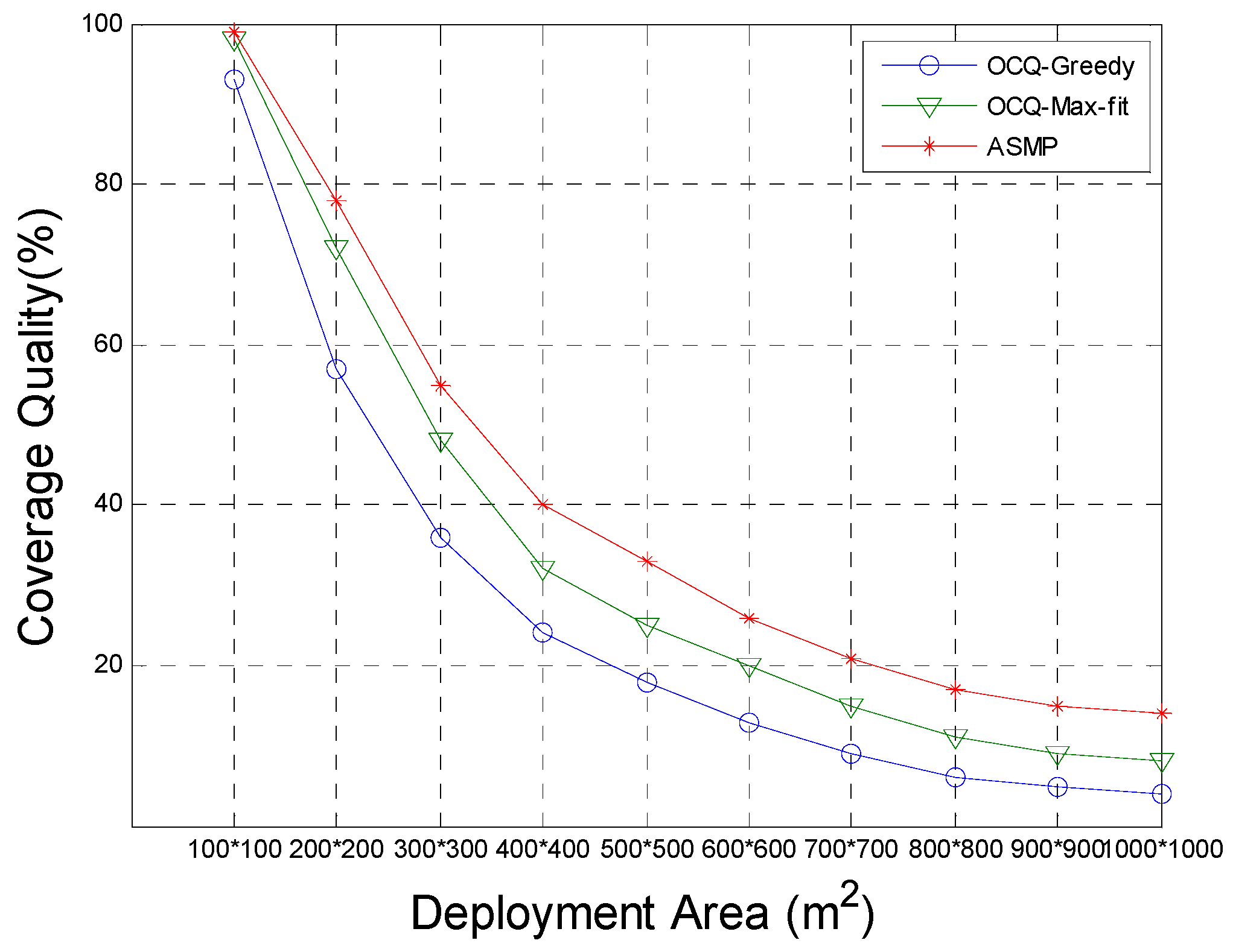
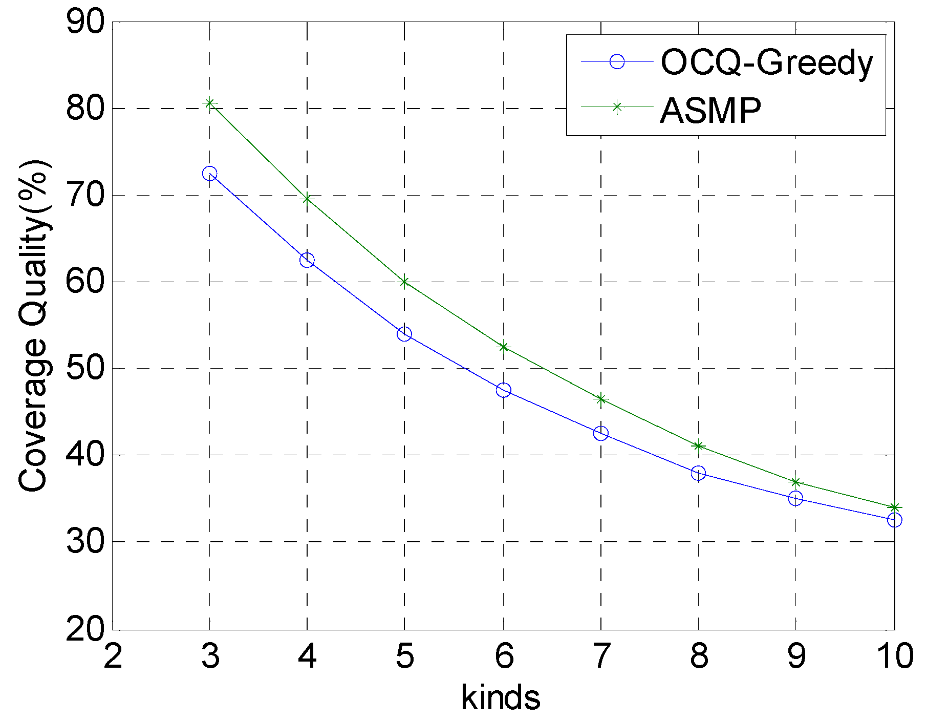
5.3. Comparison with the OCQ-Max-Fit, OCQ-Greedy and OCQ-Naïve Algorithms
6. Conclusions and Future Work
Acknowledgments
Author Contributions
Conflicts of Interest
References
- Tao, D.; Wu, T.Y. A Survey on Barrier Coverage Problem in Directional Sensor Networks. IEEE Sens. J. 2015, 152, 876–885. [Google Scholar]
- Chen, A.; Kumar, S. Local Barrier Coverage in Wireless Sensor Networks. IEEE Trans. Mob. Comput. 2010, 94, 491–504. [Google Scholar] [CrossRef]
- Tao, D.; Tang, S.J. Strong barrier coverage in directional sensor networks. Comput. Commun. 2012, 358, 895–905. [Google Scholar] [CrossRef]
- He, S.B.; Gong, X.W. Curve-Based Deployment for Barrier Coverage in Wireless Sensor Networks. IEEE Trans. Wirel. Commun. 2014, 132, 724–735. [Google Scholar] [CrossRef]
- Ma, H.; Yang, M.; Li, D.Y. Minimum camera barrier coverage in wireless camera sensor networks. In Proceedings of the IEEE INFOCOM, Orlando, FL, USA, 25–30 March 2012; pp. 217–225.
- Abhilash, C.N.; Manjula, S.H.; Venugopal, K.R. Efficient network lifetime for barrier coverage in heterogeneous sensor network. In Proceedings of the IEEE INDICON, IIT Bombay, Mumbai, India, 13–15 December 2013; pp. 1–4.
- Dewitt, J.; Shi, H.C. Maximizing lifetime for k-barrier coverage in energy harvesting wireless sensor networks. In Proceedings of the IEEE Global Communications Conference, Austin, TX, USA, 8–12 December 2014; pp. 300–304.
- Dewitt, J.; Patt, S.; Shi, H.C. Maximizing continuous barrier coverage in energy harvesting sensor networks. In Proceedings of the IEEE International Conference on Communications, Sydney, Australia, 10–14 June 2014; pp. 172–177.
- Gao, J.; Li, J.Z. Model-Based Approximate Event Detection in Heterogeneous Wireless Sensor Networks. In Wireless Algorithms, Systems, and Applications; Cai, Z.P., Wang, C.K., Eds.; Springer International Publishing: Cham, Switzerland, 2014; Volume 8491, pp. 225–235. [Google Scholar]
- Gao, J.; Li, J.Z.; Cai, Z.P. Composite event coverage in wireless sensor networks with heterogeneous sensors. In Proceedings of the IEEE INFOCOM, Hong Kong, China, 26 April–1 March 2015; pp. 217–225.
- Arivudainambi, D.; Balaji, S.; Deepika, S. Connected coverage in wireless sensor networks using genetic algorithm. In Proceedings of the IEEE Workshop on Computational Intelligence: Theories, Applications and Future Directions, Kanpur, India, 14–17 December 2015; pp. 1–6.
- Romoozi, M.; Vahidipour, M.; Romoozi, M. Genetic Algorithm for Energy Efficient and Coverage-Preserved Positioning in Wireless Sensor Networks. In Proceedings of the International Conference on Intelligent Computing and Cognitive Informatics, Kuala Lumpur, Malaysia, 22–23 June 2010; pp. 22–25.
- Zhang, K.; Zhang, W.; Jia, T.H. Genetic simulated annealing based coverage-enhancing algorithm for deployment of directional Doppler sensors system. In Proceedings of the International Workshop on Microwave and Millimeter Wave Circuits and System Technology, Chengdu, China, 19–20 April 2012; pp. 1–4.
- Chen, C. A Coverage Algorithm for WSN Based on the Improved PSO. In Proceedings of the International Conference on Intelligent Transportation, Halong Bay, Vietnam, 19–20 December 2015; pp. 12–15.
- Manjula, R.B.; Manvi, S.S. Coverage optimization based sensor deployment by using PSO for anti-submarine detection in UWASNs. In Proceedings of the Ocean Electronics, Kochi, India, 23–25 October 2013; pp. 15–22.
- Zhu, C.; Zheng, C. A survey on coverage and connectivity issues in wireless sensor networks. J. Netw. Comput. Appl. 2012, 352, 619–632. [Google Scholar] [CrossRef]
- Shan, A.; Xu, X.; Cheng, Z. Target Coverage in Wireless Sensor Networks with Probabilistic Sensors. Sensors 2016, 16, 1372. [Google Scholar] [CrossRef] [PubMed]
- Kilic, V.T.; Unal, E.; Demir, H.V. Wireless Metal Detection and Surface Coverage Sensing for All-Surface Induction Heating. Sensors 2016, 16, 363. [Google Scholar] [CrossRef] [PubMed]
- Shih, K.P.; Deng, D.J.; Chang, R.S. On Connected Target Coverage for Wireless Heterogeneous Sensor Networks with Multiple Sensing Units. Sensors 2009, 97, 5173–5200. [Google Scholar] [CrossRef] [PubMed]
- Li, J.; Andrew, L.L.; Foh, C.H. Connectivity, coverage and placement in wireless sensor networks. Sensors 2009, 9, 7664–7693. [Google Scholar] [CrossRef] [PubMed]
- Akbarzadeh, V.; Levesque, J.C.; Gagne, C. Efficient Sensor Placement Optimization Using Gradient Descent and Probabilistic Coverage. Sensors 2014, 148, 15525–15552. [Google Scholar] [CrossRef] [PubMed]
- Peng, J.; Shuai, L.; Liu, J. A Depth-Adjustment Deployment Algorithm Based on Two-Dimensional Convex Hull and Spanning Tree for Underwater Wireless Sensor Networks. Sensors 2016, 16, 1087. [Google Scholar] [CrossRef] [PubMed]
- Urdiales, C.; Aguilera, F.; Gonzálezparada, E. Rule-Based vs. Behavior-Based Self-Deployment for Mobile Wireless Sensor Networks. Sensors 2016, 16, 1047. [Google Scholar] [CrossRef] [PubMed]
- Zalyubovskiy, V.; Erzin, A.; Astrakov, S. Energy-efficient Area Coverage by Sensors with Adjustable Ranges. Sensors 2009, 94, 2446–2460. [Google Scholar] [CrossRef] [PubMed]
- Kumar, S.; Lai, T.H. Barrier coverage with wireless sensors. Wirel. Netw. 2007, 136, 817–834. [Google Scholar] [CrossRef]
- Chen, A.; Li, Z.; Lai, T.H. One-way barrier coverage with wireless sensors. In Proceedings of the IEEE INFOCOM, Shanghai, China, 10–15 April 2011; pp. 626–630.
- Tao, D.; Tang, S. Strong Barrier Coverage Detection and Mending Algorithm for Directional Sensor Networks. Ad Hoc Sens. Wirel. Netw. 2013, 181, 17–33. [Google Scholar]
- Luo, J.; Zou, S. Strong-Barrier Coverage for One-Way Intruders Detection in Wireless Sensor Networks. Int. J. Distrib. Sens. Netw. 2016, 2016, 3807824. [Google Scholar] [CrossRef]
- Lazos, L.; Poovendran, R. Coverage in Heterogeneous Sensor Networks. In Proceedings of the International Symposium on Modeling and Optimization in Mobile, Ad Hoc and Wireless Networks, Boston, MA, USA, 3–6 April 2006; pp. 1–10.
- Yu, J.; Chen, Y. On Connected Target k-Coverage in Heterogeneous Wireless Sensor Networks. Sensors 2016, 161, 262–265. [Google Scholar] [CrossRef] [PubMed]
- Tian, J.; Liang, X. Deployment and reallocation in mobile survivability-heterogeneous wireless sensor networks for barrier coverage. Ad Hoc Netw. 2015, 36, 321–331. [Google Scholar] [CrossRef]
- Yang, Y.; Ambrose, A. Coverage for composite event detection in wireless sensor networks. Wirel. Commun. Mob. Comput. 2011, 118, 1168–1181. [Google Scholar] [CrossRef]
- Zhou, Z.; Xing, R. Event Coverage Detection and Event Source Determination in Underwater Wireless Sensor Networks. Sensors 2015, 1512, 31620–31643. [Google Scholar] [CrossRef] [PubMed]
- Chen, Z.; Li, S. Memetic algorithm-based multi-objective coverage optimization for wireless sensor networks. Sensors 2014, 1411, 20500–20518. [Google Scholar] [CrossRef] [PubMed]
- Prasan, K.S.; Ming-Jer, C. An Efficient Distributed Coverage Hole Detection Protocol for Wireless Sensor Networks. Sensors 2016, 16, 386. [Google Scholar] [CrossRef] [PubMed]
- Cheng, C.T.; Leung, H. Performance evaluation of transmission power optimization formulations in wireless sensor networks using pareto optimality. In Proceedings of the IEEE International Conference on Systems, Man, and Cybernetics, Seoul, Korea, 14–17 October 2012; pp. 1257–1261.
- Azad, P.; Sharma, V. Pareto-optimal clustering scheme using data aggregation for wireless sensor networks. Int. J. Electron. 2014, 1027, 1165–1176. [Google Scholar] [CrossRef]
- Leinonen, M.; Codreanu, M. Distributed Joint Resource and Routing Optimization in Wireless Sensor Networks via Alternating Direction Method of Multipliers. IEEE Trans. Wirel. Commun. 2013, 1211, 5454–5467. [Google Scholar] [CrossRef]
- Li, X.S. An Aggregate Function Method for Nonlinear Programming. Sci. China Ser. A 1991, 3412, 1467–1473. [Google Scholar] [CrossRef]
- Polak, E.; Womersley, R.S. An Algorithm Based on Active Sets and Smoothing for Discretized Semi-Infinite Minimax Problems. J. Optim. Theory Appl. 2008, 138, 311–328. [Google Scholar] [CrossRef]


| Symbol | Meaning | Deployment Time T/s | Perceived Radius R/m | Cost C/s | Confidence S |
|---|---|---|---|---|---|
| Optical Density Sensor | 1 | 30 | 25 | 0.1 | |
| Temperature Sensor | 2 | 15 | 10 | 0.05 | |
| Video Sensor | 5 | 10 | 35 | 0.45 | |
| Smoke Density Sensor | 1 | 25 | 20 | 0.15 | |
| Infrared Sensor | 3 | 20 | 15 | 0.25 |
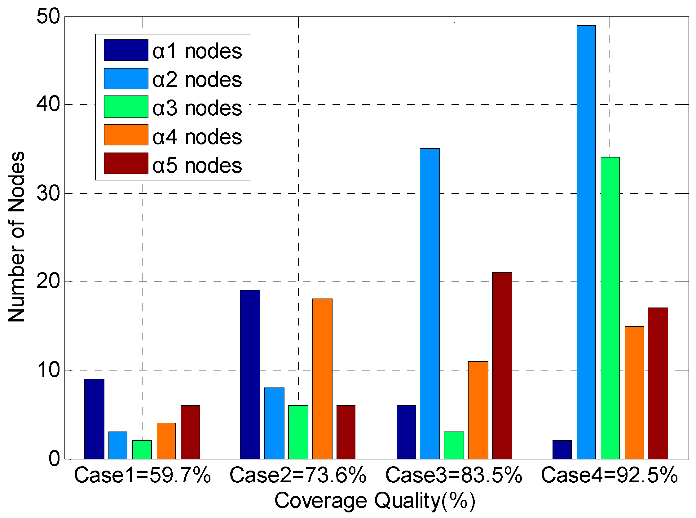
| Case | Time Constraints | Distance Constraints | Cost Constraints | Minimum Confidences | Coverage Ratio | Running Time |
|---|---|---|---|---|---|---|
| 1 | 47 | 555 | 495 | 0.80 | 59.7% | <1 s |
| 2 | 101 | 1320 | 1215 | 0.82 | 73.6% | <1 s |
| 3 | 165 | 1430 | 1140 | 0.90 | 83.5% | <1 s |
| 4 | 336 | 1850 | 2285 | 0.99 | 92.5% | <1 s |
© 2016 by the authors; licensee MDPI, Basel, Switzerland. This article is an open access article distributed under the terms and conditions of the Creative Commons Attribution (CC-BY) license (http://creativecommons.org/licenses/by/4.0/).
Share and Cite
Zhuang, Y.; Wu, C.; Zhang, Y.; Jia, Z. Compound Event Barrier Coverage in Wireless Sensor Networks under Multi-Constraint Conditions. Sensors 2017, 17, 25. https://doi.org/10.3390/s17010025
Zhuang Y, Wu C, Zhang Y, Jia Z. Compound Event Barrier Coverage in Wireless Sensor Networks under Multi-Constraint Conditions. Sensors. 2017; 17(1):25. https://doi.org/10.3390/s17010025
Chicago/Turabian StyleZhuang, Yaoming, Chengdong Wu, Yunzhou Zhang, and Zixi Jia. 2017. "Compound Event Barrier Coverage in Wireless Sensor Networks under Multi-Constraint Conditions" Sensors 17, no. 1: 25. https://doi.org/10.3390/s17010025