Node Redeployment Algorithm Based on Stratified Connected Tree for Underwater Sensor Networks

Abstract

During the underwater sensor networks (UWSNs) operation, node drift with water environment causes network topology changes. Periodic node location examination and adjustment are needed to maintain good network monitoring quality as long as possible. In this paper, a node redeployment algorithm based on stratified connected tree for UWSNs is proposed. At every network adjustment moment, self-examination and adjustment on node locations are performed firstly. If a node is outside the monitored space, it returns to the last location recorded in its memory along straight line. Later, the network topology is stratified into a connected tree that takes the sink node as the root node by broadcasting ready information level by level, which can improve the network connectivity rate. Finally, with synthetically considering network coverage and connectivity rates, and node movement distance, the sink node performs centralized optimization on locations of leaf nodes in the stratified connected tree. Simulation results show that the proposed redeployment algorithm can not only keep the number of nodes in the monitored space as much as possible and maintain good network coverage and connectivity rates during network operation, but also reduce node movement distance during node redeployment and prolong the network lifetime.

1. Introduction and Related Works

With rapid advances in technologies such as sensors, micro-electro-mechanical-systems (MEMS), wireless communication and embedded systems, wireless sensor networks (WSNs) have been widely used in applications like environment monitoring, military surveillance, industry or agriculture production, traffic control and heath care [1,2]. As application extension of conventional terrestrial WSNs, underwater sensor networks (UWSNs) are an kind of underwater monitoring system composed of nodes that are capable of information perception, data processing and communication, which also have such characteristics as using acoustic signal as communication medium, 3D network structure, limited and difficult-to-supplement node energy, node drift with water environment and relatively sparse node deployment density. Because of suitability for information acquisition in 3D underwater space, UWSNs have been widely used for seabed resources exploration, underwater pollution monitoring, and marine military [3,4,5]. Due to increasing attentions of many countries on marine resources, UWSNs have also become the research hotspot of current sensor network field. The UWSNs researches mainly involve node deployment [6,7,8], time synchronization [9,10], node localization [11,12], network route [13,14], energy balance and efficiency [15,16], etc. Among them, node deployment is not only closely related to network monitoring quality, but it is also the basis of other network protocol and algorithm designs [17].

There are many researches concerning UWSNs node deployment. According to different assumptions on node mobility, UWSNs node deployment algorithms can be classified into static, limited mobility and free mobility deployment [18]. The static deployment algorithm assumes that nodes are immovable and fixed at specific locations manually. Pompili et al. [19] proposed 2D and 3D UWSNs structures, and performed a deep mathematical analysis on node deployment on the basis of these two structures. Besides, they studied network robustness to node failures, and provided an estimate of the number of redundant sensors required. To realize full network coverage with the least nodes, Alam et al. [20] compared filling effect of truncated octahedron, cube, hexagonal prism and rhombic dodecahedron by using the idea of 3D Voronoi polyhedron tessellation. They found that truncated octahedron filling was the best strategy. Static node deployment algorithm can gain high network coverage and connectivity rates, and even realizes full network coverage and connectivity. However, it needed too large number of nodes and is not suitable for the sparse UWSNs deployment characteristic. Limited mobility node deployment algorithm assumes that nodes can only move vertically. Akkaya et al. [21] proposed a distributed self-organized node deployment algorithm, which reduced overlapped coverage by adopting the graph coloring idea. Nevertheless, this algorithm only emphasized on increasing network coverage rate and neglected network connectivity rate improvement. Hence, Senel et al. [22] put forward another distributed self-organized node deployment algorithm. It introduced in the connected dominating set (CDS) idea and maximized the network coverage rate under the premise of full network connectivity. Free mobility node deployment algorithm assumes that nodes can move toward all directions. Li et al. [23] proposed a 3D virtual forces deployment (TVFD) algorithm. It extended the 2D virtual forces deployment algorithm [24] to 3D space and was applicable to 3D underwater environment. Although it could improve network coverage and connectivity rates, it could not ensure full network connectivity (i.e., the network connectivity rate was 1). Besides, the network coverage rate could still be improved significantly. To realize effective coverage on events in the monitored underwater space, after proposing the fish-inspired node deployment algorithm [25], Xia et al. further put forward the similar particle swarm inspired node deployment (PSIND) algorithm [26]. This kind of algorithm made full use of behavioral features of fish or particle swarm, and was able to drive nodes to cover events as many as possible in the monitored underwater space.

As a research team which has been keeping much focus on WSNs, we have also proposed many node deployment algorithms for UWSNs in recent years [27,28,29,30,31]. A depth adjustment node self-deployment algorithm was proposed in reference [27], the main purpose of which was to improve the network connectivity rate achieved by the algorithm proposed in reference [21] and save network energy consumption caused by the algorithm proposed in reference [22]. An uneven cluster and radius-adjusting self-deployment algorithm was proposed in reference [28], the main purpose of which was to improve network reliability and balance energy consumption during network operation ignored by the algorithm proposed in reference [22]. These two algorithms belonged to limited mobility deployment, while the algorithm proposed in the following of this paper belonged to free mobility deployment, which also included our works proposed in references [29,30,31]. The work in reference [29] mainly focused on the node location determination and dispatch problem, the former was solved by the greedy iterative strategy where the connectivity nodes were used to improve the network connectivity rate until the full network connectivity was achieved and the latter was solved by the Kuhn-Munkres algorithm with the help of command nodes. The work in reference [30] proposed a node deployment algorithm based on CDS (DBCDS) algorithm to optimize the same network performances with that in reference [29]. However, different with that in reference [29], the network topology formed after the DBCDS algorithm operation has relationship with the initial random node scattering on the water surface. The node non-uniform deployment based on clustering (NNDBC) algorithm for UWSNs was proposed in reference [31], in which a high network connectivity rate was achieved by determining the heterogeneous communication ranges of nodes during node clustering, and the nodes with lower aggregate contribution degrees were used to substitute the dying nodes to decrease the total movement distance of nodes and prolong the network lifetime. The main difference between the NNDBC algorithm and our other works in references [27,28,29,30] as well as this paper was that the coverage targets in the NNDBC algorithm were isolated events, whose distributions were usually non-uniform in the monitored space.

In other words, those above researches did not fully consider node drift caused by water environment during network operation. Actually, if this is considered fully, the UWSNs node deployment problem can be converted into the UWSNs node redeployment problem. For study convenience, this paper defines the UWSNs node redeployment problem as periodic examination and adjustment on node locations with full consideration of the UWSNs characteristics (especially node drift with water environment during network operation). The main optimizing aim of this problem is to improve the network coverage and connectivity rates during network operation, reduce energy consumption during node redeployment as much as possible, and prolong the network lifetime as long as possible. Few researches on the UWSNs redeployment problem have been reported yet. Liu et al. [32] described the node drift with water environment during network operation with the 3D random drift model, and put forward the moving redundancy nodes redeployment (MRNR) algorithm. At every network adjustment moment, the sink node repeatedly requires the least important node, which makes the smallest contribution to the network coverage rate, to move toward the biggest coverage blind point. This could result in large network coverage rate improvement, but failed to keep nodes in the monitored underwater space effectively and did not consider how to improve the network connectivity during network operation. Moreover, this algorithm did not optimize the movement distance of the least important node during node redeployment. Due to limited node energy and huge energy consumption for node movement in underwater environment, nodes may die quickly upon running out of energy, which shortens the network lifetime.

There are only few UWSNs node redeployment algorithms, and they are difficult to improve or maintain the network coverage and connectivity rates as long as possible with the probably least energy consumption while taking full consideration of node drift with water environment. Therefore, this paper put forward a node redeployment based on stratified connected tree (NRBSCT) algorithm. In every network adjustment moment, self-examination and adjustment on node locations are performed firstly. If a node finds that it is outside the monitored space, it returned to the last location recorded in its memory along the straight line, which helps to maintain the network monitoring quality. Later, the network is stratified, and the whole network topology is changed into a connected tree that takes the sink node as the root node by broadcasting ready information level by level, which can improve the network connectivity during network operation. Finally, synthetically considering the network coverage and connectivity rates, together with the node movement distance, the sink node performs centralized optimization on locations of leaf nodes in the stratified connected tree. Simulation results show that the proposed redeployment algorithm can not only keep the number of nodes in the monitored space as much as possible, maintain good network coverage and connectivity rates during network operation, but also reduce node movement distance during node redeployment and prolong the network lifetime.

Compared with the existing related algorithms, the contributions of the proposed NRBSCT algorithm are as follows:

(1)

It takes full consideration of node drift with water environment during network operation. At every network adjustment moment, nodes can keep themselves in the monitored space through self-examination and adjustment, which helps to maintain good network monitoring quality.

(2)

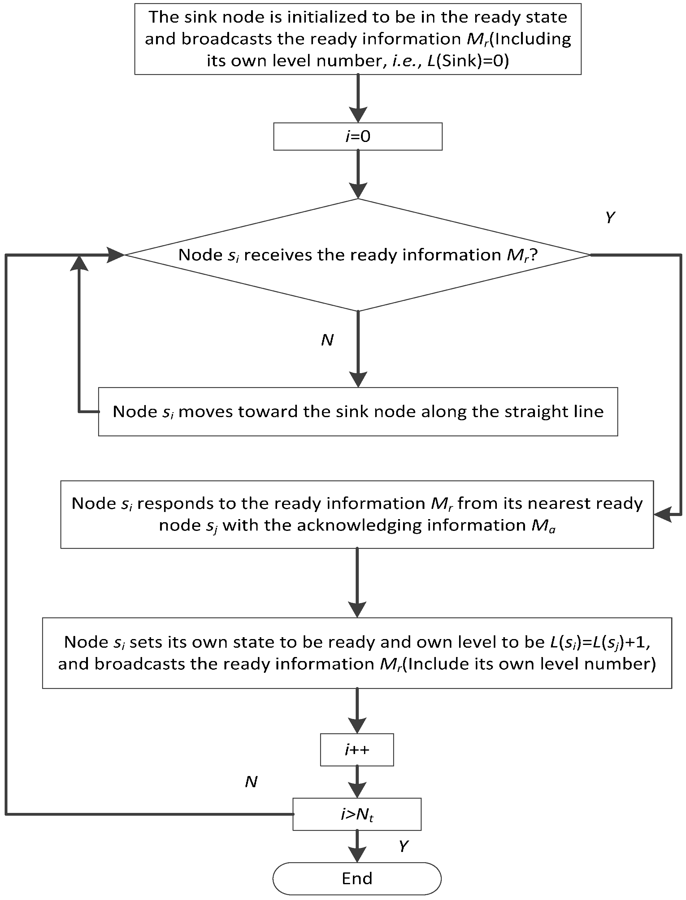
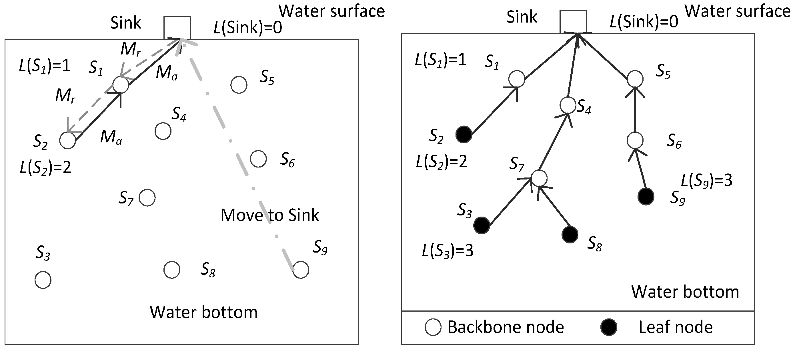
At every network adjustment moment, the network is converted into a stratified connected tree through level-by-level stratifying, which can achieve full network connectivity and lower the network connectivity decrease speed during network operation.

(3)

The sink node performs centralized optimization adjustment on the locations of leaf nodes in the stratified connected tree with synthetically considering the network coverage and connectivity rates, and node movement distance. This can not only maintain excellent network monitoring performances, but also reduce node movement distance during node redeployment, as well as prolong the network lifetime.

Table 1. Differences between the related research works and NRBSCT algorithm.

Literature/Algorithm	Node Mobility	Consideration of Node Drift with Water Environment
[19,20]	Static	No
[21,22,27]	limited	Additional
[28]	limited	No
[23,25,29,30,31]	Free	No
[26]	Free	Additional
[32], NRBSCT	Free	Full

is used to give a better description of the differences between the related research works and NRBSCT algorithm. The rest of the paper is organized as follows. In Section 2, the models, definitions and preliminaries involved in the NRBSCT algorithm are formally introduced. In Section 3, we elaborate the UWSNs node redeployment problem and corresponding NRBSCT algorithm. The simulation evaluation is provided in Section 4 with our conclusion and future work in Section 5.

2. Model, Definitions and Preliminaries

2.1. Models

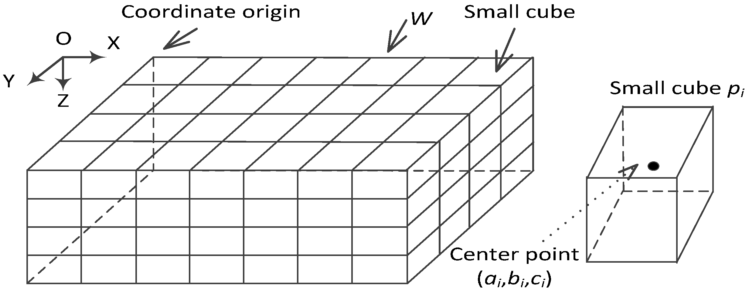
2.1.1. 3D Underwater Space Model

As is shown in Figure 1, the 3D underwater space is a large cube [33] divided into a number of small cubes whose side lengths are w. All the small cubes have selected their center points to represent themselves. The coordinates of cube p_i is (a_i,b_i,c_i).

2.1.2. Node Energy Consumption Model

Considering that the energy consumption of nodes for sensing, processing, and receiving information is much smaller than for transmitting information and moving [34], only the latter is considered. The energy consumption for transmitting information is modeled based on the method mentioned in reference [35]. According to the related content in reference [35], the specific method to calculate the energy consumption for transmitting information can be elaborated as follows. Supposing that d denotes the geometrical transmitting distance of the information package, which includes the necessary information used in the network redeployment process, such as the ID number, location and left energy of the node, and the size of the information package is denoted as M_b. T_p denotes the transmitting time of the information package and S_v is the transmission speed of the information package. On the one hand, we can calculate the transmitting time of the information package by the following formula:

$$T_p=\frac{M_b}{S_v}$$

(1)

On the other hand, the relationship between the frequency f (KHZ) of the carrier acoustic signal and the water absorption coefficient α(f) (dB/m) is calculated by the following formula:

$$\alpha \left(f\right)=0.11\frac{{10}^{-3}{f}^2}{1+f^2}+44\frac{{10}^{-3}{f}^2}{4100+f^2}+2.75\times {10}^{-7}{f}^2+3\times {10}^{-6}$$

(2)

When the transmitting distance of the information package is d, the energy attenuation is denoted as A(d) and can be calculated by the following formula:

$$\{\begin{array}{l}A\left(d\right)=d^{\lambda }\times {\beta }^d\\ \beta ={10}^{\alpha \left(f\right)/10}\end{array}$$

(3)

where λ is the energy spreading factor (λ is 1 for cylindrical, 1.5 for practical, and 2 for spherical spreading). Therefore, the energy consumption for transmitting information can be denoted as E_tx(d) and calculated by the following formula:

$$E_{tx}\left(d\right)=P_r\times T_p\times A\left(d\right)$$

(4)

where P_r denotes the power threshold for a node to receive the information package. Moreover, supposing that the number of information package transmitting times for node s in the network redeployment process is t_n, and the communication range for node s is R_t, the communication energy consumption C_e can be obtained by the following formula:

$$C_e=E_{tx}\left(R_t\right)*t_n$$

(5)

The movement energy consumption M_e can be defined as the product of the movement distance m_d and the energy consumption per movement distance m_u, which can be also described as follows:

$$M_e=m_d*m_u$$

(6)

2.1.3. Node Sensing Model

The Boolean sensing model in reference [32] is adopted to describe node sensing. The function f(p_i,s_j) denotes whether cube point p_i can be covered by node s_j:

$$f(p_i,s_j)=\{\begin{array}{ll}1& \left(\sqrt{{\left(x_j-a_i\right)}^2+{\left(y_j-b_i\right)}^2+{\left(z_j-c_i\right)}^2}\le R_s\right)\\ 0& \left(\sqrt{{\left(x_j-a_i\right)}^2+{\left(y_j-b_i\right)}^2+{\left(z_j-c_i\right)}^2}>R_s\right)\end{array}$$

(7)

where (x_j,y_j,z_j) is the coordinate of node s_j; (a_i,b_i,c_i) is the coordinate of cube point p_i, and R_s is the sensing range of node s_j. If the value of f(p_i,s_j) is 1, cube point p_i is covered by node s_j. Otherwise, cube point p_i is not covered by node s_j. Based on function f(p_i,s_j), coverage degree k(p_i) of cube point p_i can be defined as:

$$k\left(p_i\right)={\displaystyle {\sum }_{j=1}^{n}f\left(p_i,s_j\right)}$$

(8)

where n denotes the total number of nodes in the network. Based on coverage degree k(p_i), the function f₀(p_i) describes whether cube point p_i is covered or not:

$$f_0\left(p_i\right)=\{\begin{array}{ll}1& k\left(p_i\right)=0\\ 0& k\left(p_i\right)\ne 0\end{array}$$

(9)

If the value of f₀(p_i) is 1, cube point p_i is not covered by any node.

2.1.4. 3D Random Drift Model

The 3D random drift model mentioned in reference [32] is used to describe the node drift with water environment. The functions rd(a,b) and rdi(a,b) are used to produce the random real number and integer between a and b. These two functions play important role in simulating the random node drift with water environment, and a and b can be regarded as the parameters of these two functions. Whether a node drifts is expressed as follows:

$$rd\left(0,1\right)<P_{\mathrm{e}}$$

(10)

where P_e is used to control the probability of node drift, and the higher P_e means the larger node drift probability. If Equation (10) holds, the node drift model can be described as:

$$\{\begin{array}{l}{x}_i=x_i+{\lambda }_1*rdi\left(0,m_x\right)*\left[2*\left(rd\left(0,1\right)<p_{dx}\right)-1\right]\\ y_i=y_i+{\lambda }_1*rdi\left(0,m_y\right)*\left[2*\left(rd\left(0,1\right)<p_{dy}\right)-1\right]\\ z_i=z_i+{\lambda }_1*rdi\left(0,m_z\right)*\left[2*\left(rd\left(0,1\right)<p_{dz}\right)-1\right]\end{array}$$

(11)

To explain the above model, the node drift in the x direction is taken as an example. λ₁ and m_x are the coefficients to determine the maximum drift distance along the x direction, and P_dx is the coefficient to determine the drift probability along the x positive direction. The higher P_dx means the larger node drift probability along the x positive direction. rd(0,1) < P_dx is a Boolean expression whose value is 1 when it holds and 0 otherwise. The meanings of the similar coefficients in the y or z directions are like those in the x direction, and we omit the corresponding description about them for simplicity.

2.2. Definitions

2.2.1. Network Coverage Rate

The network coverage rate C_v can be defined as the ratio of P_c and P_t, where P_c is the number of the cube points covered and P_t is the total number of all the cube points. Therefore, C_v can be calculated as follows:

$$C_v=\frac{p_c}{p_t}$$

(12)

2.2.2. Network Connectivity Rate

The network connectivity rate C_n can be defined as the ratio of n_c and n, where n_c is the number of nodes that can communicate with the sink node through single-hop or multi-hop communication. C_n can be calculated as follows:

$$C_n=\frac{n_c}{n}$$

(13)

If the network connectivity rate is 1, the network achieves full network connectivity, and all the nodes can communicate with the sink node through single-hop or multi-hop communication.

2.2.3. Network Adjustment Moment

The network operation time is expressed as t whose unit is denoted as round. If t ≠ 0 and is an integral multiple of the network adjustment cycle T_r, this network operation time is also called the network adjust moment T_ad, when the locations of nodes should be examined and adjusted to maintain or improve network monitoring quality.

2.2.4. Energy Threshold

The energy of node s_i is denoted as E_i, and two kinds of energy threshold are defined in this paper. One is E_d = E_tx(R_t) that is used to determine whether node s_i is died. If E_i is smaller than E_d, we consider that node s_i has almost depleted its energy and is hard to participate into the network monitoring, and we think that node s_i is died. The other is E_y = E_tx(R_t) × T_r (T_r is the network adjustment cycle) that judges whether a leaf node is strong. If the leaf node s_i is a leaf node and its energy E_i is smaller than E_y, it is not strong enough and should be neglected during centralized optimization conducted by the sink node.

2.2.5. Network Lifetime

The network lifetime is denoted as L_f, which is one of the important criteria to evaluate the algorithm energy efficiency [36,37]. In this paper, the network lifetime is defined as the operating rounds where the network coverage rate C_v satisfies the condition (i.e., C_th ≤ C_v ≤ 1), and C_th is the coverage rate threshold. If the network coverage rate is smaller than C_th, the network has difficulty in monitoring the underwater space, and the network lifetime is over.

2.3. Preliminaries

(1)

Inspired by the related assumptions or descriptions in references [18,22], the sink node and all the other nodes can freely move in all directions with the help of related technologies such as AUVs [38] and their real-time locations can be known during network operation with the help of related localization technologies [39].

(2)

Before the deployment, the destination location information of the sink node, i.e., the location information of the water surface center, has been stored in the memories of all the other nodes for them to gain information on the destination location of the sink node. Information on the 3D underwater space model and the number of nodes has also been stored in the memory of the sink node.

(3)

The communication range of the sink node is R_t and the sink node can be recharged, whereas the sensing capability of the sink node is neglected. All the other nodes are homogeneous, meaning these nodes have the same sensing range R_s, same communication range R_t, and initial energy E_in. Furthermore, each of them has a unique I_d number.

3. Problem and Algorithm Description

3.1. Problem Description

During the UWSNs network operation, as the 3D random drift model shows, node drift with water environment results in the network topology changes. Periodic examination and adjustment on node locations and node redeployment are needed to make the network maintain good monitoring performances as long as possible. There are few node redeployment algorithms considering node drift with water environment for UWSNs. Moreover, existing algorithms are difficult to improve the network coverage rate C_v and connectivity rate C_n at the cost of the probably least network energy consumption. For instance, as one of the typical node redeployment algorithms for UWSNs, the MRNR algorithm proposed that at every network adjustment moment T_ad, the sink node repeatedly required the least important node, which made the smallest contribution to the network coverage rate, to move to the biggest coverage blind point through centralized optimization, aiming at achieving large network coverage rate improvement. However, this algorithm could not keep nodes in the monitored space effectively and did not consider how to improve the network connectivity rate. Moreover, it did not optimize the movement distance m_d of the least important node during redeployment. Due to limited node energy and huge movement energy consumption M_e in underwater environment, nodes die quickly upon running out of their energy (i.e., the left energy is smaller than E_d), which shortens the network lifetime L_f. Therefore, this paper proposes the NRBSCT algorithm. At every network adjustment moment, self-examination and adjustment on node locations are performed firstly. If a node finds it is outside the monitored space, it returns to the last location recorded in its memory along the straight line to maintain network monitoring quality. Later, the network is stratified into a connected tree that takes the sink node as the root node by broadcasting ready information level by level, which can improve the network connectivity rate during network operation. Finally, by synthetically considering the network coverage and connectivity rates, together with node movement distance, the sink node performs a centralized optimization on locations of leaf nodes in the stratified connected tree.

3.2. Algorithm Description

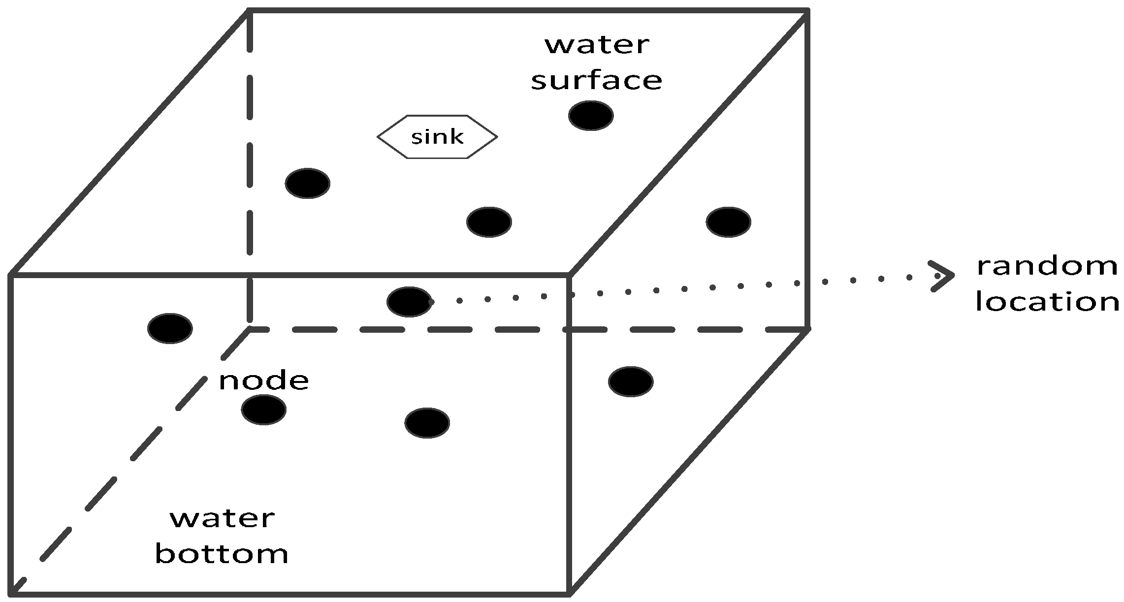
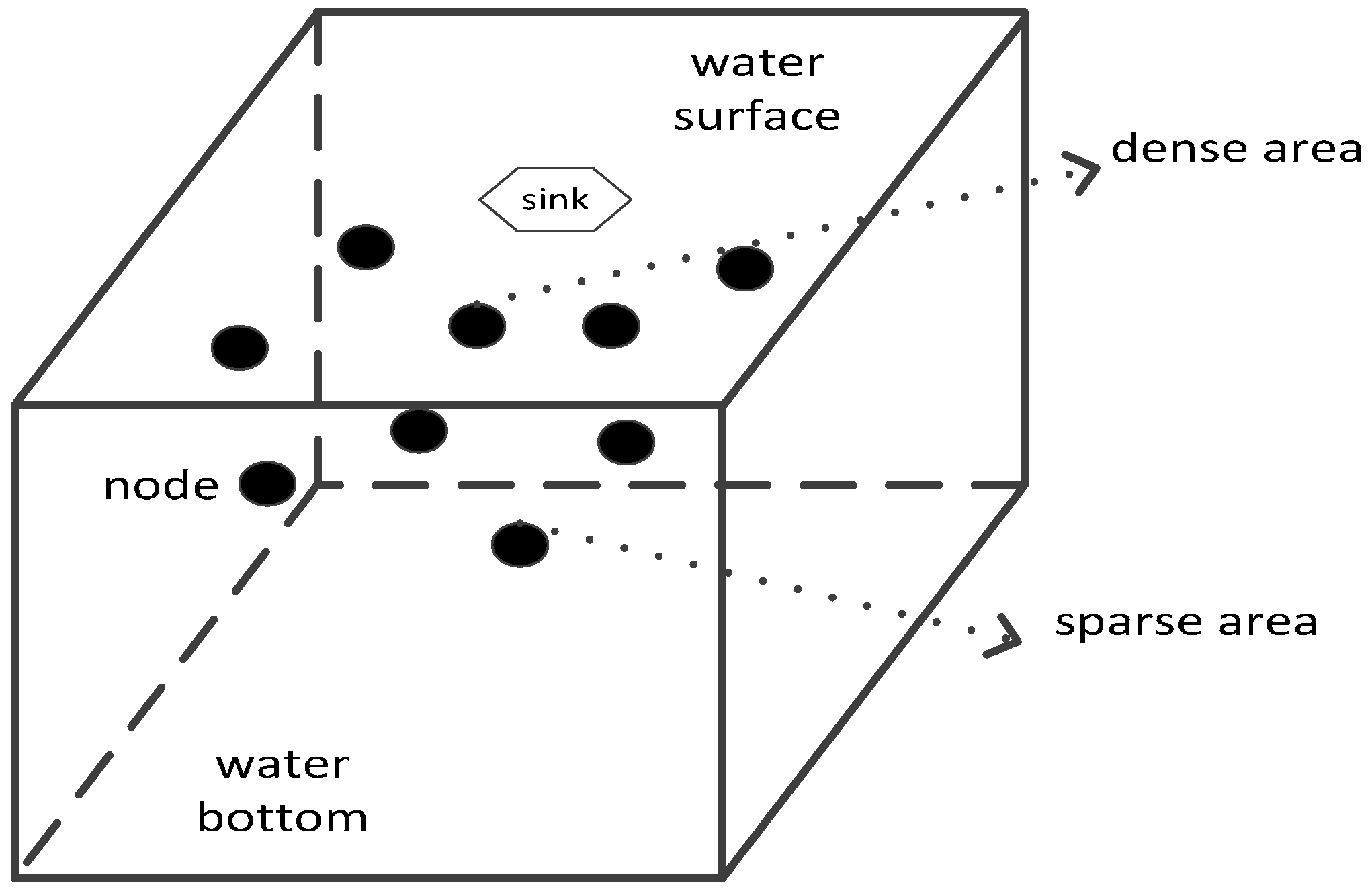
3.2.1. Description of Initial Network Distribution

In this paper, two different initial network distributions are discussed. One initial network distribution is dented as D1 and the other is denoted as D2. The corresponding descriptions about them are given in the following respectively.

Description about initial network distribution D1: As shown in Figure 2, the sink node is fixed at the center of the water surface. All the other sensing nodes are randomly scattered on the surface of the monitored 3D underwater space firstly, then randomly adjust their own depths. Therefore, this initial network distribution is exactly the random distribution and all the sensing nodes have random locations.

Description about initial network distribution D2: As shown in Figure 3, the sink node is fixed at the center of the water surface. As to other sensing nodes, taking node s_j(x_j,y_j,z_j) for example and supposing that the coordinate of the sink node (i.e., the center of the water surface) is (x_sink,_ysink,0), the coordinate of node s_j in the x direction follows the normal distribution whose mean is x_sink and standard deviation is half of the x direction length of the monitored 3D underwater space. Similarly, the coordinate of node s_j in the y direction follows the normal distribution whose mean is y_sink and standard deviation is half of the y direction length of the monitored 3D underwater space. The depth of node s_j (i.e., z_j) can be calculated as follows:

$$\{\begin{array}{l}{d}_{std1}=\sqrt{{\left(x_j-x_{sink}\right)}^2+{\left(y_j-y_{sink}\right)}^2}\\ d_{std2}=\sqrt{{x_{sink}}^2+{y_{sink}}^2}\\ {\mathrm{z}}_j=\frac{d_{std1}}{d_{std2}}*z_h\end{array}$$

(14)

where z_h means the depth of the monitored 3D underwater space. If the network follows the above distribution, the node distribution in the shallow area of the monitored 3D underwater space is denser than that in the deep area. Since the nodes closer to the sink node are usually burdened with heavier information packet forwarding task, this kind of distribution owns the effectiveness in balancing the network energy consumption.

3.2.2. Algorithm Steps

Step 1: The network operation time t is initialized to be 0 round. The network adjustment cycle T_r and node drift cycle T_m are initialized to be two different non-zero constants, and the value of T_r should be larger than that of T_m.

Step 2: t = t + 1 round. Each node senses its own environment and transmits the sensing information to the sink node through single-hop or multi-hop communication. The relay node can compress the received sensing information from other nodes and its own sensing information into one information packet. Judge whether the value of Rem(t,T_r) which means the remainder of dividing t by T_r is 0 or not. If it is, the network operation time reaches the adjustment moment, and the algorithm turns to Step 3 for network topology adjustment; otherwise, the algorithm turns to Step 6.

Step 3: All nodes examine whether they are in the monitored space or not. If all of them are in the monitored space, the algorithm turns to Step 4 (when t = 0, all the nodes are in the monitored space); otherwise, the node outside the monitored space should return to the location recorded in its memory at the last network adjustment moment along the straight line.

Step 4: The sink node set its state at the ready state and all the other nodes set their states at the non-ready states. If node s_i has not received any ready information M_r, it moves to the sink node along the straight line. During the movement, it opens its data receiving module to catch the ready information M_r and stops moving upon the reception of M_r. At the same time, the network is stratified level by level from the sink node. The corresponding description is shown in Figure 4. The process and result are shown in Figure 5 (a network comprised of 9 nodes is taken as the example). After finishing the network stratification, the whole network topology is changed into a stratified connected tree that takes the sink node as the root node, which helps to achieve full network connectivity. In the stratified connected tree, if node s_i has received any acknowledging information M_a, it has one or more child nodes and is considered as a backbone node; otherwise, node s_i has no child node and is considered as a leaf node.

Step 5: After Step 4, the network achieves full network connectivity and the sink node can perform centralized adjustment. First, the sink node determines the set C₁ comprising cube points in the 3D underwater space model, which are less than R_t away (this is helpful to guarantee full network connectivity after centralized optimization) from the backbone nodes in the network. Next, it determines the set C_y comprising the strong leaf nodes in the network. Then, new locations of leaf nodes in C_y are calculated one by one according to the descending order of their residual energy. Taking leaf node s_i for example, p_i and o_i are used to denote its probably new location and old location respectively. First, the sink node calculates its furthest movement distance d_m(i) according to Equation (15):

$$\{\begin{array}{c}{d}_1=\frac{E_i-E_y}{e_{mu}}\\ d_2=\frac{E_i\times r_g}{e_{mu}}\\ d_m(i)=min\left\{d_1,d_2\right\}\end{array}$$

(15)

where d₁ ensures that s_i is still a strong leaf node after reaching the probably new location and d₂ ensures that s_i will not consume excessive energy during the movement (r_g is the control coefficient). Both of them limit the movement energy consumption of the leaf node from different perspectives (d₁ is from the left energy perspective and d₂ is from the consumed energy perspective), therefore, the node movement distance is reduced. Second, the sink node determines set C₂ comprising cube points in the sphere Q_i, whose center is the old location (i.e., o_i) of node s_i and radius is d_m(i). The set C_d = C₁∩C₂ is calculated. Next, the sink node considers cube points in C_d one by one. Taking cube point p_i for example, the network coverage rate is C_v(o_i) when node s_i is at its old location o_i, and would be C_v(p_i) if node s_i moved to its probably new location p_i. The distance between o_i and p_i is denoted as d(o_i,p_i). The target cube point p_d(s_i) (i.e., final destination location of node s_i) is calculated according to Equation (16). The sink node returns the result information to node s_i, and node s_i moves to p_d(s_i) along the straight line. Then, the sink node considers the next strong leaf node until all the strong leaf nodes have been studied. After this, all the nodes record the real-time locations into their own memories.

$$\{\begin{array}{c}{p}_d(s_i)=\underset{p_i\in C_d}{\max }\left\{\frac{\Delta C_v(o_i,p_i)}{d(o_i,p_i)}\right\}\\ \Delta C_v(o_i,p_i)=C_v(p_i)-C_v\left(o_i\right)>0\end{array}$$

(16)

Step 6: The fact that whether Rem(t,T_m) (remainder of dividing t by T_m) is 0 or not determines whether the node drift with water environment occurs in the current network operation time. If the value of Rem(t,T_m) is 0, all the nodes drift according to the 3D random drift model; otherwise, the algorithm turns to Step 7.

Step 7: The sink node calculates the network coverage rate and judges whether the network reaches the network lifetime or not. If it is, the algorithm ends; otherwise, the algorithm turns to Step 2.

3.2.3. Detailed Description for Algorithm Important Parts

To give a better understanding about the proposed algorithm, the following important parts of the NRBSCT algorithm will be elaborated in detail and with examples. Supposing that the scenery is the same with that described in the following simulation setup, and the network adjustment cycle T_r and node drift cycle T_m are initialized to be 50 rounds and 5 rounds respectively. The network operation time just comes to 50 rounds, i.e., the first adjustment moment. At this time, the algorithm will turn to Step 3 which is mentioned in the previous part for network topology adjustment. We will take the scenery at this time as an example to describe for simplicity.

Self-Examination and Adjustment of Nodes Outside the Monitored Space

Since the network operation time is just 50 rounds, actually all the nodes have drifted according to the 3D random drift model 9 times, which occurred at Rounds 5, 10, 15, 20, 25, 30, 35, 40, and 45. It is possible that some nodes may drift outside the monitored space. Taking node s_e as the example, as is shown in

Table 2. Location changes of node s_e.

Round	0	40	49	50 (after Adjustment)
Location	(115, 37, 16)	(123, 41, 19)	(125, 43, 21)	(115, 37, 16)
Inside/Outside	Inside	Outside	Outside	Inside

, it gradually drifted outside the monitored space, so it returns to the location recorded in its memory at the last network adjustment moment. Since the network operation time is just the first adjustment moment, the last network adjustment moment means the operation starting time (i.e., when t = 0). Therefore, node s_i will move from (125, 43, 21) to (115, 37, 16), which makes itself come back into the monitored space to help maintain good network monitoring quality.

Network Connectivity Rate Improvement

After Step 3, all the nodes have been into the monitored space. However, because of the initial random deployment and previous drift caused by the water environment, some nodes fail to communicate with the sink node through single-hop or multi-hop communication, which means that the network cannot still achieve full network connectivity. Therefore, measures should be taken to improve the network connectivity, and it is better to achieve full network connectivity if possible. Taking the scenery shown in Figure 5 as an example, 9 nodes in the network finally form a stratified connected tree whose root node is the sink node with the method described in Figure 4 in Step 4. This is one aspect of improve the network connectivity rate for the NRBSCT algorithm. As to the other aspect, in the centralized adjustment performed by the sink node in Step 5, the target cube point p_d(s_i) (i.e., final destination location of strong leaf node s_i) belong to the set C_d = C₁∩C₂, which means it also belongs to the set C₁ and is less than R_t away from the backbone nodes in the network, which is helpful to guarantee full network connectivity after centralized optimization. The scenery shown in Figure 5 can also be the example. Figure 5 shows that after the network stratification, nodes s₂, s₃, s₈ and s₉ are the leaf nodes. Supposing that their left energy are distributed as

Table 3. Left energy description.

Node	s2	s3	s8	s9
Left energy (J)	75	61	77	57
Inside/Outside	Inside	Outside	Outside	Inside
Strong leaf node	Yes	No	Yes	No

shows (the simulation value at the 50 round time is much bigger than the supposition value in Table 3), since the energy threshold E_y = E_tx(R_t) × T_r is 65 J in the currently supposed simulation scenery, nodes s₂ and s₈ can be treated as the strong leaf nodes. Therefore, based on Equations (15) and (16), the sink node firstly determine the final destination location for node s₂, and then for node s₈.

Node Movement Distance Limit

During the calculation of the final destination location for the strong leaf node, it is necessary to consider how to limit the node movement distance, since the movement energy consumption is huge and node energy is limited and difficult-to-supplement in the water environment. Therefore, in Equations (15) and (16), measures are taken to limit the node movement distance. Taking node s₈ as the example, in Equation (15), the calculation of d₁ (value is 8 m) limits the movement distance by ensuring that node s₈ is still strong after the current movement; while the calculation of d₂ (value is 10 m) limits the movement distance by ensuring that node s₈ will not consume excessive energy during the current movement. By using Equation (16), the node movement distance is also limited when requiring the node to move toward its final destination location to improve the network coverage rate. As is shown in Figure 6, point p₁ and p₂ belong to the set C_d = C₁∩C₂. If node s₈ chooses p₁ as its final destination location, it should move 6 m to gain 0.035 network coverage rate improvement; however, if node s₈ chooses p₂ as its final destination location, it should move 4 m to gain 0.025 network coverage rate improvement. Since moving toward p₂ can gain more network coverage rate improvement per movement distance, node s₈ will prefer to choose p₂ rather than p₁.

Overall Summarization for Main Mathematical Symbols

Since there are a large number of mathematical symbols, to give a better description of these symbols,

Table 4. Main mathematical symbols.

Symbols	Meanings
w	cube side length
d	transmitting distance of information package
Mb	size of information package
Tp	transmitting time of information package
Sv	transmission speed of information package
f	carrier acoustic signal frequency
α(f)	water absorption coefficient
A(d)	energy attenuation
λ	energy spreading factor
Etx(d)	energy consumption for transmitting information
Pr	power threshold for receiving information package
tn	information package transmitting times for a node
Rt	communication range
Ce	communication energy consumption
Me	movement energy consumption
md	movement distance
mu	energy consumption per movement distance
Pe	controlling probability of node drift
Cv	network coverage rate
Pc	number of cube points covered
Pt	total number of all cube points
Cn	network connectivity rate
nc	number of nodes being able to communicate with sink node
n	number of all nodes
t	network operation time
Tr	network adjustment cycle
Tad	network adjust moment
Ei	energy of node si
Ed	energy threshold judging death of node
Ey	energy threshold judging whether leaf node is strong enough
Lf	network lifetime
Cth	coverage rate threshold
Ein	node initial energy
Rs	sensing range
Tm	node drift cycle
Mr	ready information
Ma	acknowledging information
rg	control coefficient

includes main mathematical symbols used.

3.2.4. Algorithm Analysis

For the 3D underwater space model, whether a small cube is covered or not depends on the covering state of its center point. Therefore, for the NRBSCT algorithm, when the sink node performs centralized optimization to adjust the locations of leaf nodes, the cube resolution w affects the calculating accuracy and time complexity of centralized optimization. If w is small, the calculating accuracy and time complexity is high. For example, when the sink node calculates the final destination location for node s_i, it has to calculate C_v(o_i) and C_v(p_i), and the time complexities for these two calculations are the same, i.e., O(P_t × n). The smaller w means the larger P_t, and then results in the higher time complexity.

4. Simulation Evaluation

4.1. Algorithm Comparison and Evaluation Metrics

Though the MRNR algorithm seems to be a little old, it seems the only one that can be found to solve the node redeployment problem researched in this paper as far as we know after our deep and extensive literature study; thus, to evaluate the proposed NRBSCT algorithm reasonably, the MRNR algorithm is chosen for comparison. The performances of MRNR and NRBSCT algorithms are compared from the following metrics: the number of nodes in the monitored 3D underwater space, network coverage rate, network connectivity rate, and network lifetime.

Compared with the MRNR algorithm, the NRBSCT algorithm has some advantages, as follows:

(1)

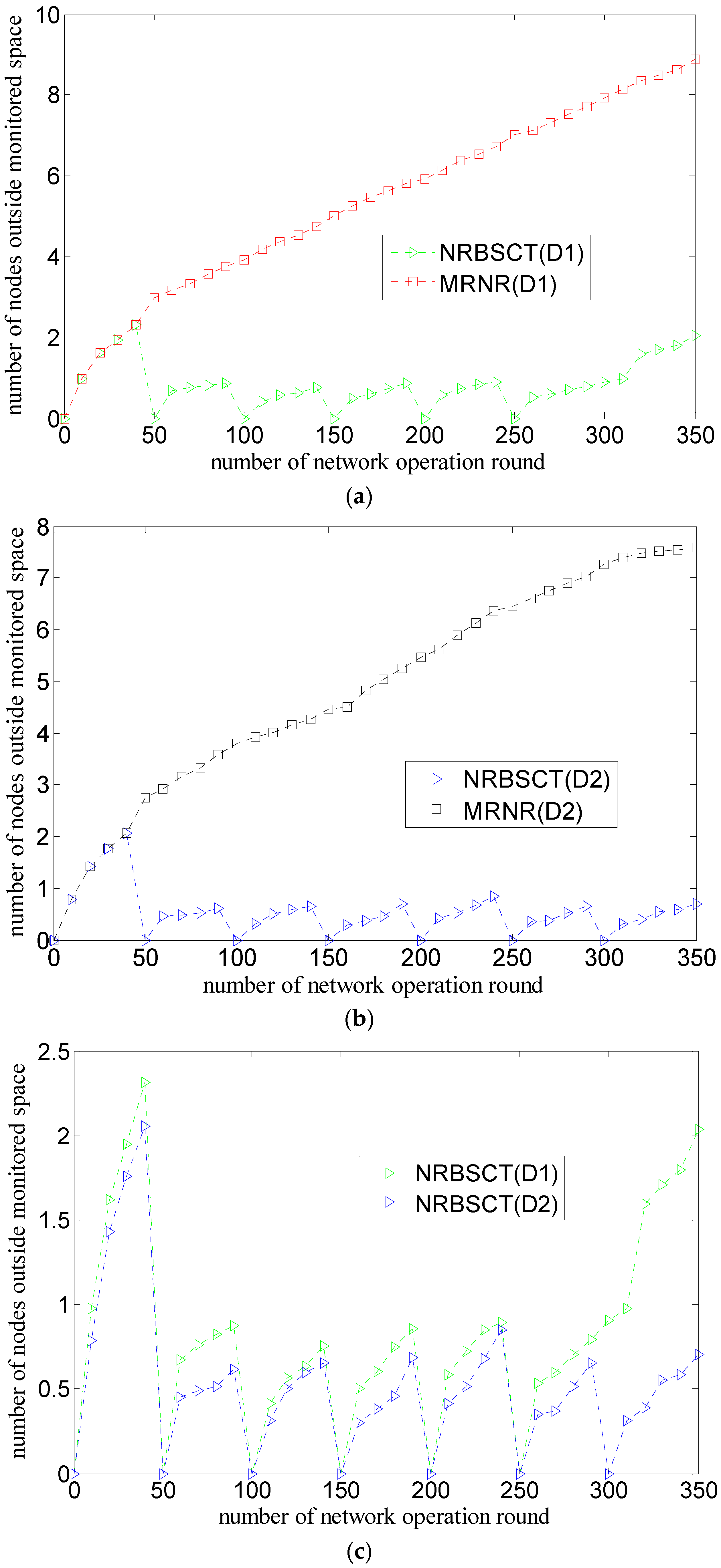
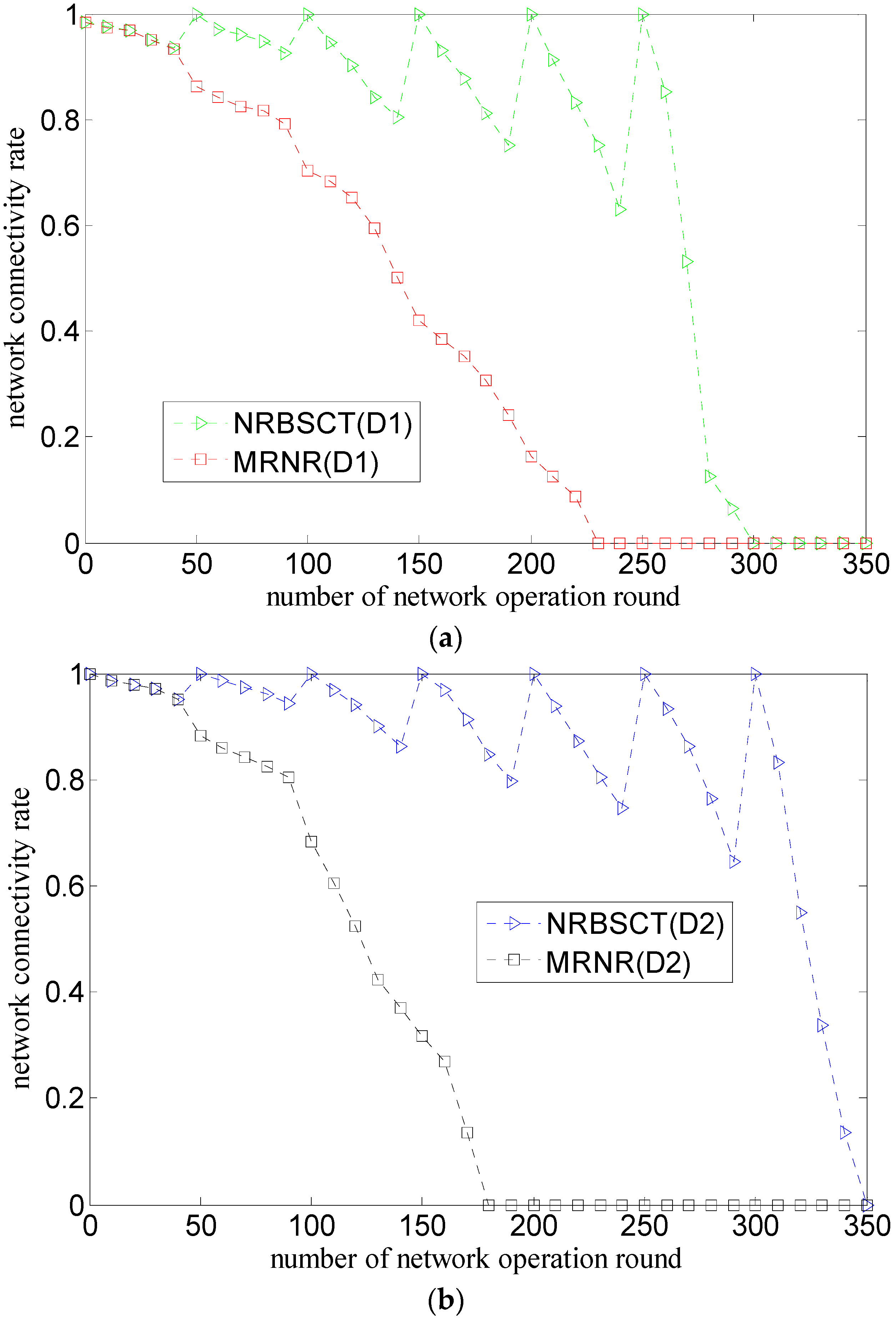
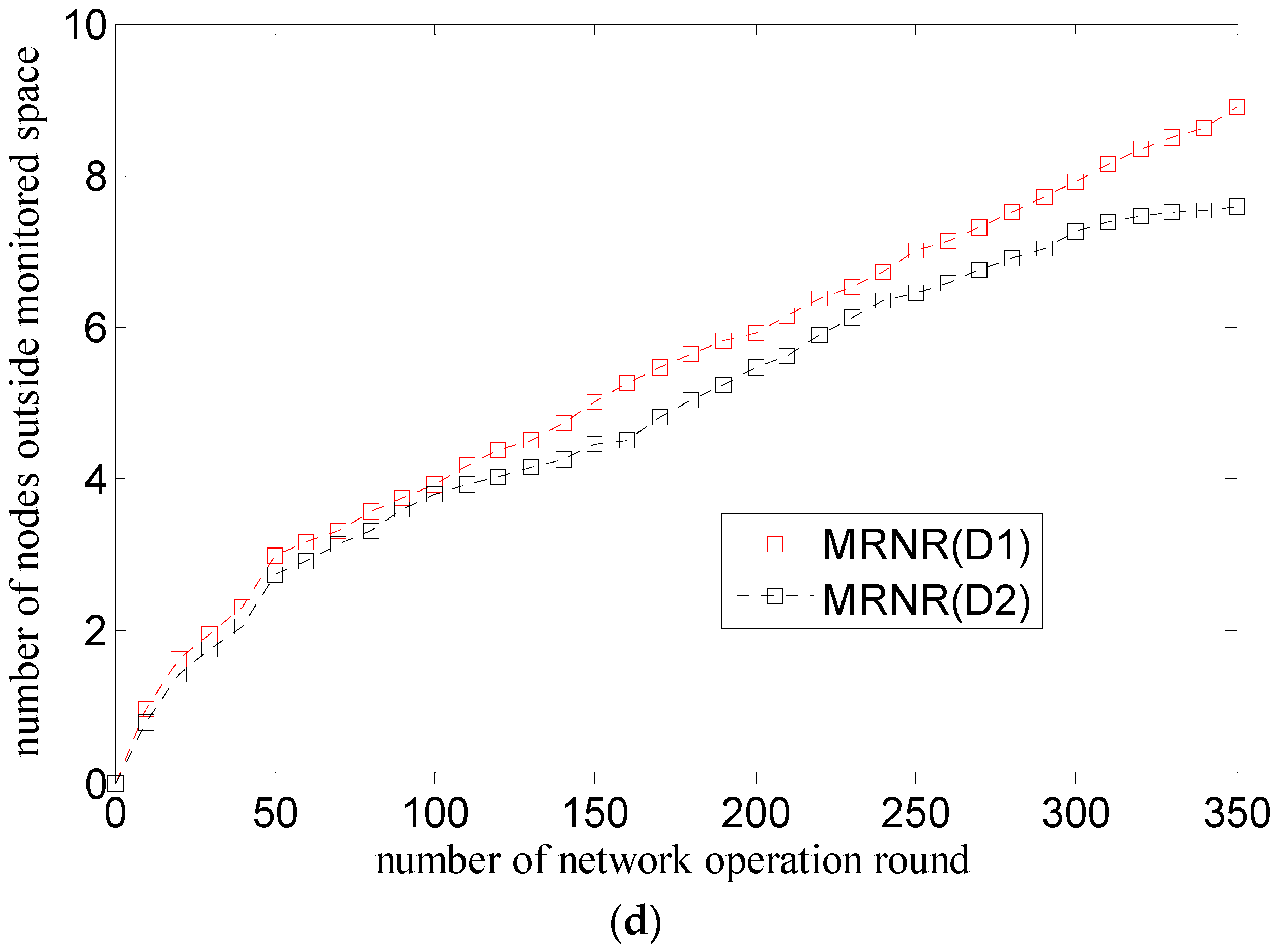
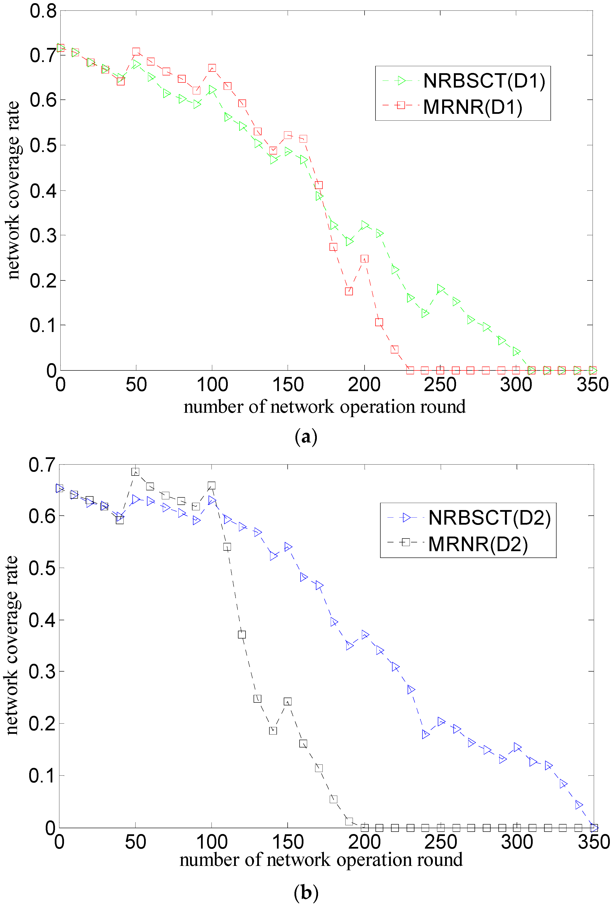
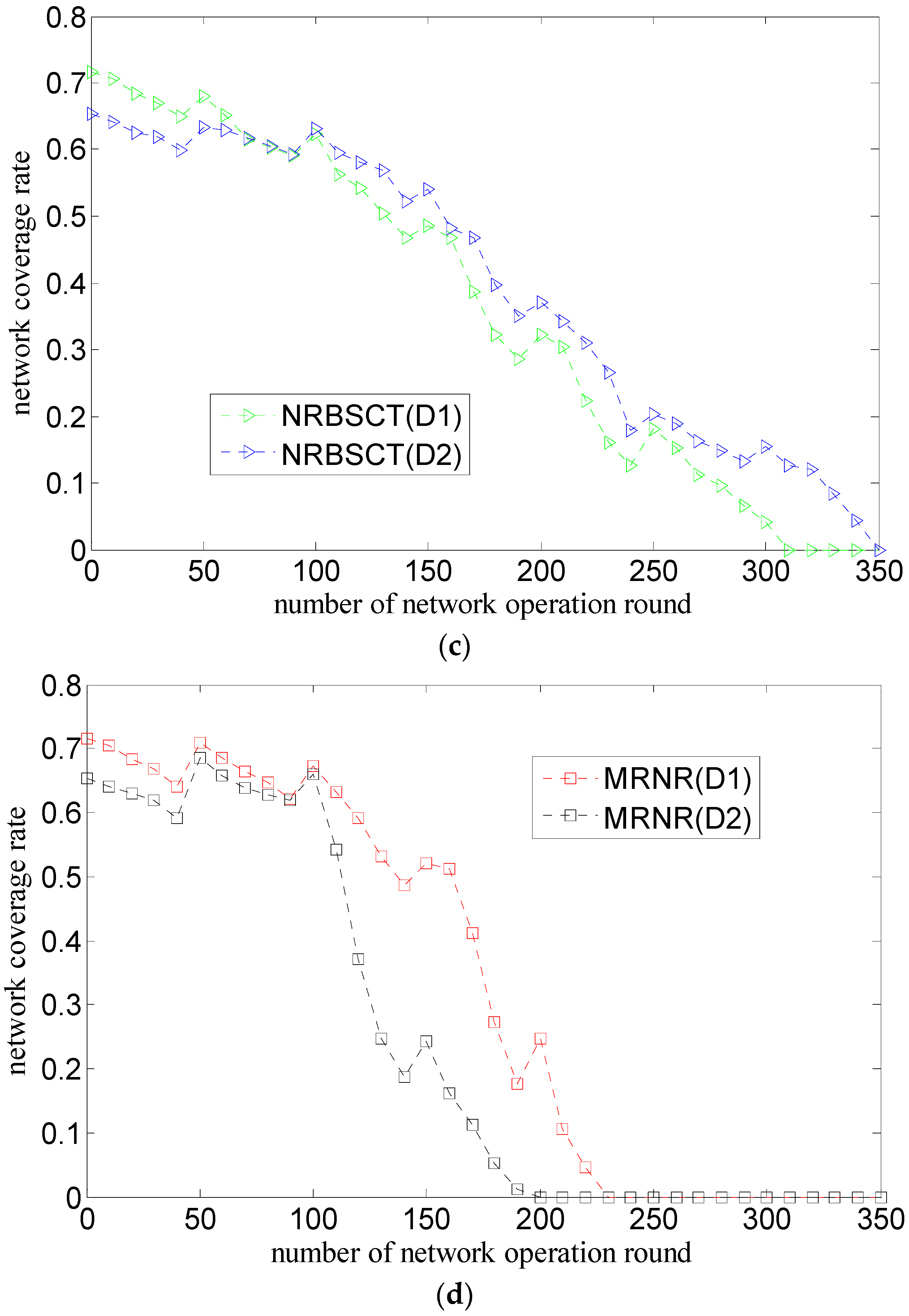
The MRNR algorithm does not propose effective measures to prevent nodes from drifting out of the monitored space because of water environment. However, the NRBSCT algorithm can make nodes outside the monitored space return back through self-examination and adjustment on node locations, which is goodfor maintaining good network monitoring quality.

(2)

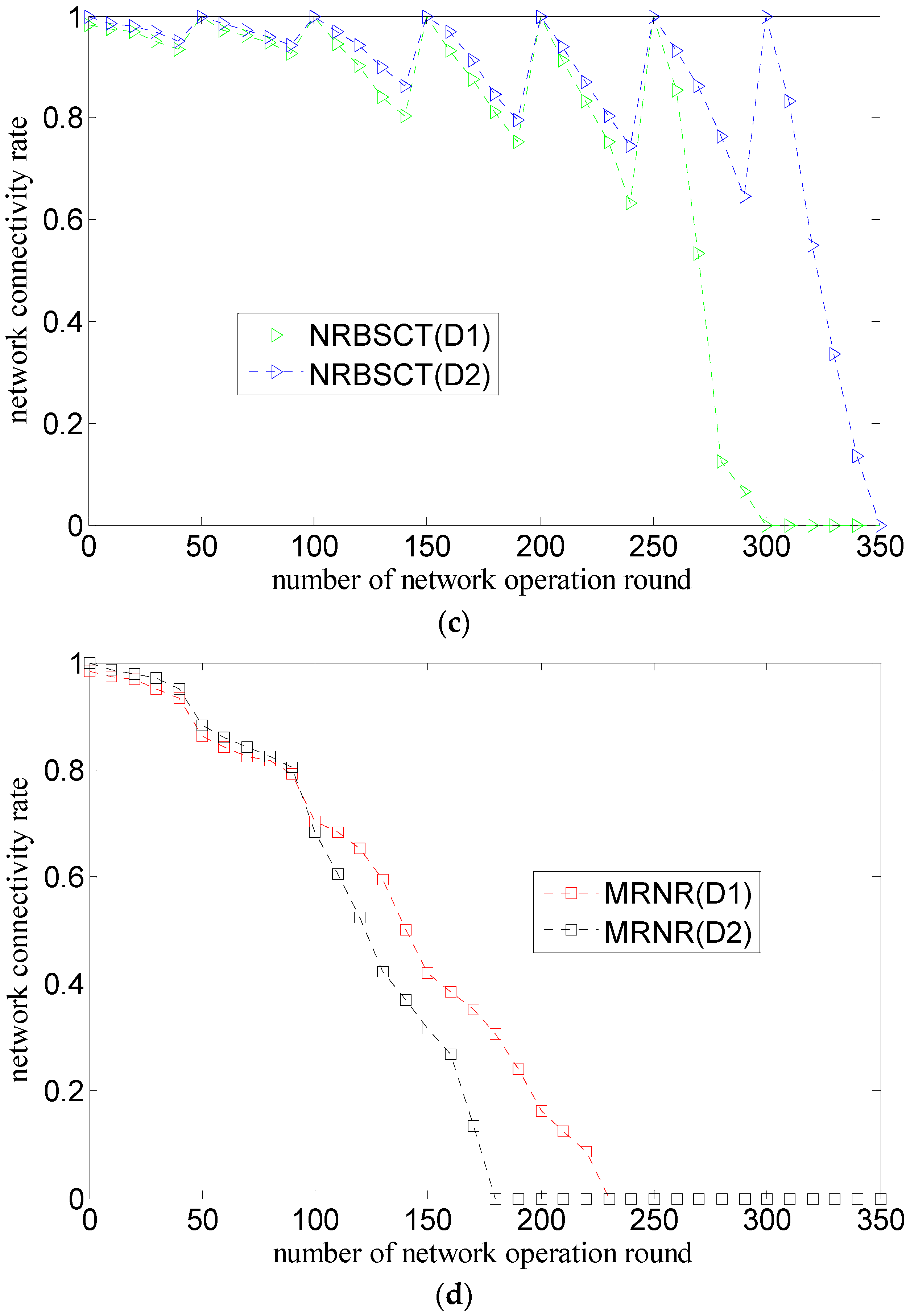
The MRNR algorithm only considers how to improve the network coverage rate, but ignores the network connectivity rate improvement. However, at the network adjustment moment, the NRBSCT algorithm can firstly establish a stratified connected tree that takes the sink node as the root node, and then ensure that in the centralized optimization conducted by the sink node, the final destination location of node s_i will not be R_t away from the backbone nodes, which achieves full network connectivity and also helps to maintain a relatively high network connectivity during network operation.

(3)

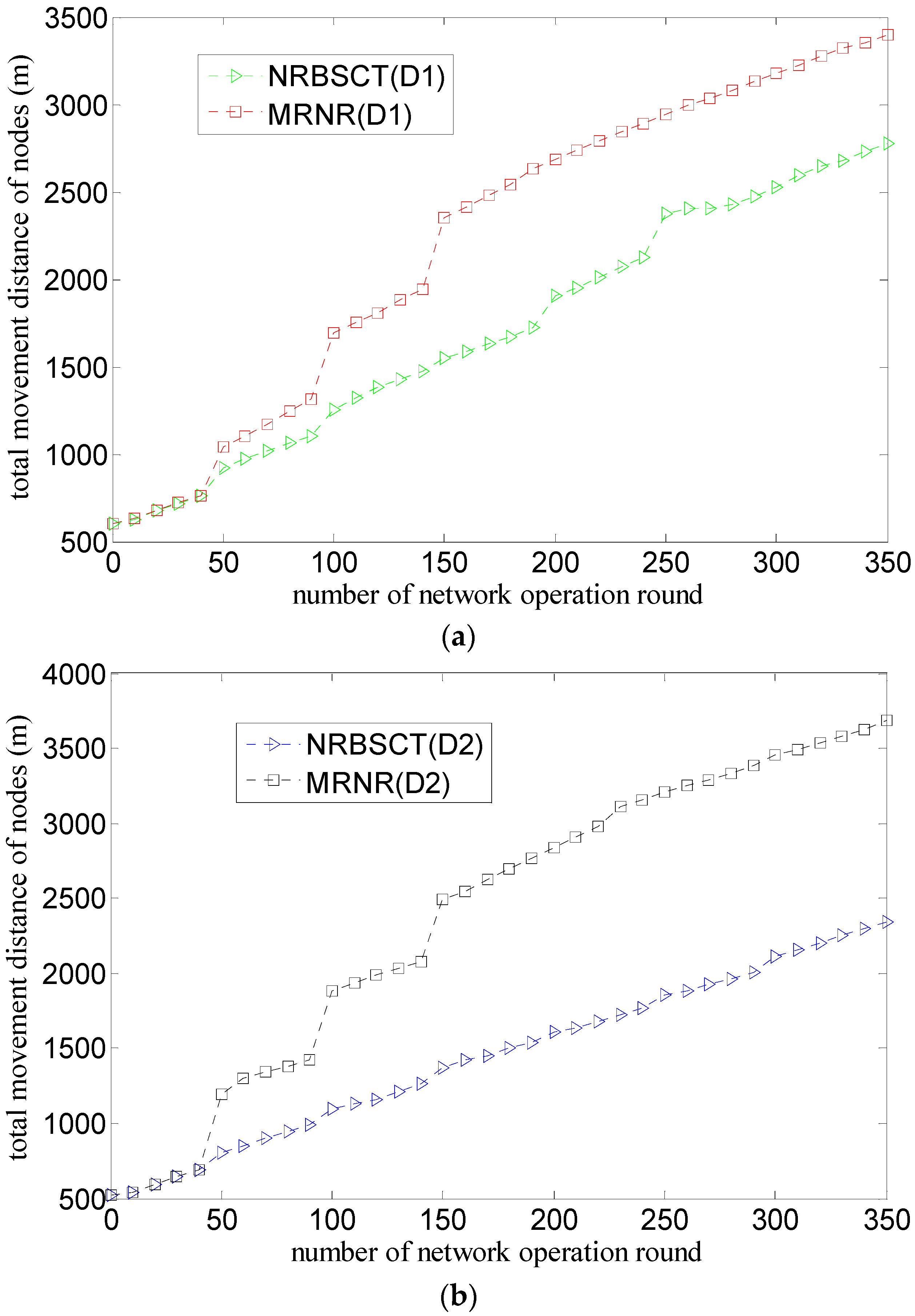
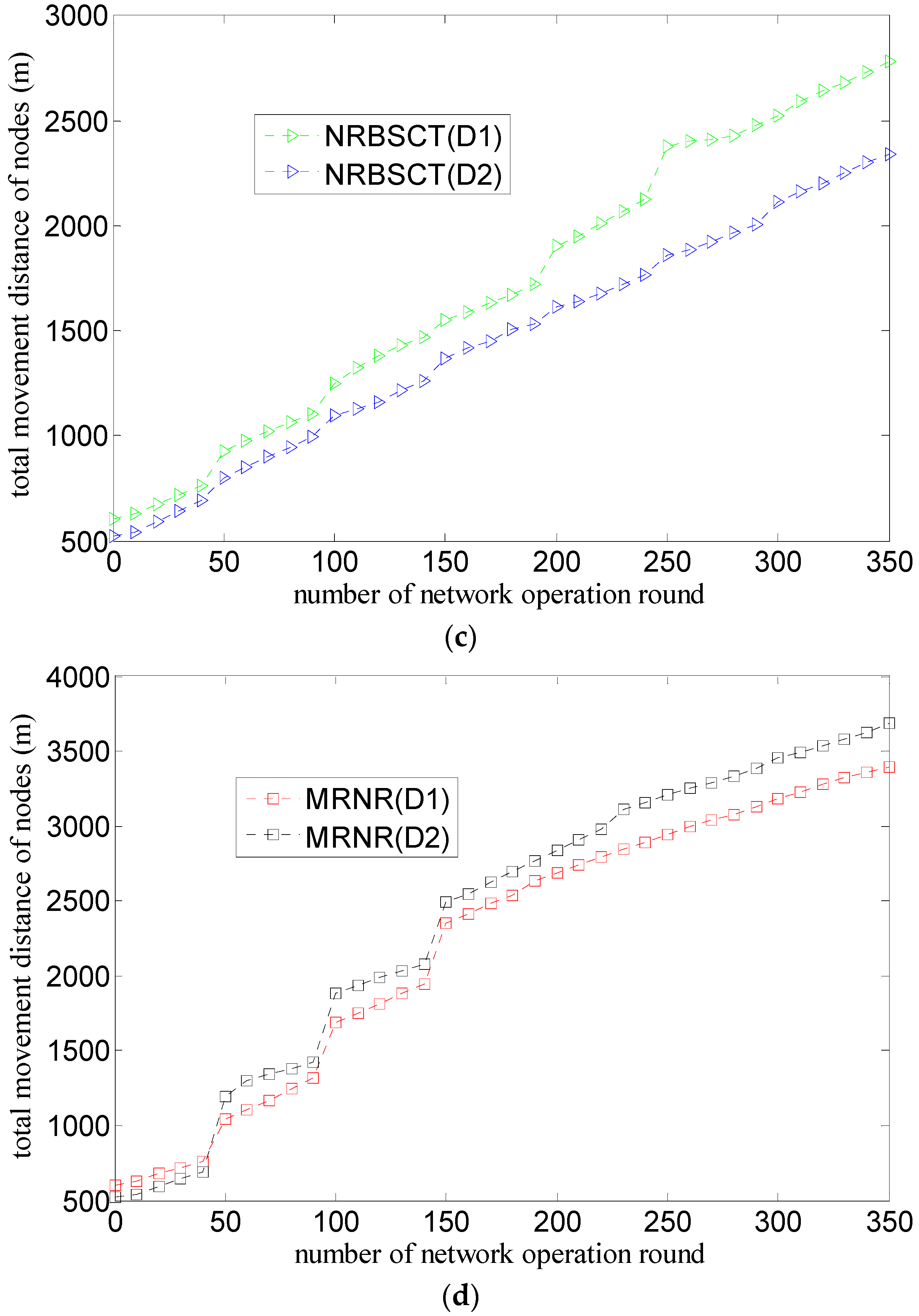
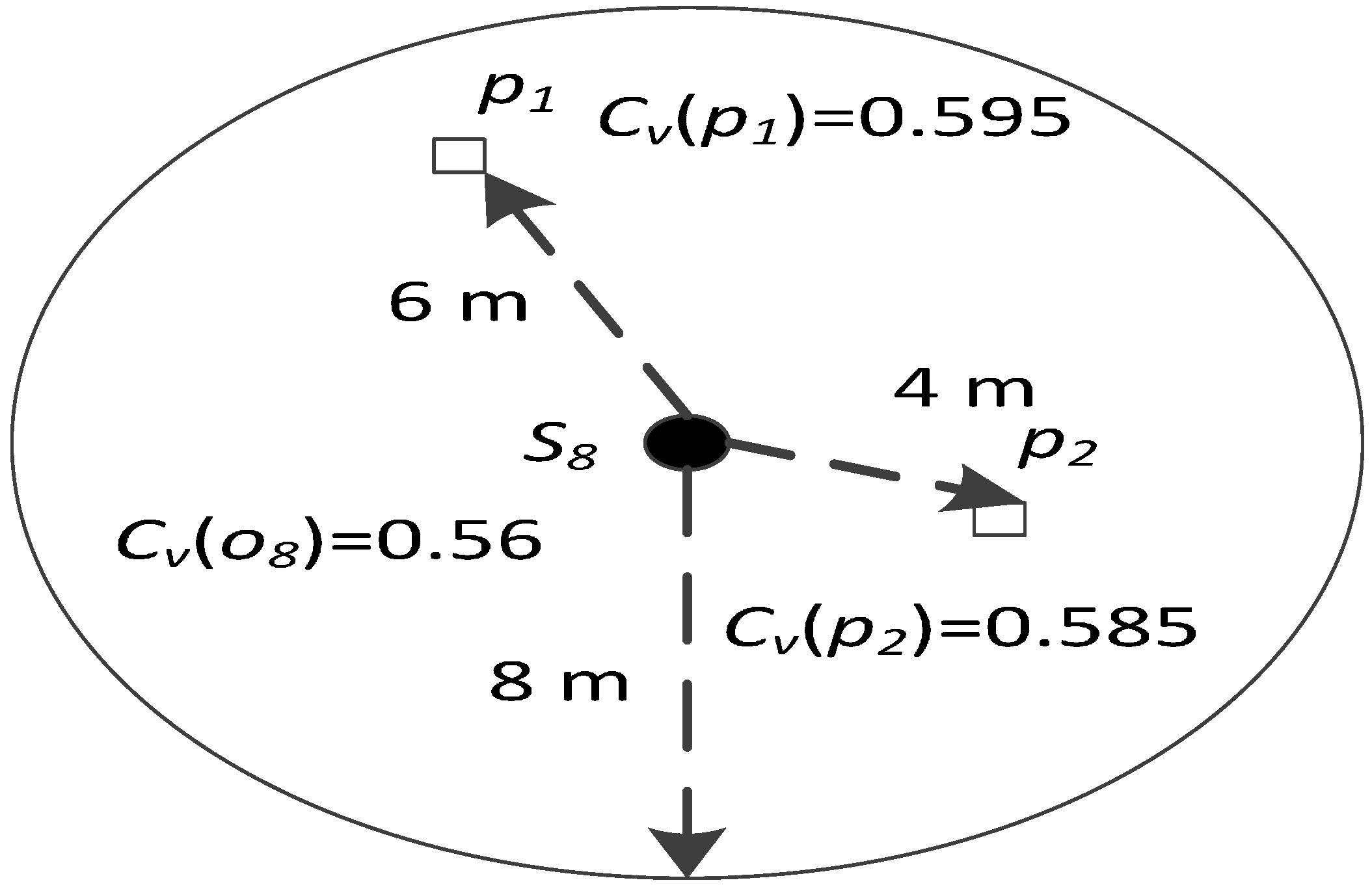
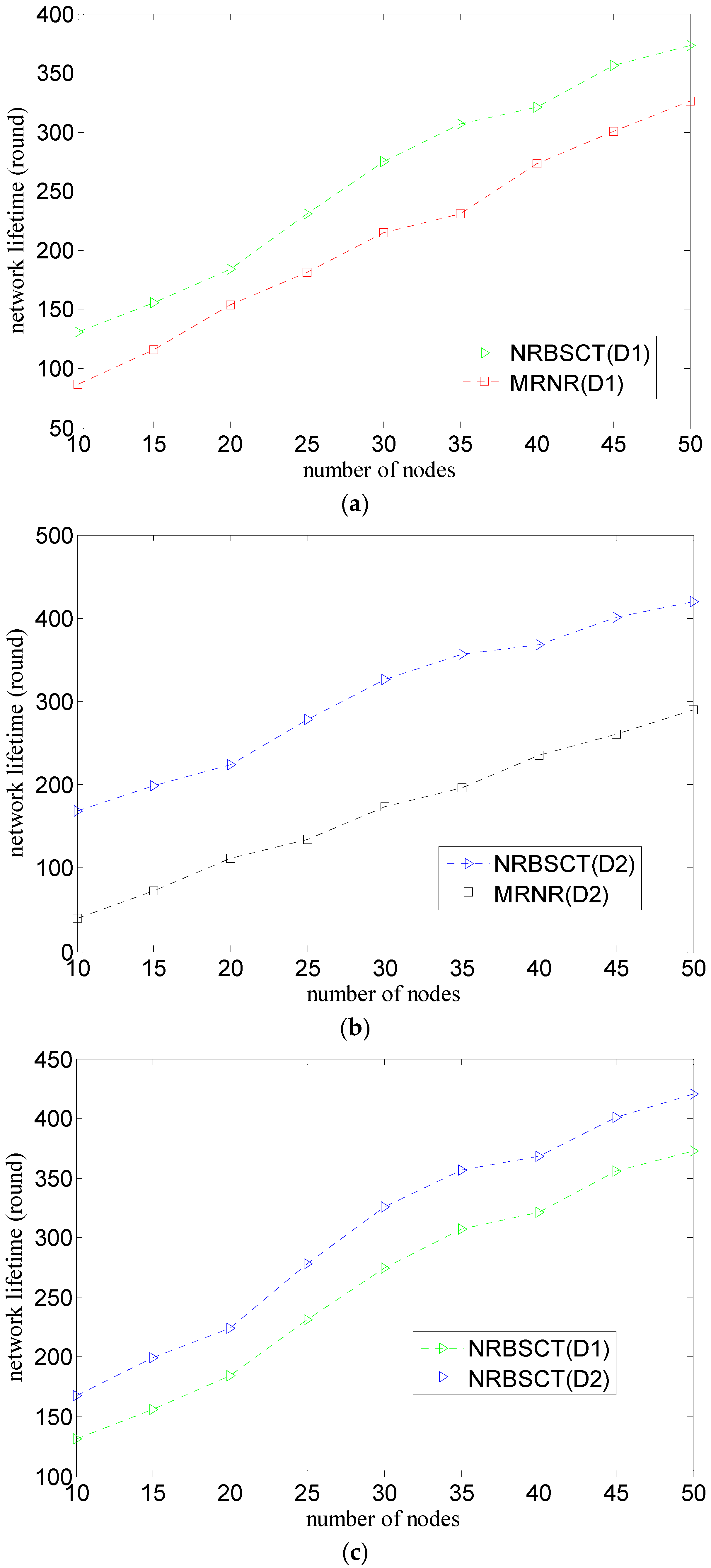
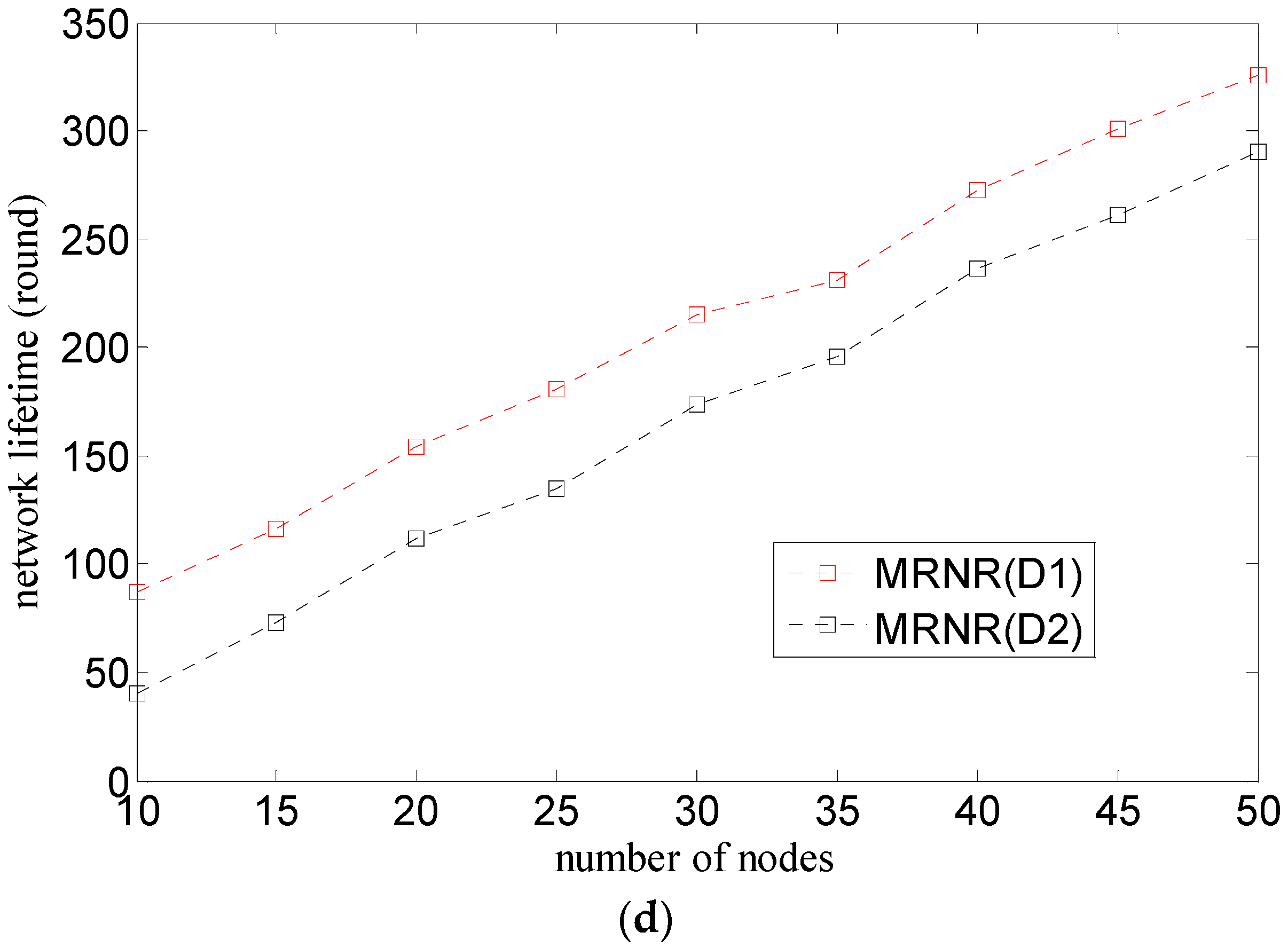
The MRNR algorithm does not consider how to shorten the movement distance when requiring the least important node to move toward the biggest coverage blind point to improve the network coverage rate. However, the centralized optimization conducted by the sink node in the NRBSCT algorithm considers limiting node movement distance from the left and consumed energy perspectives, which can shorten the total movement distance of nodes during redeployment and prolong the network lifetime.

4.2. Simulation Scenario and Parameter Settings

Matlab software is used to simulate the algorithms. The final results shown in the following figures are the averages of 50 times to eliminate the effect of simulation randomness. The length and width in the horizontal direction of simulative monitored 3D underwater space are the same, i.e., 120 m, whereas the depth of space is 60 m. The cube resolution w is 5 m. In the 3D random drift model, node maximum drift distances along the x, y and z directions are controlled by setting m_x = m_y = m_z = 1 and λ₁ = 0.8. Node drift probability P_e is set to be 0.3, and drift probabilities along the positive directions of x, y and z axes are controlled by setting P_dx = P_dy = P_dz = 0.5. In the NRBSCT algorithm, the value of r_g is 0.2. Other main parameter settings of the MRNR and NRBSCT algorithms are enumerated in

Table 5. Parameter settings.

Parameter Names	Parameter Values
Initial energy of node (Ei)	500 J
Network coverage rate threshold (Cth)	0.1
Energy consumption per movement distance (mu)	1.5 J/m
Size of information package (Mb)	1 Kbit
Receiving Power threshold (Pr)	0.05 w
Frequency of carrier acoustic signal (f)	25 kHz
Transmission speed of information package (Sv)	5 kbps
Energy spreading factor (λ)	1.5
Sensing range of node (Rs)	15 m
Communication range of node (Rt)	25 m
Network adjustment cycle (Tr)	50 round
Node drift cycle (Tm)	5 round

.

4.3. Simulation Results and Analysis

Figure 7 shows the comparison of the relationship between the number of nodes outside the monitored space and the round of network operation considering both the initial network distribution (D1 or D2) and the network redeployment algorithm (MRNR or NRBSCT), where the number of nodes is 30.

As shown in Figure 7a,b, node may drift with water environment during network operation. For the MRNR algorithm, more and more nodes drift outside the monitored space during network operation; however, for the NRBSCT algorithm, the number of nodes outside the monitored space does not increase too much, moreover, the NRBSCT algorithm can almost keep all the nodes in the monitored space when the network operation time (not exceeding the network lifetime) is just the network adjustment moment. The reason is that the MRNR algorithm does not propose any methods to prevent nodes from drifting outside the monitored space because of water environment; however, the NRBSCT algorithm can drive nodes outside the monitored space to move back into the monitored space through self-examination and adjustment on node locations, which is significant to help the network maintain better monitoring quality.

As shown in Figure 7c,d, for both the MRNR algorithm and the NRBSCT algorithm, compared with the initial network distribution D1, since there are more nodes distributed in the area around the sink node and less nodes distributed in the area near the boundary of the monitored water space for the initial network distribution D2, less nodes will move out of the monitored water space during the network operation.

Figure 8 shows the comparison of the relationship between the network coverage rate and the round of network operation considering both the initial network distribution (D1 or D2) and the network redeployment algorithm (MRNR or NRBSCT), where the number of nodes is 30.

As shown in Figure 8a,b, for both of these algorithms, the network coverage rates will decrease during network operation from the whole. The reason is that some nodes drift out of the monitored space and some nodes die from energy depletion. However, when the network operation time is just the network adjustment moment, both of these two algorithms can contribute to the network coverage rate improvement to some extent since they propose the corresponding methods. Specifically, at the beginning of network operation (i.e., from the start to the 176 rounds for the initial network distribution D1 and to the 103 rounds for the initial network distribution D2), the MRNR algorithm can always achieve a higher network coverage rate than the NRBSCT algorithm; however, at the end of the network operation, the network coverage rate for the MRNR algorithm degrades dramatically with a relatively short network lifetime (i.e., 215 rounds for the initial network distribution D1 and 174 rounds for the initial network distribution D2), and that for the NRBSCT algorithm can remain a certain level for a longer network lifetime (i.e., 275 rounds for the initial network distribution D1 and 326 for the initial network distribution D2). The reason is that the MRNR algorithm only focuses on maximizing the network coverage rate, which results in a higher network coverage rate; however, compared with the MRNR algorithm, the proposed NRBSCT algorithm not only considers how to keep nodes from drifting out of the monitored space, but also tries to shorten node movement distance when the sink node conducts centralized optimization on leaf node locations, which can help to save movement energy consumption and keep the network coverage rate at a certain level for a longer network lifetime.

As shown in Figure 8c,d, for the NRBSCT algorithm, compared with the initial network distribution D1, since the nodes in the initial network distribution D2 tends to be located in the area near the sink node, which results more coverage overlaps, the network coverage at the beginning of network operation (i.e., from the start to the 78 rounds) is relatively lower. However, the initial network distribution D2 also results in less moving-out nodes during network operation and less movement distance during the network redeployment, which helps a lot to save the node movement energy consumption, so more nodes will save their energy to contribute to higher network coverage rates and the network lifetime can be prolonged from 275 rounds in the case of initial network distribution D1 to 326 rounds in the case of initial network distribution D2. However, that regularity cannot hold for the MRNR algorithm, since compared with the initial network distribution D1, the initial network distribution D2 is exactly less uniform, which not only means that there exists more coverage overlaps in the initial network operation, but also causes that more nodes will be involved in the network redeployment process, moving from the dense area close to the sink node to the sparse area far away from the sink node. Because of the relatively large movement energy consumption, too much movement distance will result in large movement energy consumption, which makes nodes die faster and degrades the network coverage rate. For the above reasons, the network coverage for the MRNR algorithm in the case of initial network distribution D2 cannot exceed that in the case of initial network distribution D1.

Figure 9 shows the comparison of the relationship between the network connectivity rate and the round of network operation considering both the initial network distribution (D1 or D2) and the network redeployment algorithm (MRNR or NRBSCT), where the number of nodes is 30.

As shown in Figure 9a,b, for the MRNR algorithm, the network connectivity rate will decrease during network operation from the beginning to the network lifetime. The reason is that on the one hand, some nodes drift out of the monitored space and some nodes die from energy depletion; on the other hand, the MRNR algorithm only focuses on maximizing the network coverage rate and ignores how to slow the network connectivity rate decrease. However, for the NRBSCT algorithm, the network connectivity exhibits some fluctuations during its decrease. The reason for this is actually the consideration of slowing the network connectivity rate decrease. Specifically speaking, if the network operation time is not the network adjustment moment T_ad, the network connectivity exhibits the decrease because of the node drift caused by water environment and node death caused by energy depletion. While, if the network operation time is just the network adjustment moment T_ad (such as 50 rounds, 100 rounds, 150 rounds), the NRBSCT algorithm can firstly establish a stratified connected tree that takes the sink node as the root node, and then ensure that in the centralized optimization, the final destination location of node s_i will not be R_t away from the backbone nodes, which achieves full network connectivity and makes the value of the network connectivity bigger than that of the former or latter network operation time (i.e., the network connectivity exhibits the fluctuation phenomenon).

As shown in Figure 9c,d, for the NRBSCT algorithm, compared with the initial network distribution D1, the network connectivity rate in the case of the initial network distribution D2 is relatively higher, which may be the result of the fact that the majority of nodes in the initial network distribution D2 tend to be located in the area near the sink node. However, the same regularity can only hold for a short network operation time for the MRNR algorithm (i.e., 98 rounds), the reason is that at the network adjustment moments, in order to increase the network coverage rate, the MRNR algorithm requires nodes in the dense area near the sink node to move to the sparse area far away from the sink node, which will degrade the network connectivity.

Figure 10 shows the comparison of the relationship between the total movement distance of nodes in the network and the round of network operation considering both the initial network distribution (D1 or D2) and the network redeployment algorithm (MRNR or NRBSCT), where the number of nodes is 30.

As shown in Figure 10a,b, the total movement distance of nodes will increase during network operation from the whole for both algorithms. The reason is that, on the one hand, nodes may drift with water environment; on the other hand, both redeployment algorithms require some nodes to move toward better locations to improve network monitoring quality when the network operation time is just the network adjustment moment. Compared with the former, the latter will cause larger movement distance, which can be demonstrated with the higher curve slopes at the network adjustment moments. However, the total movement distance for the NRBSCT algorithm is smaller than that of the MRNR algorithm, the reason is that compared with the latter, the former considers how to decrease the node movement distance from the left and consumed energy perspectives when the sink node conducts centralized optimization on the locations of leaf nodes, which avoids the large-scale node movement that may occur in the latter.

As shown in Figure 10c,d, for the NRBSCT algorithm, compared with the initial network distribution D1, the total movement distance of nodes in the network in the case of the initial network distribution D2 is relatively smaller, and there are two main reasons accounting for this phenomenon. Firstly, the movement of nodes in the formation of the initial network distribution D2 is comparatively smaller than that of the initial network distribution D1, since the majority of all the nodes only need a relatively small depth adjustment. Secondly, in the case of the initial network distribution D2, based on the fact that the majority of all the nodes are located in the area near the sink node and the minority of all the nodes are located in the area far away from the sink node, both the number of node moving out of the monitored space and the node movement distance produced in process of the network redeployment at the network adjustment moments are relatively smaller. However, for the MRNR algorithm, the same regularity can only hold for a short network operation time (i.e., before the 50 rounds) owning to the first reason mentioned above. Once the network operation time comes to the network adjustment moment, large numbers of node in the dense area near the sink node will be required to move towards the sparse area far away from the sink node for the purpose of increasing the network coverage rate, which will obviously cause larger node movement distance increase than that in the case of the initial network distribution D1.

Figure 11 shows the comparison of the relationship between the network lifetime and the number of nodes considering both the initial network distribution (D1 or D2) and the network redeployment algorithm (MRNR or NRBSCT), where the number of nodes varies from 10 to 50.

As shown in Figure 11a,b, compared with the MRNR algorithm, when the network scale is the same (i.e., the number of nodes is the same), the NRBST can always achieve a higher network lifetime. The reason is that when the sink node conducts centralized optimization, the MRNR algorithm only considers maximizing the network coverage rate, with node movement distance ignored; while the NRBSCT algorithm considers how to not only improve the network coverage and connectivity rates, but also decrease node movement distance (this is also shown in Figure 10). Since node movement energy consumption in water environment is much larger than other kinds of energy consumption, the node movement distance decrease will produce a significant network lifetime improvement.

As shown in Figure 11c,d, compared with the initial network distribution D1, when the network scale is the same (i.e., the number of nodes is the same), the network lifetime in the case of the initial network distribution D2 is relatively longer for the NRBST algorithm and is relatively shorter for the MRNR algorithm. This phenomenon also results from the facts that node movement energy consumption accounts for large percent of the total energy consumption of a node. Furthermore, it is easy to understand this phenomenon considering the total node movement distance shown in Figure 10.

5. Conclusions and Future Work

A NRBSCT algorithm is proposed because improving the network coverage and connectivity rates at the cost of the probably minimal node energy consumption to maintain excellent network monitoring quality as long as possible with full consideration of node drift with water environment is difficult for existing UWSNs node redeployment algorithms. At every network adjustment moment, nodes firstly perform the self-examination and adjustment on locations to keep themselves in the monitored space, which ensures that number of nodes in the monitored space can be as much as possible and that network monitoring quality can be as good as possible. Then, the network is stratified into a connected tree through broadcasting ready information level by level that takes the sink node as the root node, which helps to improve the network connectivity rate and even achieve full network connectivity. Last, the sink node conducts centralized optimization on locations of leaf nodes with synthetically considering the network coverage rate, network connectivity rate, and node movement distance, which is beneficial to lower the network connectivity decrease speed and improve the network lifetime. Since the centralized optimization mentioned above is actually a multi-objective optimal problem, which is hard to get the optimal solution since UWSNs are usually a large-scale, dynamical, and energy-limited system, how to get a near-optimal solution deserves our future research. Besides, since both the connected tree construction and centralized optimization performed by the sink node seem a little simple, how to find more sophisticated methods with better performances is obviously one of our future research directions. Although the models used in this paper are either similar with and improved from those used in the existing and compared MRNR algorithm (like the 3D random drift), or the supplements to the lacks of the necessary models (such as the models for communication energy consumption and movement energy consumption) in the existing and compared MRNR algorithm, they have the following limitations:

(1)

The 3D random drift model adopted to simulate the node drift caused by the water environment is relatively simple, considering the complex flow changes for realistic conditions.

(2)

In the description of the energy consumption calculation for transmitting information, the attenuation model of acoustic propagation is relatively rough considering the reasonable uncertainty bounds for realistic conditions.

(3)

The movement energy consumption calculation method is also relatively idealized considering the complex current effects for realistic conditions.

Therefore, it is necessary to establish more practical models in the future. Moreover, although the algorithm simulation is conducted on the software platform, as a research team which has been keeping much focus on WSNs, we have also successfully developed some practical underwater nodes and water environment monitoring systems, which demonstrate that putting the proposed algorithm into the real application is one of our key research directions. If necessary, interested readers can contact us to learn about or improve the developing process of the real UWSNs designed by our team.

References

1. Garcia, M.; Bri, D.; Sendra, R.; Lloret, J. Practical deployments of wireless sensor networks: A survey. Int. J. Adv. Netw. Serv. 2010, 3, 170–185. [Google Scholar]
2. Bri, D.; Garcia, M.; Lloret, J.; Dini, P. Real Deployments of Wireless Sensor Networks. In Proceedings of the 3rd International Conference on Sensor Technologies and Applications, Athens, Greece, 18–23 June 2009; pp. 415–423.
3. Akyildiz, I.F.; Pompili, D.; Melodia, T. Underwater acoustic sensor networks: Research challenges. Ad Hoc Netw. 2005, 3, 257–279. [Google Scholar] [CrossRef]
4. Garcia, M.; Sendra, M.; Atenas, M.; Lloret, J. Underwater Wireless Ad-Hoc Networks: A Survey. In Mobile Ad Hoc Networks: Current Status and Future Trends; Jonathan, L., Jaime, L.M., Jesus, H.O., Eds.; CRC Press: Boca Raton, FL, USA, 2011; pp. 379–411. [Google Scholar]
5. Heidemann, J.; Stojanovic, M.; Zorzi, M. Underwater sensor networks: Applications, advances and challenges. Philos. Trans. R. Soc. A Math. Phys. Eng. Sci. 2012, 370, 158–175. [Google Scholar] [CrossRef] [PubMed]
6. Liu, L.F. A deployment algorithm for underwater sensor networks in ocean environment. J. Circuits Syst. Comput. 2011, 20, 1051–1066. [Google Scholar] [CrossRef]
7. Nie, J.; Li, D.; Han, Y. Optimization of multiple gateway deployment for underwater acoustic sensor networks. Comput. Sci. Inf. Syst. 2011, 8, 1073–1095. [Google Scholar] [CrossRef]
8. Senel, F. Coverage-aware connectivity-constrained unattended sensor deployment in underwater acoustic sensor networks. Wirel. Commun. Mob. Comput. 2016, 30, 70–77. [Google Scholar] [CrossRef]
9. Liu, J.; Wang, Z.; Zuba, M.; Peng, Z.; Cui, J.H.; Zhou, S. Da-Sync: A doppler-assisted time-synchronization scheme for mobile underwater sensor networks. IEEE Trans. Mob. Comput. 2014, 13, 582–595. [Google Scholar] [CrossRef]
10. Priya, G.; Shobana, P. Time synchronization in mobile underwater sensor network. Adv. Nat. Appl. Sci. 2014, 8, 58–63. [Google Scholar]
11. Liu, J.; Wang, Z.; Cui, J.H.; Zhou, S.; Yang, B. A joint time synchronization and localization design for mobile underwater sensor networks. IEEEE Trans. Mob. Comput. 2016, 15, 530–543. [Google Scholar] [CrossRef]
12. Misra, S.; Ojha, T.; Mondal, A. Game-theoretic topology control for opportunistic localization in sparse underwater sensor networks. IEEEE Trans. Mob. Comput. 2015, 14, 990–1003. [Google Scholar] [CrossRef]
13. Al-Bzoor, M.; Zhu, Y.; Liu, J.; Reda, A.; Cui, J.H.; Rajasekaran, S. Adaptive power controlled routing for underwater sensor networks. Int. J. Sens. Netw. 2015, 18, 549–560. [Google Scholar]
14. Yu, H.; Yao, N.; Liu, J. An adaptive routing protocol in underwater sparse acoustic sensor networks. Ad Hoc Netw. 2015, 34, 121–143. [Google Scholar] [CrossRef]
15. Luo, H.; Guo, Z.; Wu, K.; Hong, F.; Feng, Y. Energy balanced strategies for maximizing the lifetime of sparsely deployed underwater acoustic sensor networks. Sensors 2009, 9, 6626–6651. [Google Scholar] [CrossRef] [PubMed]
16. Xu, J.; Li, K.; Min, G. Reliable and energy-efficient multipath communications in underwater sensor networks. IEEE Trans. Parallel Distrib. Syst. 2011, 23, 1326–1335. [Google Scholar] [CrossRef]
17. Han, G.; Zhang, C.; Shu, L.; Rodrigues, J.J.P.C. Impacts of deployment strategies on localization performance in underwater acoustic sensor networks. IEEE Trans. Ind. Electron. 2015, 62, 1725–1733. [Google Scholar] [CrossRef]
18. Han, G.; Zhang, C.; Shu, L.; Sun, L.; Li, Q.W. A survey on deployment algorithms in underwater acoustic sensor networks. Int. J. Distrib. Sens. Netw. 2013, 2013. [Google Scholar] [CrossRef]
19. Pompili, D.; Melodia, T.; Akyildiz, I.F. Three-dimensional and two-dimensional deployment analysis for underwater acoustic sensor networks. Ad Hoc Networks 2009, 7, 778–790. [Google Scholar] [CrossRef]
20. Alam, S.N.; Haas, Z. Coverage and Connectivity in Three-Dimensional Networks. In Proceedings of the 12th Annual ACM International Conference on Mobile Computing and Networking, Los Angeles, CA, USA, 24–29 Sepember 2006; pp. 346–357.
21. Akkaya, K.; Newell, A. Self-deployment of sensors for maximized coverage in underwater acoustic sensor networks. Comput. Commun. 2009, 32, 1233–1244. [Google Scholar] [CrossRef]
22. Senel, F.; Akkaya, K.; Erol-Kantarci, M.; Yilmaz, T. Self-deployment of mobile underwater acoustic sensor networks for maximized coverage and guaranteed connectivity. Ad Hoc Netw. 2014, 34, 170–183. [Google Scholar] [CrossRef]
23. Li, X.Y.; Ci, L.L.; Yang, M.H.; Tian, C.P.; Li, X. Deploying three-dimensional mobile sensor networks based on virtual forces algorithm. Commun. Comput. Inf. Sci. 2013, 334, 204–216. [Google Scholar]
24. Zou, Y.; Chakrabarty, K. Sensor Deployment and Target Localization Based on Virtual Forces. In Proceedings of the 22th Annual Joint Conference of Computer and Communications, San Francisco, CA, USA, 30 March–3 April 2003; pp. 1293–1303.
25. Xia, N.; Wang, C.S.; Zheng, R.; Jiang, J.G. Fish swarm inspired underwater sensor deployment. Acta Autom. Sin. 2012, 38, 295–302. [Google Scholar] [CrossRef]
26. Du, H.Z.; Xia, N.; Zheng, R. Particle swarm inspired underwater sensor self-deployment. Sensors 2014, 14, 15262–15281. [Google Scholar] [CrossRef] [PubMed]
27. Jiang, P.; Wang, X.; Jiang, L. Node deployment algorithm based on connected tree for underwater sensor networks. Sensors 2015, 15, 16763–16785. [Google Scholar] [CrossRef] [PubMed]
28. Jiang, P.; Xu, Y.; Wu, F. Node self-deployment algorithm based on an uneven cluster with radius adjusting for underwater sensor networks. Sensors 2016, 16, 98. [Google Scholar] [CrossRef] [PubMed]
29. Jiang, P.; Liu, J.; Ruan, B.; Jiang, L.; Wu, F. A new node deployment and location dispatch algorithm for underwater sensor networks. Sensors 2016, 16, 82. [Google Scholar] [CrossRef] [PubMed]
30. Jiang, P.; Liu, J.; Wu, F.; Wang, J.; Xue, A. Node deployment algorithm for underwater sensor networks based on connected dominating set. Sensors 2016, 16, 388. [Google Scholar] [CrossRef] [PubMed]
31. Jiang, P.; Liu, J.; Wu, F. Node non-uniform deployment based on clustering algorithm for underwater sensor networks. Sensors 2015, 15, 29997–30010. [Google Scholar] [CrossRef] [PubMed]
32. Liu, B.; Ren, F.Y.; Lin, C.; Yang, Y.C.; Zeng, R.F.; Wen, H. The Redeployment Issue in Underwater Sensor Networks. In Proceedings of the Global Telecommunications Conference, New Orleans, LA, USA, 30 November–4 December 2008; pp. 1–6.
33. Cayirci, E.; Tezcan, H.; Dogan, Y.; Coskun, V. Wireless sensor networks for underwater surveillance systems. Ad Hoc Networks 2006, 4, 431–446. [Google Scholar] [CrossRef]
34. Partan, J.; Kurose, J.; Levine, B.N. A survey of practical issues in underwater networks. ACM SIGMOBILE Mob. Comput. Commun. Rev. 2007, 11, 23–33. [Google Scholar] [CrossRef]
35. Sozer, E.M.; Stojanovic, M.; Proakis, J.G. Underwater acoustic networks. IEEE Ocean. Eng. 2000, 25, 72–83. [Google Scholar] [CrossRef]
36. Keskin, M.; Altinel, I.K.; Aras, N.; Ersoy, C. Wireless sensor network lifetime maximization by optimal sensor deployment, activity scheduling, data routing and sink mobility. Ad Hoc Netw. 2014, 17, 18–36. [Google Scholar] [CrossRef]
37. Bahi, J.; Haddad, M.; Hakem, M.; Kheddouci, H. Efficient distributed lifetime optimization algorithm for sensor networks. Ad Hoc Netw. 2014, 16, 1–12. [Google Scholar] [CrossRef]
38. Wynn, R.B.; Huvenne, V.A.I.; Le Bas, T.P.; Murton, B.J.; Connelly, D.P.; Bett, B.J.; Ruhl, H.A.; Morris, K.J.; Peakall, J.; Parsons, D.R.; et al. Autonomous underwater vehicles (auvs): Their past, present and future contributions to the advancement of marine geoscience. Mar. Geol. 2014, 352, 451–468. [Google Scholar] [CrossRef] [Green Version]
39. Chandrasekhar, V.; Seah, W.K.; Choo, Y.S.; Ee, H.V. Localization in Underwater Sensor Networks: Survey and Challenges. In Proceedings of the 1st ACM International Workshop on Underwater Networks, Los Angeles, CA, USA, 25 September 2006; pp. 33–40.
Figure 1. Coordinate system for UWSNs.
Sensors 17 00027 g001
Figure 2. Initial network distribution D1.
Sensors 17 00027 g002
Figure 3. Initial network distribution D2.
Sensors 17 00027 g003
Figure 4. Flow chart description for network stratification.
Sensors 17 00027 g004
Figure 5. Network stratification process and result.
Sensors 17 00027 g005
Figure 6. Illustration for final destination location chosen.
Sensors 17 00027 g006
Figure 7. Comparison of number of nodes outside monitored space during network operation: (a) different algorithms and same network distribution (D1); (b) different algorithms and same network distribution (D2); (c) different network distribution and same algorithm (NRBSCT); and (d) different network distribution and same algorithm (MRNR).
Sensors 17 00027 g007aSensors 17 00027 g007b
Figure 8. Comparison of network coverage rate during network operation: (a) different algorithms and same network distribution (D1); (b) different algorithms and same network distribution (D2); (c) different network distribution and same algorithm (NRBSCT); and (d) different network distribution and same algorithm (MRNR).
Sensors 17 00027 g008aSensors 17 00027 g008b
Figure 9. Comparison of network connectivity rate during network operation: (a) different algorithms and same network distribution (D1); (b) different algorithms and same network distribution (D2); (c) different network distribution and same algorithm (NRBSCT); and (d) different network distribution and same algorithm (MRNR).
Sensors 17 00027 g009aSensors 17 00027 g009b
Figure 10. Comparison of total movement distance of nodes during network operation: (a) different algorithms and same network distribution (D1); (b) different algorithms and same network distribution (D2); (c) different network distribution and same algorithm (NRBSCT); (d) different network distribution and same algorithm (MRNR).
Sensors 17 00027 g010aSensors 17 00027 g010b
Figure 11. Comparison of network lifetime: (a) different algorithms and same network distribution (D1); (b) different algorithms and same network distribution (D2); (c) different network distribution and same algorithm (NRBSCT); and (d) different network distribution and same algorithm (MRNR).
Sensors 17 00027 g011aSensors 17 00027 g011b