
A Fiber-Optic Interferometric Tri-Component Geophone for Ocean Floor Seismic Monitoring

 ,
,
Abstract
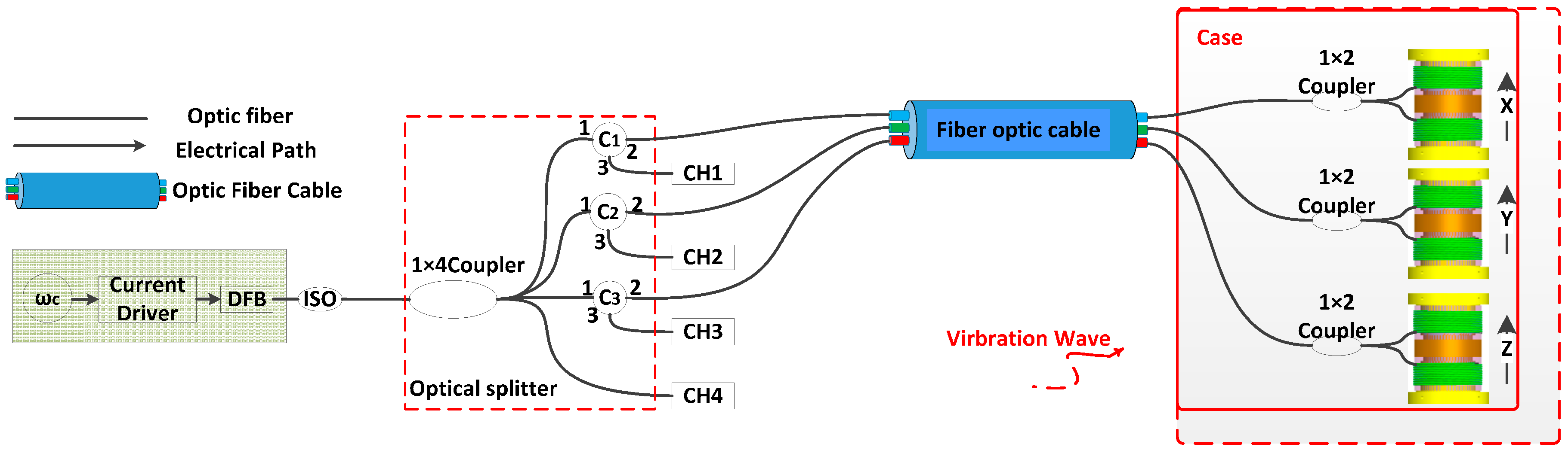
:1. Introduction
2. Demodulation Algorithm and Analysis for Accelerometer
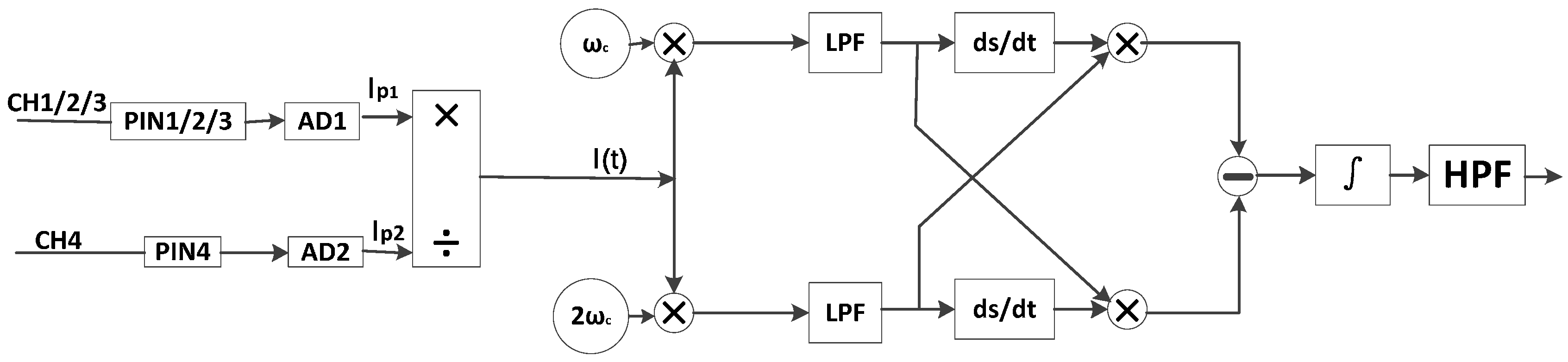
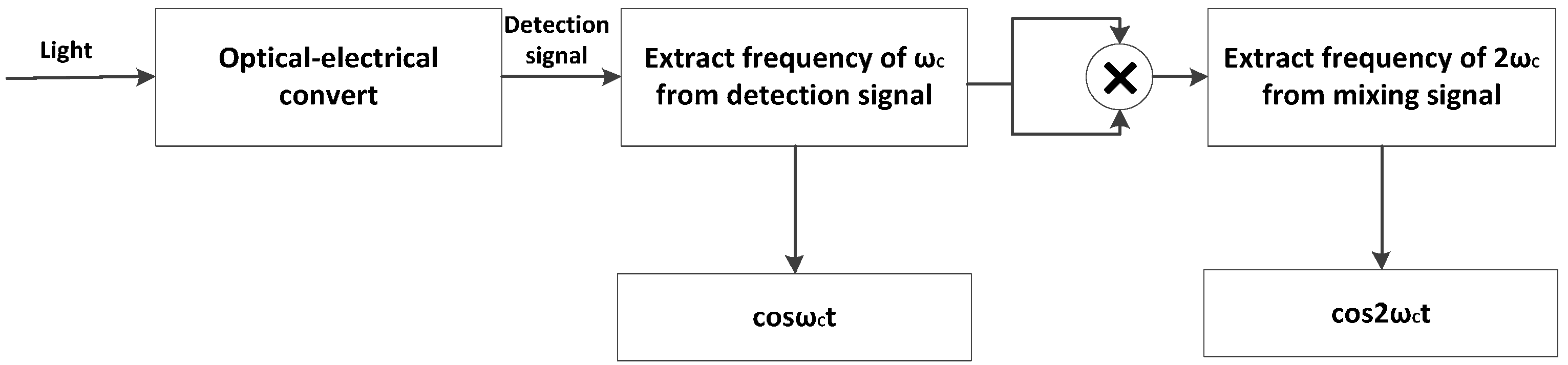
2.1. Demodulation of Direct Modulation Phase Generated Carrier
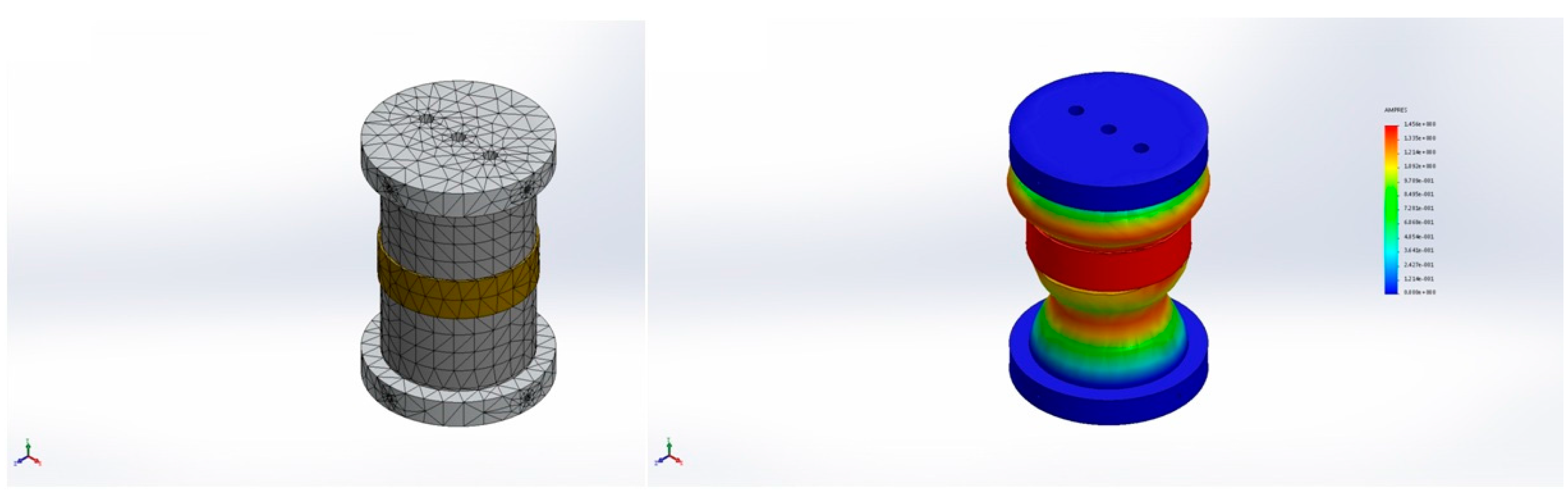
2.2. Design of Detector
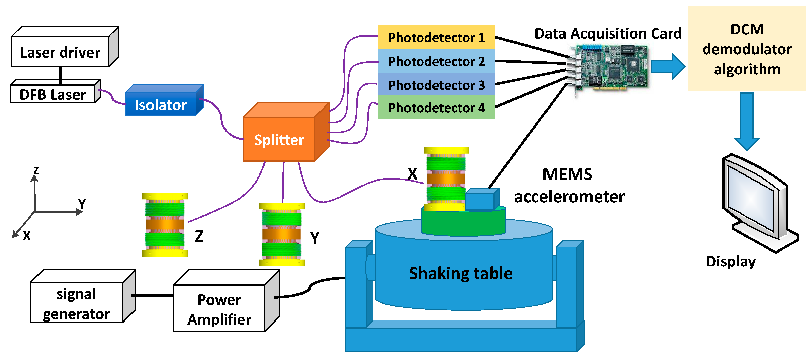
3. Experimental Results and Discussion
3.1. Responsivity and Operation Range of Frequency
3.2. Transverse Suppression Ratio
3.3. Minimum Detectable Signal Level and Dynamic Range
4. Conclusions
Acknowledgments
Author Contributions
Conflicts of Interest
References
- Rogers, G.C.; Meldrum, R.; Mulder, T.R.; Baldwin, R.; Rosenberger, A.; Moran, S.; Beeler, N.M. First observations form the NEPTUNE Canada seismograph network. Seismol. Res. Lett. 2010, 81, 369. [Google Scholar]
- Moran, K. Canada’s cabled ocean networks humming along. Eos Trans. Am. Geophys. Union 2013, 94, 17–19. [Google Scholar] [CrossRef]
- Cavill, A.W.; Cassidy, J.; Brennan, B.J. Results from the new seismic monitoring network at Egmont Volcano, New Zealand: Tectonic and hazard implications. N. Z. J. Geol. Geophys. 1997, 40, 69–76. [Google Scholar] [CrossRef]
- Okada, Y.; Kasahara, K.; Hori, S.; Obara, K.; Sekiguchi, S.; Fujiwara, H.; Yamamoto, A. Recent progress of seismic observation network in Japan. Earth Planets Space 2004, 56. [Google Scholar] [CrossRef]
- Cranch, G.A.; Nash, P.J.; Kirkendall, C.K. Large-Scale Remotely Interrogated Arrays of Fiber-optic Interferometric Sensors for Underwater Acoustic Applications. IEEE Sens. J. 2003, 3, 19–30. [Google Scholar] [CrossRef]
- Gulaev, A.Y.; Kitaev, S.M.; Listvin, V.N.; Potapov, V.T.; Sedykh, D.A.; Shatalin, S.V.; Yushkaĭtis, R.V. Deep-water fiber-optic hydrophone. Sov. J. Quantum Electron. 1990, 20, 867–868. [Google Scholar] [CrossRef]
- Kirkendall, C.K.; Dandridge, A. Overview of high performance fiber-optic sensing. J. Phys. D Appl. Phys. 2004, 37, R197–R216. [Google Scholar] [CrossRef]
- Shindo, Y.; Yoshikawa, T.; Mikada, H. A large scale seismic sensing array on the seafloor with fiber optic accelerometers. In Proceedings of the IEEE Sensors 2002, Orlando, FL, USA, 12–14 June 2002; Volume 2, pp. 1767–1770.
- Kersey, A.D.; Jackson, D.A.; Corke, M. High-sensitivity fiber-optic accelerometer. Electron. Lett. 1982, 18, 559. [Google Scholar] [CrossRef]
- Mills, G.B.; Garrett, S.L.; Carome, E.F. Fiber-optic gradient hydrophone. Tech. Symp. East 1984, 75, 98–103. [Google Scholar] [CrossRef]
- Gardner, D.L.; Hofler, T.; Baker, S.R.; Yarber, R.; Garrett, S. A fiber-optic interferometer seismometer. J. Light Technol. 1987, 5, 953–960. [Google Scholar] [CrossRef]
- Björn, N.P.P.; Toko, J.L.; Thornburg, J.A.; Slopko, F.; He, R.; Zhang, C.H. A high performance fiber optic seismic sensor system. In Proceedings of the Thirty-Eighth Workshop on Geothermal Reservoir Engineering Stanford University, Stanford, CA, USA, 11–13 February 2013.
- Brown, D.A.; Garrett, S.L. An interferometric fiber optic accelerometer. SPIE 1990, 1367, 282–288. [Google Scholar]
- Beverini, N.; Maccioni, E.; Morganti, M.; Stefani, F.; Falciai, R.; Trono, C. Fiber laser strain sensor device. J. Opt. A Pure Appl. Opt. 2007, 9, 958–962. [Google Scholar] [CrossRef]
- Wang, L.; He, J.; Lin, F.; Liu, Y. Ultra low frequency phase generated carrier demodulation technique for fiber sensors. Chin. J. Lasers 2011, 38. [Google Scholar] [CrossRef]
- Zeng, N.; Shi, C.Z.; Zhang, M.; Wang, L.W.; Liao, Y.B.; Lai, S.R. A 3-component fiber-optic accelerometer for well logging. Opt. Commun. 2004, 234, 153–162. [Google Scholar] [CrossRef]
- Jia, P.G.; Wang, D.H. Self-calibrated non-contact fibre-optic Fabry-Perot interferometric vibration displacement sensor system using laser emission frequency modulated phase generated carrier demodulation scheme. Meas. Sci. Technol. 2012, 23, 115201. [Google Scholar] [CrossRef]
- Shi, Q.; Tian, Q. Performance improvement of phase-generated carrier method by eliminating laser-intensity modulation for optical seismometer. Opt. Eng. 2010, 49, 024402. [Google Scholar]
- Tong, Y.; Zeng, H.; Li, L.; Zhou, Y. Improved phase generated carrier demodulation algorithm for eliminating light intensity disturbance and phase modulation amplitude variation. Appl. Opt. 2012, 51, 6962–6967. [Google Scholar] [CrossRef] [PubMed]
- Chen, Y.; Wang, J.; Luo, H.; Meng, Z. Research of the polarity characteristic for an optical fiber accelerometer demodulated by phase generated carrier technology. Optik 2014, 125, 3748–3751. [Google Scholar]
- He, J.; Wang, L.; Li, F.; Liu, Y. An ameliorated phase generated carrier demodulation algorithm with low harmonic distortion and high stability. J. Lightwave Technol. 2010, 28, 3258–3265. [Google Scholar]
- Huang, S.-C.; Huang, Y.-F.; Hwang, F.-H. An improved sensitivity normalization technique of PGC demodulation with low minimum phase detection sensitivity using laser modulation to generate carrier signal. Sens. Actuators A 2013, 191, 1–10. [Google Scholar] [CrossRef]
- Christian, T.R.; Frank, P.A.; Houston, B.H. Real-time analog and digital demodulator for interferometer fiber optic sensors. Proc. SPIE 1994, 2191, 324–326. [Google Scholar]
- Wang, Z.; Luo, H.; Xiong, S.; Ni, M.; Hu, Y. A J0-J1 method for measurement of dunamic phase changes in an interferometric fiber sensor. Chin. J. Lasers 2007, 34, 105–108. [Google Scholar]
- Shajenko, P.; Flatley, J.P.; Moffett, M.B. On fiber-optic hydrophone sensitivity. J. Acoust. Soc. Am. 1978, 64, 1286–1288. [Google Scholar] [CrossRef]
- Wang, Z.; Hu, Y.; Meng, Z.; Luo, H.; Ni, M. Novel mechanical antialiasing fiber-optic hydrophone with a fourth-order acoustic low-pass filter. Opt. Lett. 2008, 33, 1267–1269. [Google Scholar] [CrossRef] [PubMed]
- Yuan, W.; Pang, B.; Bo, J.; Qian, X. Fiber-optic sensor without polarization-induced signal fading. Microw. Opt. Technol. Lett. 2014, 56, 1307–1313. [Google Scholar] [CrossRef]
- De Freitas, J.M. Recent developments in seismic seabed oil reservoir nonitoring applications using fiber-optic sensing networks. Meas. Sci. Technol. 2011, 22, 052001. [Google Scholar] [CrossRef]


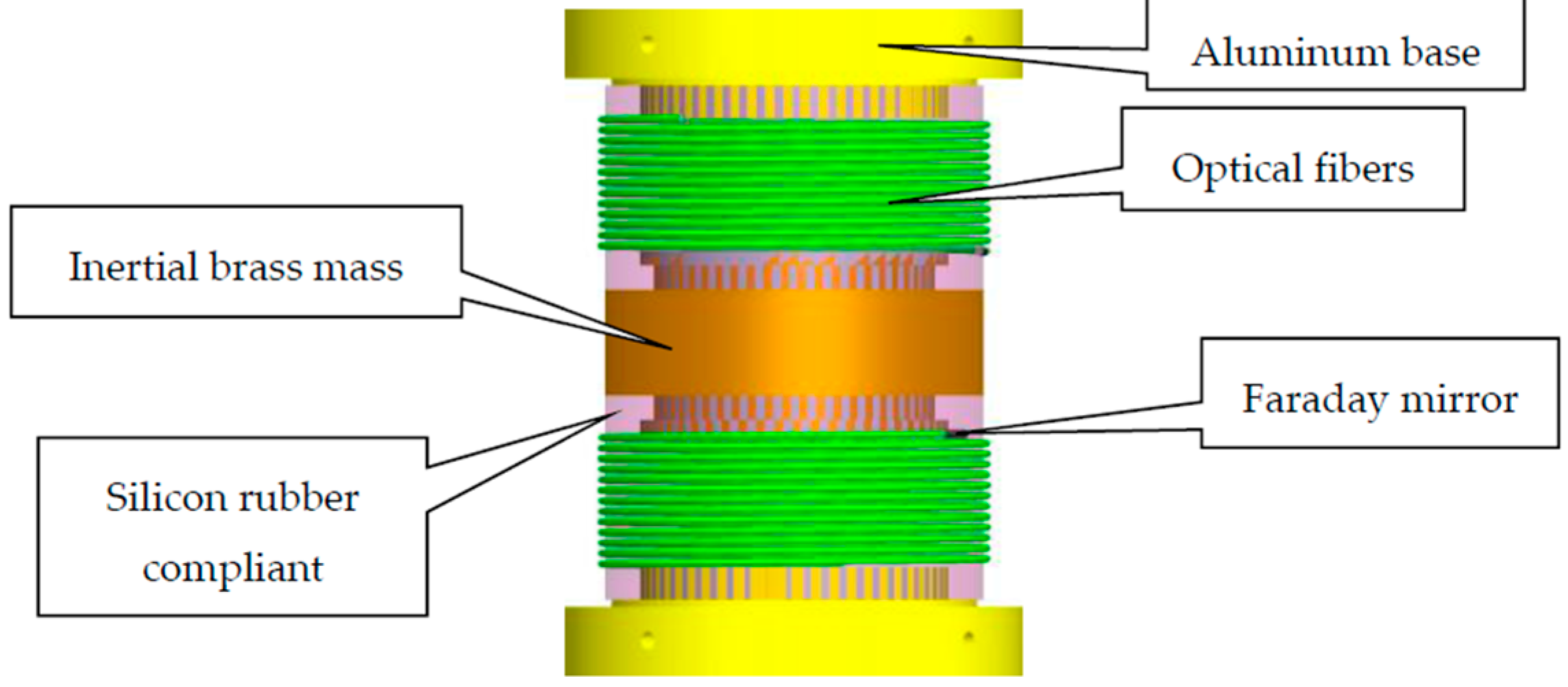
| Parts | Symbols | Parameters | Value (Units) |
|---|---|---|---|
| Inertial brass mass | ρ1 | Density | 8500 (kg/m3) |
| m1 | Mass | 412.5 (g) | |
| E1 | Young’s modulus | 1 × 10¹¹ (N/m2) | |
| δ1 | Poisson ratio | 0.33 | |
| Optical fibers | D2 | Diameter | 242 (um) |
| L2 | Length of fiber | 10 (m) | |
| E2 | Young’s modulus | 7.3 × 10¹⁰ (N/m2) | |
| δ2 | Poisson ratio | 0.17 | |
| Compliant cylinder | m3 | Mass | 59.0 (g) |
| ρ3 | Density | 1246.5 (kg/m3) | |
| E3 | Young’s modulus | 1.55 × 10⁶ (N/m2) | |
| δ3 | Poisson ratio | 0.48 | |
| δb | Tensile strength | 6 × 10⁶ (N/m2) | |
| Aluminum base | ρ4 | Density | 2700 (kg/m3) |
| m4 | Mass | 110.1 (g) | |
| E4 | Young’s modulus | 6.9 × 10¹⁰ (N/m2) | |
| δ4 | Poisson ratio | 0.33 |
| Model | The Average of the Transverse Suppression (2–150 Hz) | Transverse Suppression Ratio at 10 Hz |
|---|---|---|
| X | 32.64 dB | 34.61 dB |
| Y | 29.76 dB | 32.20 dB |
| Z | 28.57 dB | 30.77 dB |
| Model | The Minimum Detectable Acceleration |
|---|---|
| X | |
| Y | |
| Z |
© 2016 by the authors; licensee MDPI, Basel, Switzerland. This article is an open access article distributed under the terms and conditions of the Creative Commons Attribution (CC-BY) license (http://creativecommons.org/licenses/by/4.0/).
Share and Cite
Chen, J.; Chang, T.; Fu, Q.; Lang, J.; Gao, W.; Wang, Z.; Yu, M.; Zhang, Y.; Cui, H.-L. A Fiber-Optic Interferometric Tri-Component Geophone for Ocean Floor Seismic Monitoring. Sensors 2017, 17, 47. https://doi.org/10.3390/s17010047
Chen J, Chang T, Fu Q, Lang J, Gao W, Wang Z, Yu M, Zhang Y, Cui H-L. A Fiber-Optic Interferometric Tri-Component Geophone for Ocean Floor Seismic Monitoring. Sensors. 2017; 17(1):47. https://doi.org/10.3390/s17010047
Chicago/Turabian StyleChen, Jiandong, Tianying Chang, Qunjian Fu, Jinpeng Lang, Wenzhi Gao, Zhongmin Wang, Miao Yu, Yanbo Zhang, and Hong-Liang Cui. 2017. "A Fiber-Optic Interferometric Tri-Component Geophone for Ocean Floor Seismic Monitoring" Sensors 17, no. 1: 47. https://doi.org/10.3390/s17010047