
Depth Errors Analysis and Correction for Time-of-Flight (ToF) Cameras


Abstract
:1. Introduction
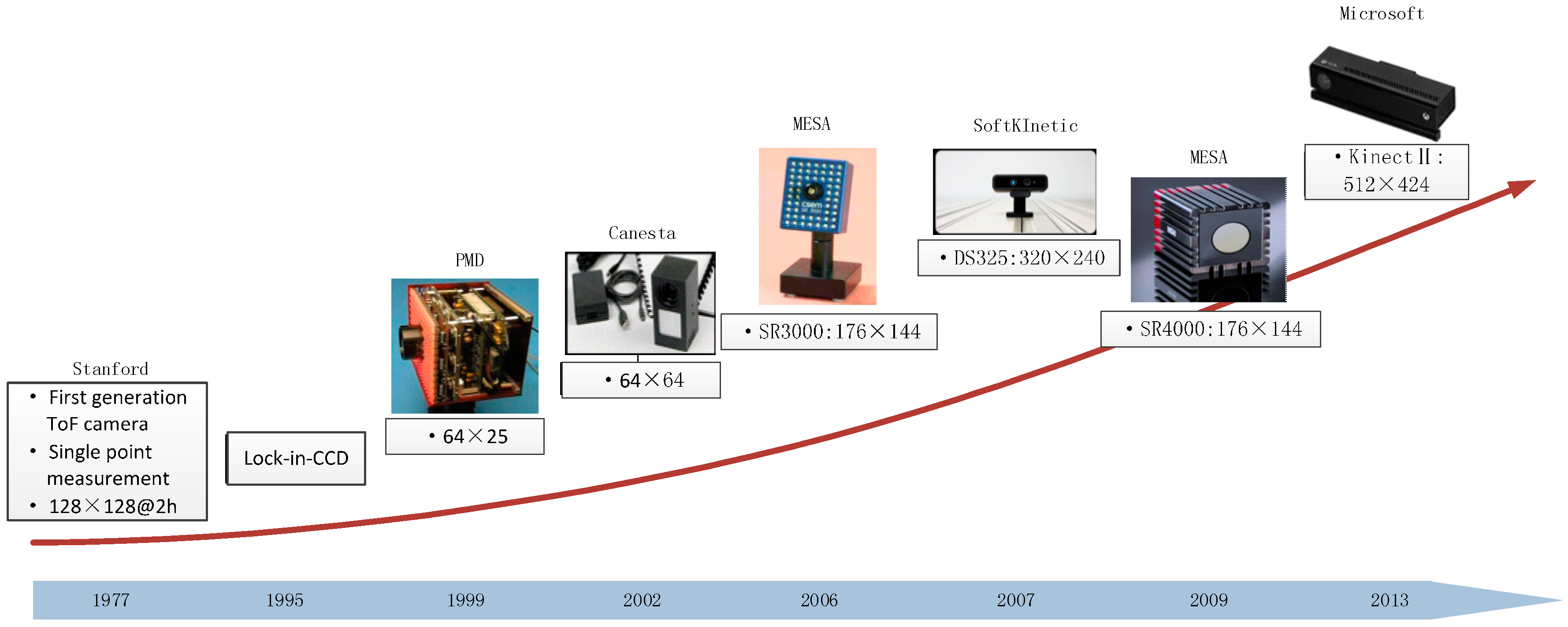
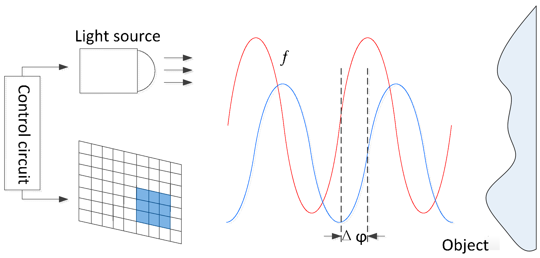
2. Development and Principle of ToF Cameras
3. Analysis on Depth Errors of ToF Cameras
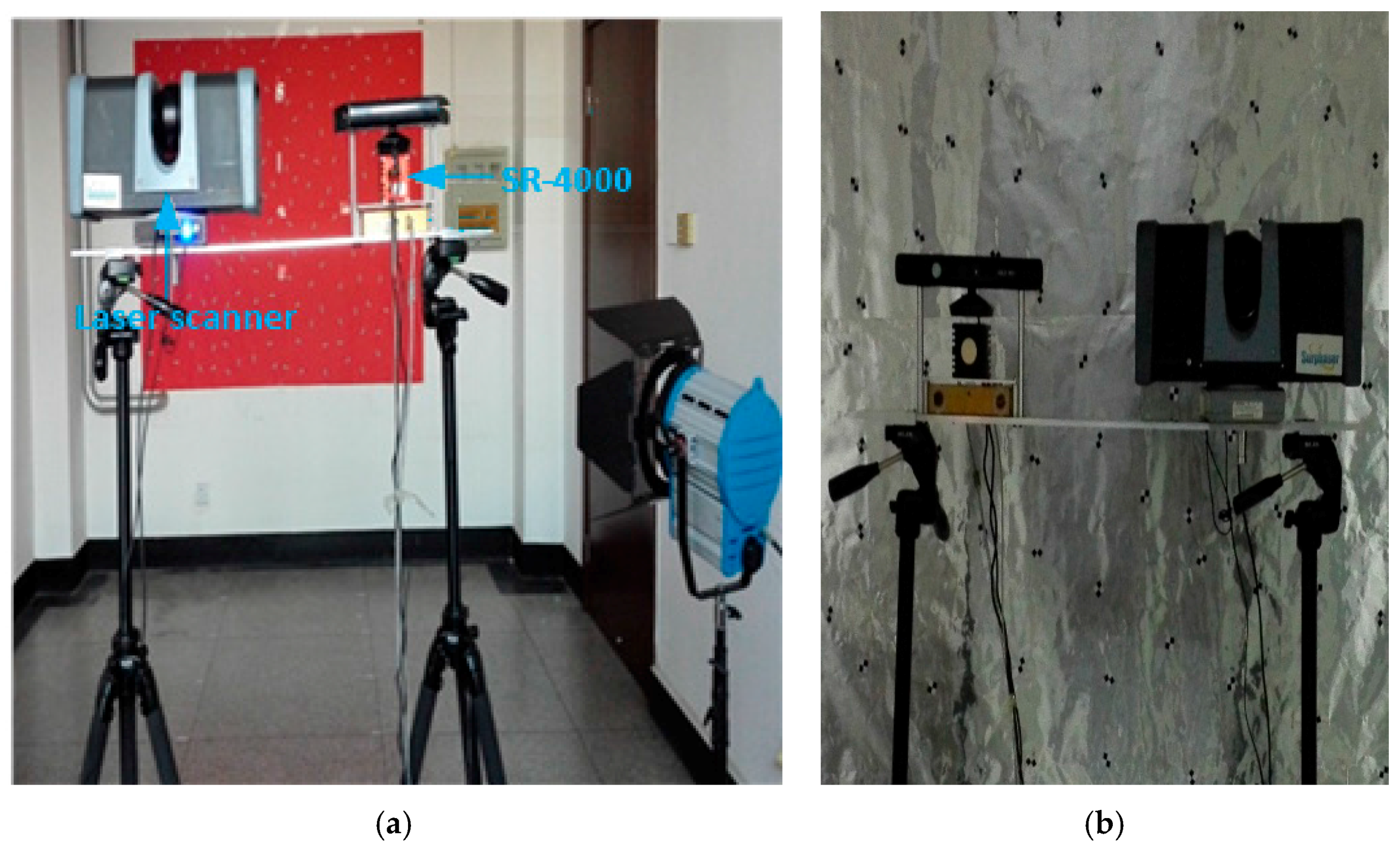
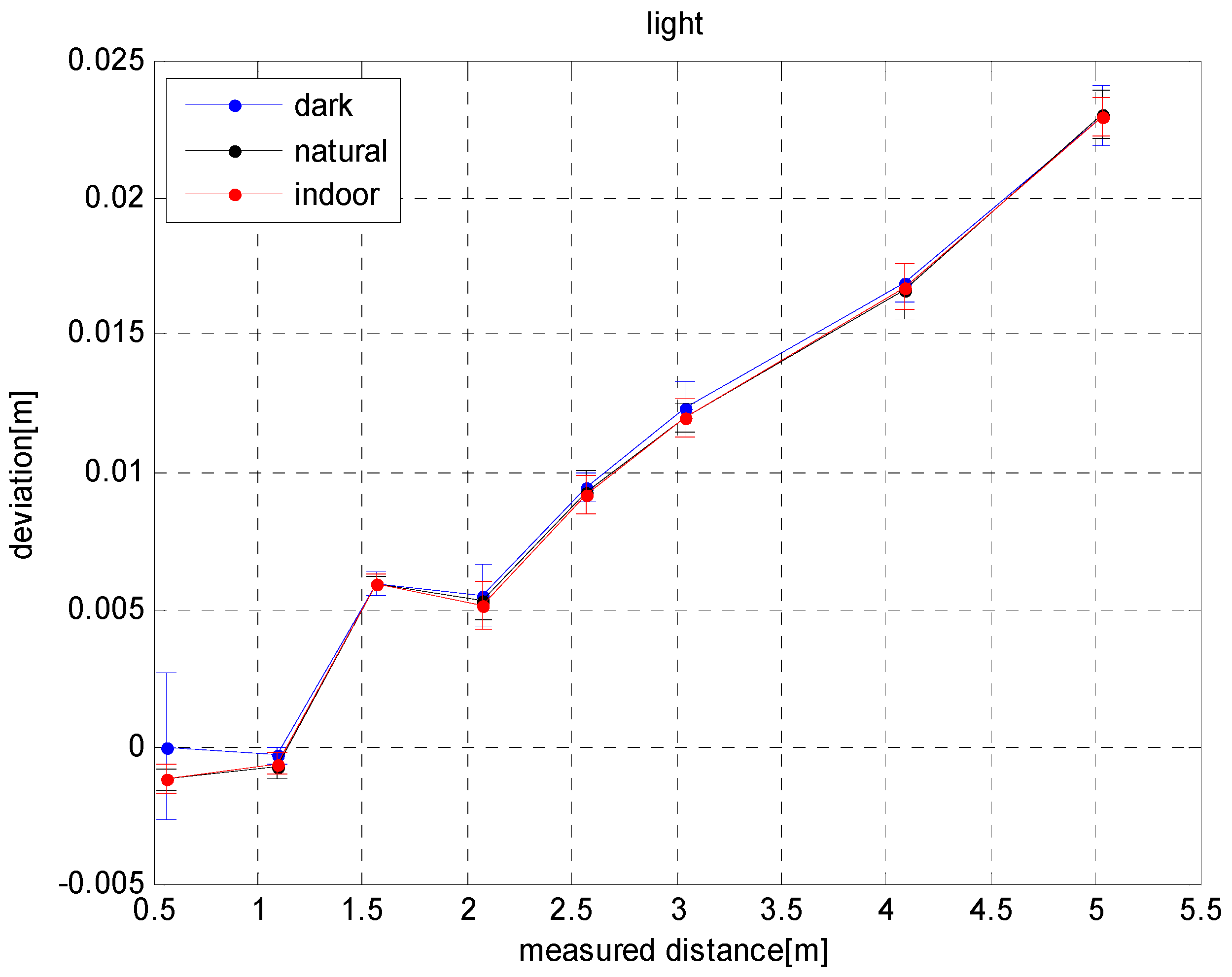
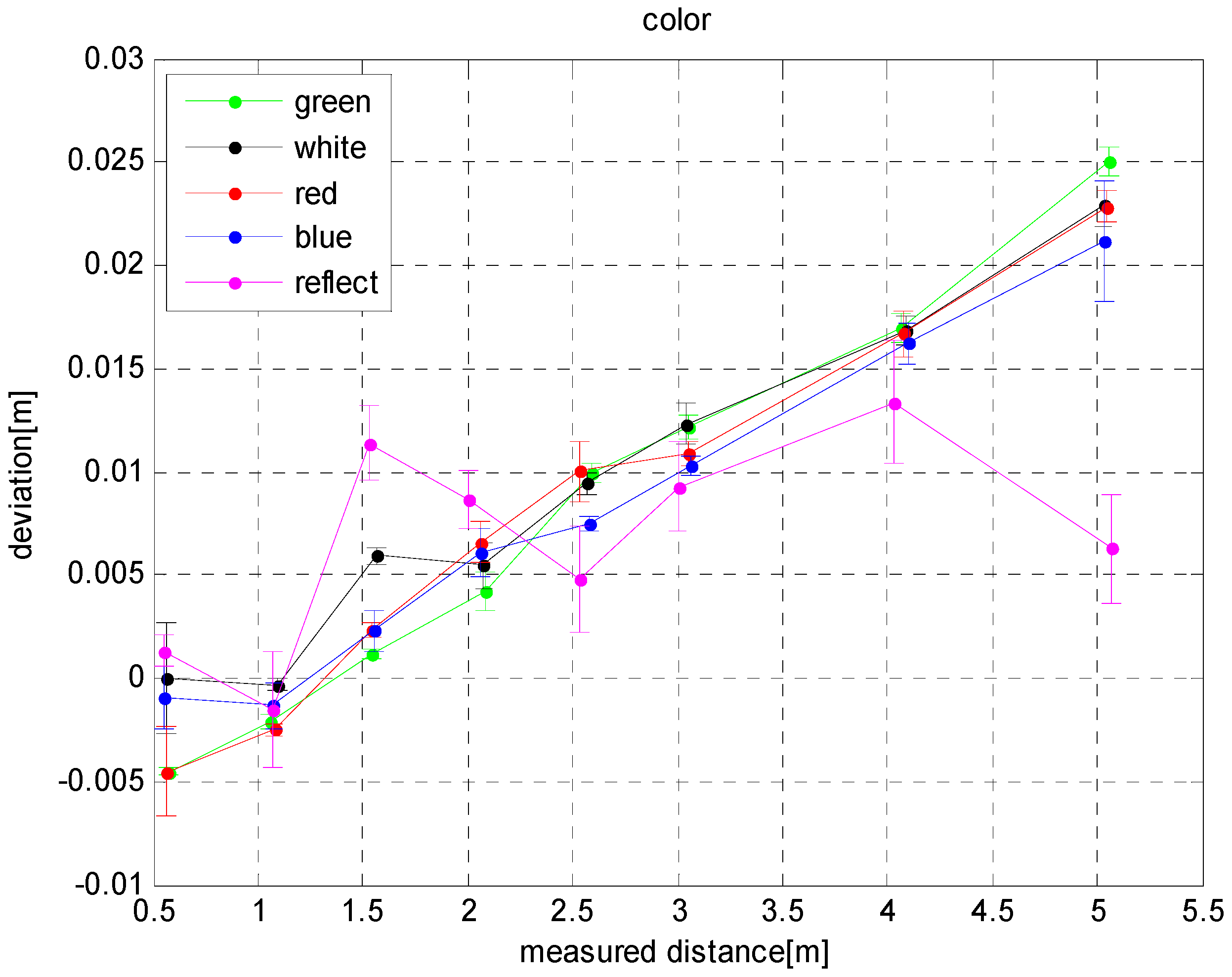
3.1. Influence of Lighting, Color and Distance on Depth Errors
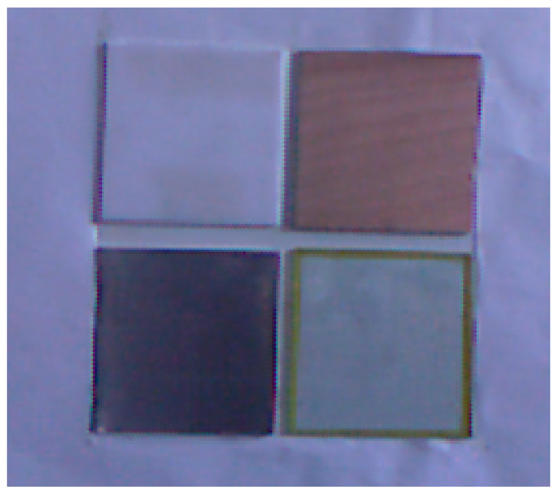
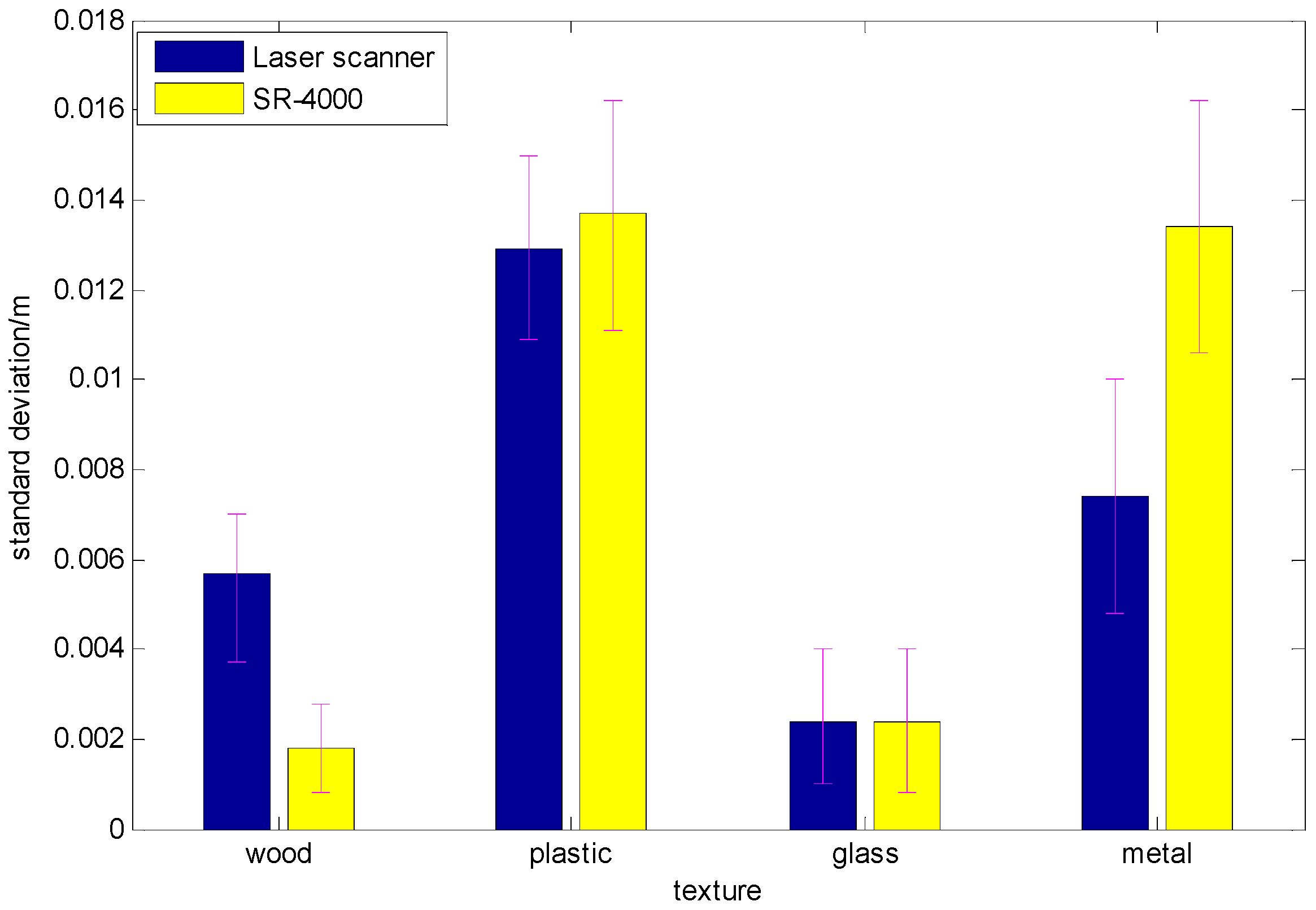
3.2. Influence of Material on Depth Errors
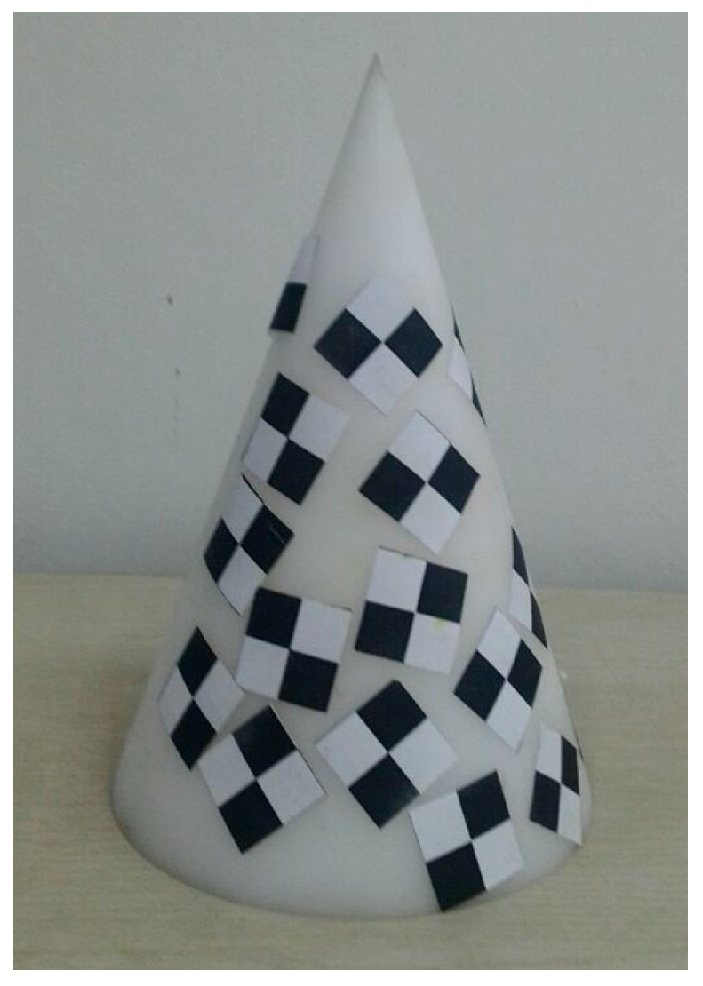
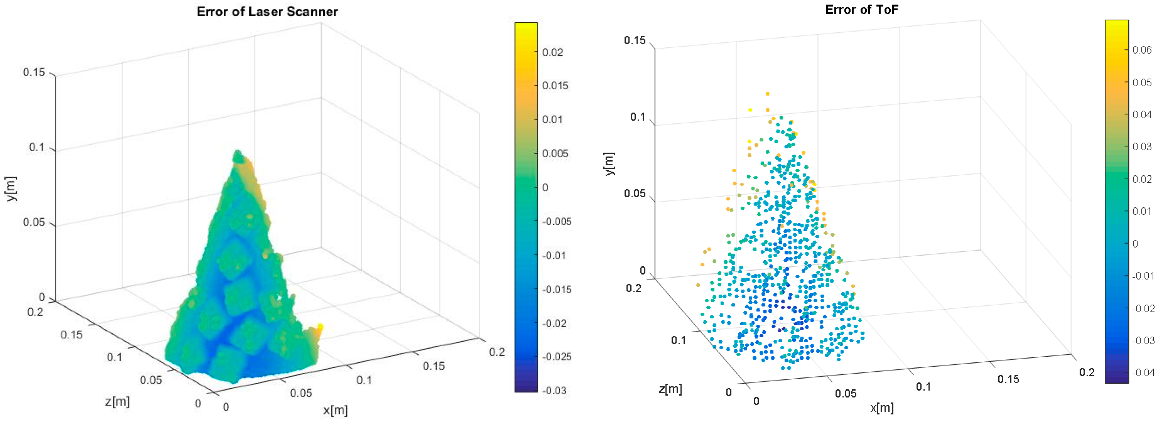
3.3. Influence of a Single Scene on Depth Errors
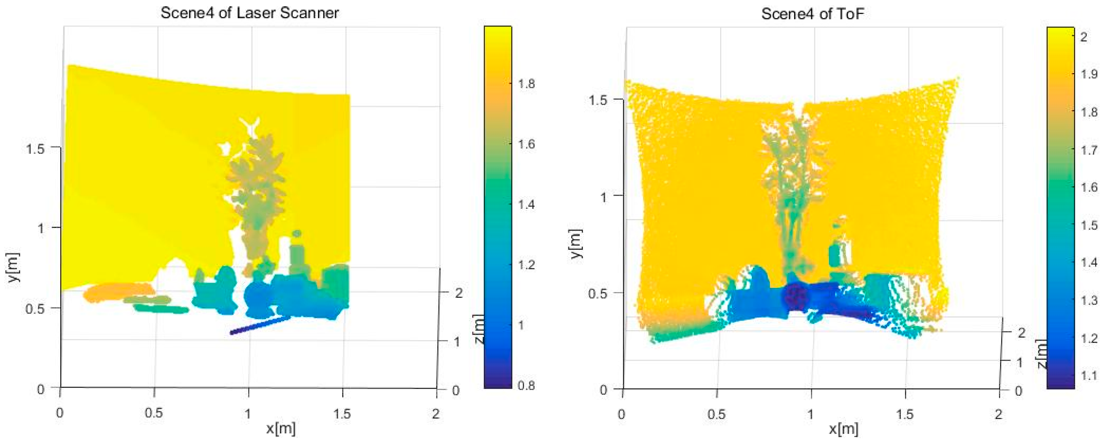
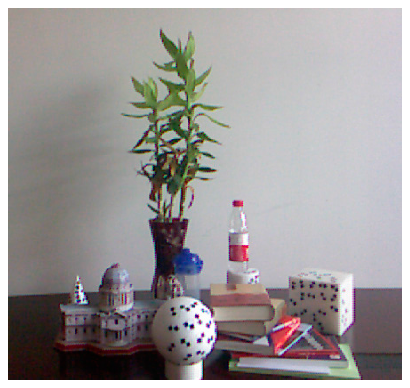
3.4. Influence of a Complex Scene on Depth Errors
3.5. Analysis of Depth Errors
4. Depth Error Correction for ToF Cameras
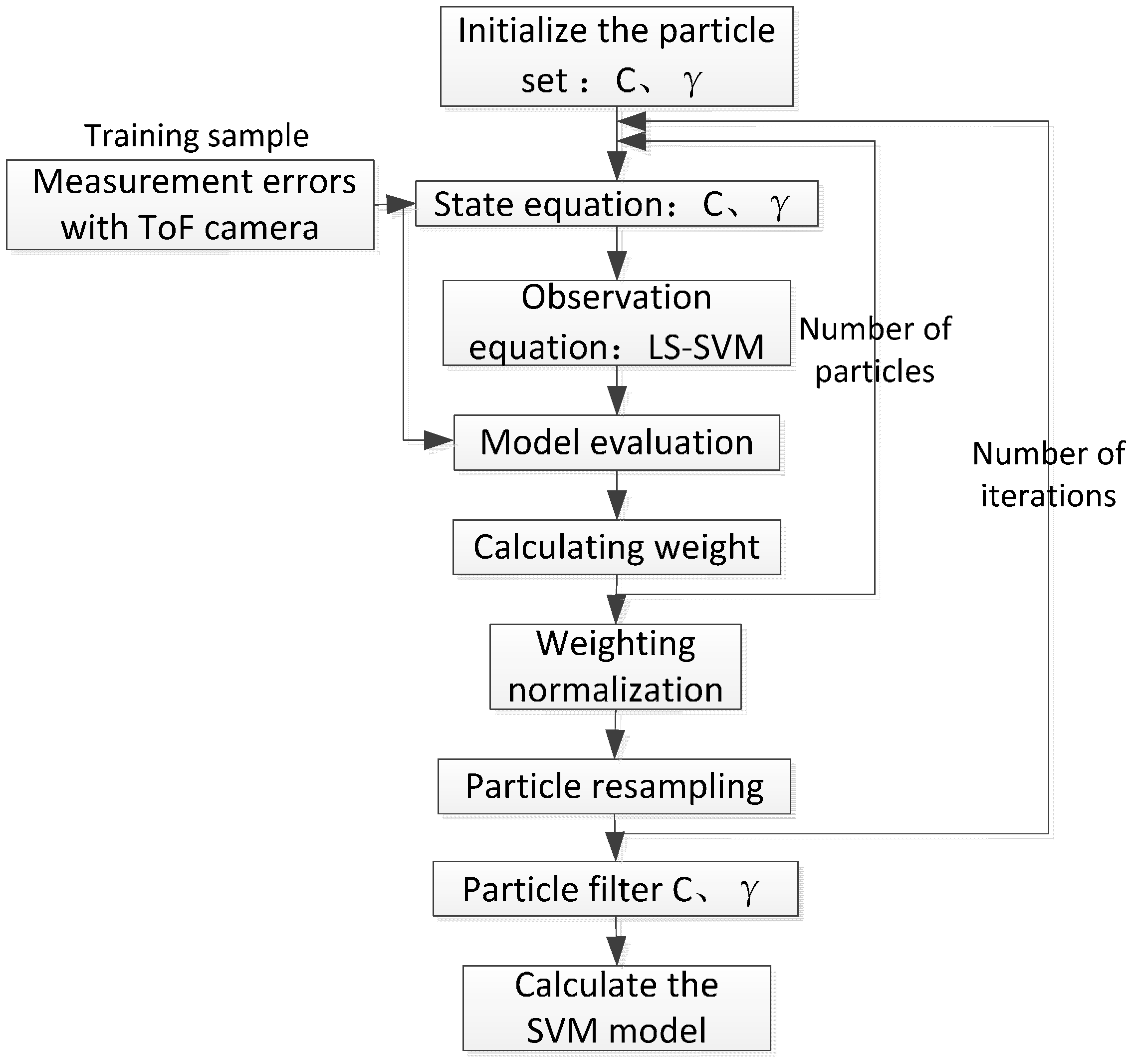
4.1. PF-SVM Algorithm
4.1.1. LS-SVM Algorithm
4.1.2. PF-SVM Algorithm
4.2. Experimental Results
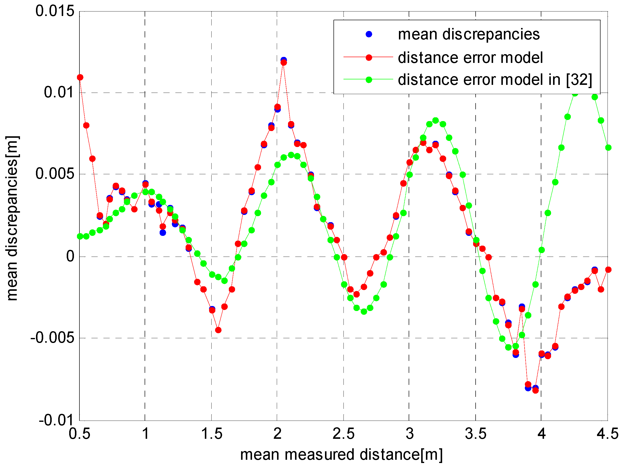
4.2.1. Experiment 1
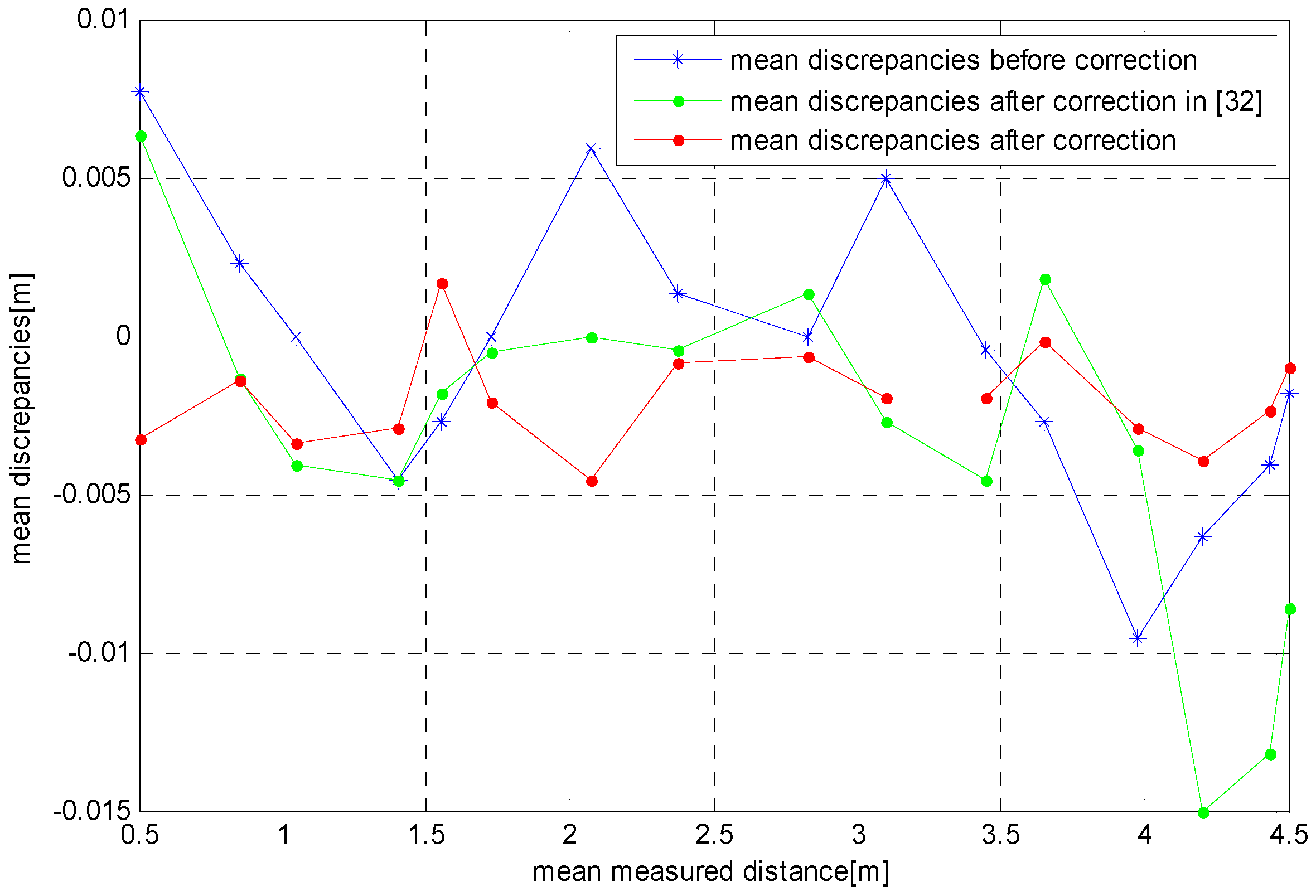
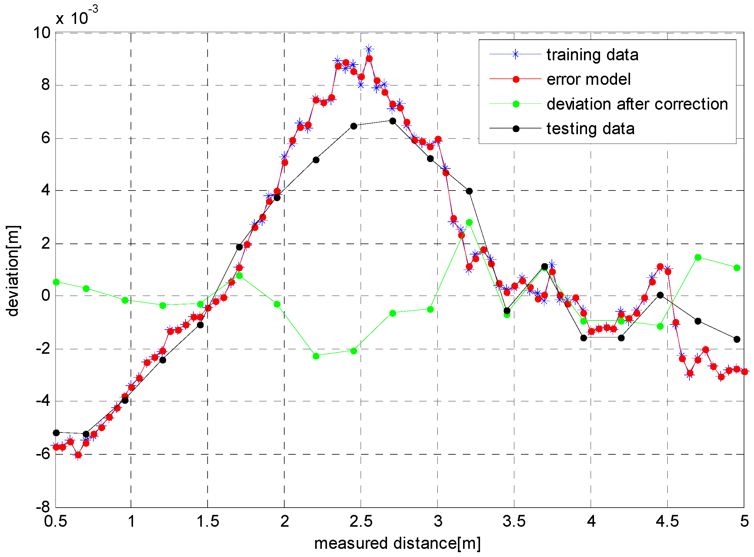
4.2.2. Experiment 2
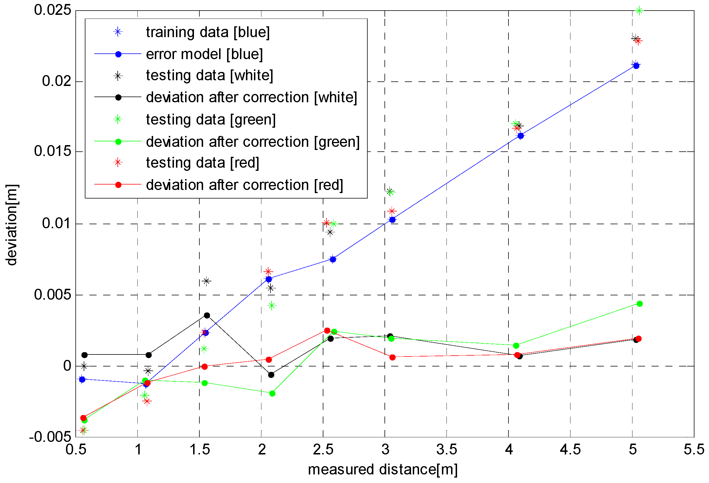
4.2.3. Experiment 3
5. Conclusions
Acknowledgments
Author Contributions
Conflicts of Interest
References
- Henry, P.; Krainin, M.; Herbst, E.; Ren, X.; Fox, D. RGB-D mapping: Using kinect-style depth cameras for dense 3D modeling of indoor environments. Int. J. Robot. Res. 2012, 31, 647–663. [Google Scholar] [CrossRef]
- Brachmann, E.; Krull, A.; Michel, F.; Gumhold, S.; Shotton, J.; Rother, C. Learning 6D Object Pose Estimation Using 3D Object Coordinates; Springer: Heidelberg, Germany, 2014; Volume 53, pp. 151–173. [Google Scholar]
- Tong, J.; Zhou, J.; Liu, L.; Pan, Z.; Yan, H. Scanning 3D full human bodies using kinects. IEEE Trans. Vis. Comput. Graph. 2012, 18, 643–650. [Google Scholar] [CrossRef] [PubMed]
- Liu, X.; Fujimura, K. Hand gesture recognition using depth data. In Proceedings of the IEEE International Conference on Automatic Face and Gesture Recognition, Seoul, Korea, 17–19 May 2004; pp. 529–534.
- Foix, S.; Alenya, G.; Torras, C. Lock-in time-of-flight (ToF) cameras: A survey. IEEE Sens. J. 2011, 11, 1917–1926. [Google Scholar] [CrossRef] [Green Version]
- Wiedemann, M.; Sauer, M.; Driewer, F.; Schilling, K. Analysis and characterization of the PMD camera for application in mobile robotics. IFAC Proc. Vol. 2008, 41, 13689–13694. [Google Scholar] [CrossRef]
- Fuchs, S.; May, S. Calibration and registration for precise surface reconstruction with time of flight cameras. Int. J. Int. Syst. Technol. App. 2008, 5, 274–284. [Google Scholar] [CrossRef]
- Guomundsson, S.A.; Aanæs, H.; Larsen, R. Environmental effects on measurement uncertainties of time-of-flight cameras. In Proceedings of the 2007 International Symposium on Signals, Circuits and Systems, Iasi, Romania, 12–13 July 2007; Volumes 1–2, pp. 113–116.
- Rapp, H. Experimental and Theoretical Investigation of Correlating ToF-Camera Systems. Master’s Thesis, University of Heidelberg, Heidelberg, Germany, September 2007. [Google Scholar]
- Falie, D.; Buzuloiu, V. Noise characteristics of 3D time-of-flight cameras. In Proceedings of the 2007 International Symposium on Signals, Circuits and Systems, Iasi, Romania, 12–13 July 2007; Volumes 1–2, pp. 229–232.
- Karel, W.; Dorninger, P.; Pfeifer, N. In situ determination of range camera quality parameters by segmentation. In Proceedings of the VIII International Conference on Optical 3-D Measurement Techniques, Zurich, Switzerland, 9–12 July 2007; pp. 109–116.
- Kahlmann, T.; Ingensand, H. Calibration and development for increased accuracy of 3D range imaging cameras. J. Appl. Geodesy 2008, 2, 1–11. [Google Scholar] [CrossRef]
- Karel, W. Integrated range camera calibration using image sequences from hand-held operation. Int. Arch. Photogramm. Remote Sens. Spat. Inf. Sci. 2008, 37, 945–952. [Google Scholar]
- May, S.; Werner, B.; Surmann, H.; Pervolz, K. 3D time-of-flight cameras for mobile robotics. In Proceedings of the 2006 IEEE/RSJ International Conference on Intelligent Robots and Systems, Beijing, China, 9–15 October 2006; Volumes 1–12, pp. 790–795.
- Kirmani, A.; Benedetti, A.; Chou, P.A. Spumic: Simultaneous phase unwrapping and multipath interference cancellation in time-of-flight cameras using spectral methods. In Proceedings of the IEEE International Conference on Multimedia and Expo (ICME), San Jose, CA, USA, 15–19 July 2013; pp. 1–6.
- Freedman, D.; Krupka, E.; Smolin, Y.; Leichter, I.; Schmidt, M. Sra: Fast removal of general multipath for ToF sensors. In Proceedings of the European Conference on Computer Vision, Zurich, Switzerland, 6–12 September 2014.
- Kadambi, A.; Whyte, R.; Bhandari, A.; Streeter, L.; Barsi, C.; Dorrington, A.; Raskar, R. Coded time of flight cameras: Sparse deconvolution to address multipath interference and recover time profiles. ACM Trans. Graph. 2013, 32, 167. [Google Scholar] [CrossRef]
- Whyte, R.; Streeter, L.; Gree, M.J.; Dorrington, A.A. Resolving multiple propagation paths in time of flight range cameras using direct and global separation methods. Opt. Eng. 2015, 54, 113109. [Google Scholar] [CrossRef] [Green Version]
- Lottner, O.; Sluiter, A.; Hartmann, K.; Weihs, W. Movement artefacts in range images of time-of-flight cameras. In Proceedings of the 2007 International Symposium on Signals, Circuits and Systems, Iasi, Romania, 13–14 July 2007; Volumes 1–2, pp. 117–120.
- Lindner, M.; Kolb, A. Compensation of motion artifacts for time-of flight cameras. In Dynamic 3D Imaging; Springer: Heidelberg, Germany, 2009; Volume 5742, pp. 16–27. [Google Scholar]
- Lee, S.; Kang, B.; Kim, J.D.K.; Kim, C.Y. Motion Blur-free time-of-flight range sensor. Proc. SPIE 2012, 8298, 105–118. [Google Scholar]
- Lee, C.; Kim, S.Y.; Kwon, Y.M. Depth error compensation for camera fusion system. Opt. Eng. 2013, 52, 55–68. [Google Scholar] [CrossRef]
- Kuznetsova, A.; Rosenhahn, B. On calibration of a low-cost time-of-flight camera. In Proceedings of the Workshop at the European Conference on Computer Vision, Zurich, Switzerland, 6–12 September 2014; Lecture Notes in Computer Science. Volume 8925, pp. 415–427.
- Lee, S. Time-of-flight depth camera accuracy enhancement. Opt. Eng. 2012, 51, 527–529. [Google Scholar] [CrossRef]
- Christian, J.A.; Cryan, S. A survey of LIDAR technology and its use in spacecraft relative navigation. In Proceedings of the AIAA Guidance, Navigation, and Control Conference, Boston, MA, USA, 19–22 August 2013; pp. 1–7.
- Nitzan, D.; Brain, A.E.; Duda, R.O. Measurement and use of registered reflectance and range data in scene analysis. Proc. IEEE 1977, 65, 206–220. [Google Scholar] [CrossRef]
- Spirig, T.; Seitz, P.; Vietze, O. The lock-in CCD 2-dimensional synchronous detection of light. IEEE J. Quantum Electron. 1995, 31, 1705–1708. [Google Scholar] [CrossRef]
- Schwarte, R. Verfahren und vorrichtung zur bestimmung der phasen-und/oder amplitude information einer elektromagnetischen Welle. DE Patent 19,704,496, 12 March 1998. [Google Scholar]
- Lange, R.; Seitz, P.; Biber, A.; Schwarte, R. Time-of-flight range imaging with a custom solid-state image sensor. Laser Metrol. Inspect. 1999, 3823, 180–191. [Google Scholar]
- Piatti, D.; Rinaudo, F. SR-4000 and CamCube3.0 time of flight (ToF) cameras: Tests and comparison. Remote Sens. 2012, 4, 1069–1089. [Google Scholar] [CrossRef]
- Chiabrando, F.; Piatti, D.; Rinaudo, F. SR-4000 ToF camera: Further experimental tests and first applications to metric surveys. Int. Arch. Photogramm. Remote Sens. Spat. Inf. Sci. 2010, 38, 149–154. [Google Scholar]
- Chiabrando, F.; Chiabrando, R.; Piatti, D. Sensors for 3D imaging: Metric evaluation and calibration of a CCD/CMOS time-of-flight camera. Sensors 2009, 9, 10080–10096. [Google Scholar] [CrossRef] [PubMed]
- Charleston, S.A.; Dorrington, A.A.; Streeter, L.; Cree, M.J. Extracting the MESA SR4000 calibrations. In Proceedings of the Videometrics, Range Imaging, and Applications XIII, Munich, Germany, 22–25 June 2015; Volume 9528.
- Ye, C.; Bruch, M. A visual odometry method based on the SwissRanger SR4000. Proc. SPIE 2010, 7692, 76921I. [Google Scholar]
- Hong, S.; Ye, C.; Bruch, M.; Halterman, R. Performance evaluation of a pose estimation method based on the SwissRanger SR4000. In Proceedings of the IEEE International Conference on Mechatronics and Automation, Chengdu, China, 5–8 August 2012; pp. 499–504.
- Lahamy, H.; Lichti, D.; Ahmed, T.; Ferber, R.; Hettinga, B.; Chan, T. Marker-less human motion analysis using multiple Sr4000 range cameras. In Proceedings of the 13th International Symposium on 3D Analysis of Human Movement, Lausanne, Switzerland, 14–17 July 2014.
- Kahlmann, T.; Remondino, F.; Ingensand, H. Calibration for increased accuracy of the range imaging camera SwissrangerTM. In Proceedings of the ISPRS Commission V Symposium Image Engineering and Vision Metrology, Dresden, Germany, 25–27 September 2006; pp. 136–141.
- Weyer, C.A.; Bae, K.; Lim, K.; Lichti, D. Extensive metric performance evaluation of a 3D range camera. Int. Soc. Photogramm. Remote Sens. 2008, 37, 939–944. [Google Scholar]
- Mure-Dubois, J.; Hugli, H. Real-Time scattering compensation for time-of-flight camera. In Proceedings of the ICVS Workshop on Camera Calibration Methods for Computer Vision Systems, Bielefeld, Germany, 21–24 March 2007.
- Kavli, T.; Kirkhus, T.; Thielmann, J.; Jagielski, B. Modeling and compensating measurement errors caused by scattering time-of-flight cameras. In Proceedings of the SPIE, Two-and Three-Dimensional Methods for Inspection and Metrology VI, San Diego, CA, USA, 10 August 2008.
- Vapnik, V.N. The Nature of Statistical Learning Theory; Springer: New York, NY, USA, 1995. [Google Scholar]
- Ales, J.S.; Bernhand, S. A tutorialon support vector regression. Stat. Comput. 2004, 14, 199–222. [Google Scholar]
- Suykens, J.A.K.; Vandewalle, J. Least squares support vector machine classifiers. Neural Process. Lett. 1999, 9, 293–300. [Google Scholar] [CrossRef]
- Zhang, J.; Wang, S. A fast leave-one-out cross-validation for SVM-like family. Neural Comput. Appl. 2016, 27, 1717–1730. [Google Scholar] [CrossRef]
- Gustafsson, F. Particle filter theory and practice with positioning applications. IEEE Aerosp. Electron. Syst. Mag. 2010, 25, 53–82. [Google Scholar] [CrossRef]


| ToF Camera | Maximum Resolution of Depth Images | Maximum Frame Rate/fps | Measurement Rage/m | Field of View/° | Accuracy | Weight/g | Power/W (Typical/Maximum) | |
|---|---|---|---|---|---|---|---|---|
| MESA-SR4000 |  | 176 × 144 | 50 | 0.1–5 | 69 × 55 | ±1 cm | 470 | 9.6/24 |
| Microsoft-Kinect II |  | 512 × 424 | 30 | 0.5–4.5 | 70 × 60 | ±3 cm@2 m | 550 | 16/32 |
| PMD-Camcube 3.0 |  | 200 × 200 | 15 | 0.3–7.5 | 40 × 40 | ±3 mm@4 m | 1438 | - |
| Comparison Items | Maximal Error/mm | Average Error/mm | Variance/mm | Optimal Range/m | Running Time/s | |||
|---|---|---|---|---|---|---|---|---|
| 1.5–4 | 0.5–4.5 | 1.5–4 | 0.5–4.5 | 1.5–4 | 0.5–4.5 | |||
| This paper’s algorithm | 4.6 | 4.6 | 1.99 | 2.19 | 2.92 | 2.4518 | 0.5–4.5 | 2 |
| Reference [32] algorithm | 4.6 | 8.6 | 2.14 | 4.375 | 5.34 | 29.414 | 1.5–4 | - |
© 2017 by the authors; licensee MDPI, Basel, Switzerland. This article is an open access article distributed under the terms and conditions of the Creative Commons Attribution (CC-BY) license (http://creativecommons.org/licenses/by/4.0/).
Share and Cite
He, Y.; Liang, B.; Zou, Y.; He, J.; Yang, J. Depth Errors Analysis and Correction for Time-of-Flight (ToF) Cameras. Sensors 2017, 17, 92. https://doi.org/10.3390/s17010092
He Y, Liang B, Zou Y, He J, Yang J. Depth Errors Analysis and Correction for Time-of-Flight (ToF) Cameras. Sensors. 2017; 17(1):92. https://doi.org/10.3390/s17010092
Chicago/Turabian StyleHe, Ying, Bin Liang, Yu Zou, Jin He, and Jun Yang. 2017. "Depth Errors Analysis and Correction for Time-of-Flight (ToF) Cameras" Sensors 17, no. 1: 92. https://doi.org/10.3390/s17010092