A Weighted Measurement Fusion Particle Filter for Nonlinear Multisensory Systems Based on Gauss–Hermite Approximation


1
School of Electronic Engineering, Heilongjiang University, Harbin 150080, China
2
School of Computer and Information Engineering, Harbin University of Commerce, Harbin 150001, China
*
Author to whom correspondence should be addressed.
Sensors 2017, 17(10), 2222; https://doi.org/10.3390/s17102222
Submission received: 8 August 2017
/
Revised: 24 September 2017
/
Accepted: 26 September 2017
/
Published: 28 September 2017
(This article belongs to the Special Issue Advances in Multi-Sensor Information Fusion: Theory and Applications 2017)
Abstract
:We addressed the fusion estimation problem for nonlinear multisensory systems. Based on the Gauss–Hermite approximation and weighted least square criterion, an augmented high-dimension measurement from all sensors was compressed into a lower dimension. By combining the low-dimension measurement function with the particle filter (PF), a weighted measurement fusion PF (WMF-PF) is presented. The accuracy of WMF-PF appears good and has a lower computational cost when compared to centralized fusion PF (CF-PF). An example is given to show the effectiveness of the proposed algorithms.
1. Introduction
State estimation algorithms play an important part in automatic control, target tracking, navigation, fault diagnosis, and so on. However, it is difficult for single sensor to obtain accurate estimation and good fault tolerance, so multisensory fusion estimation technology was created to overcome this issue. There are two main kinds of fundamental estimation fusion structures: centralized fusion and distributed fusion. Centralized fusion combines measurements of all sensors into an augmented measurement, and then the data processing center outputs the fused state estimate. The advantage of centralized fusion is that there is no information loss and is ideal when all sensors are fully functional, so it is used as a comparative standard for other fusion algorithms. However, with a large number of sensors, the centralized fusion algorithm performs poorly in real time and is not reliable because of expensive computation due to augmented high-dimension measurements. In the sensor network, a large number of different types of sensors exist. If the data from the sensors are processed in a centralized way, the computational cost will be high. Especially in wireless sensor networks, large amounts of data from nodes make it difficult for decision centers to make timely decisions. In such cases, data compression must be used, and weighted measurement fusion (WMF) is one of these data compression methods [1,2,3].
Distributed fusion algorithms produce a fused estimate by combining local state estimates under a certain criterion in the fusion center [4,5,6,7]. Distributed fusion algorithms, such as the distributed fusion federated Kalman filter [8], the distributed weighted fusion estimation [9], and the distributed covariance intersection (CI) fusion estimation [10], are robust and flexible because of their parallel computing structures [3]. They are optimal for local application but are suboptimal for global use, as their accuracy is lower than the centralized fusion algorithm. WMF algorithms compress a high-dimension measurement to a low-dimension measurement under certain criterion [11,12,13], so the computational cost can be reduced when implementing particle filter (PF) based on the compressed measurement. For linear systems, the WMF algorithms are equivalent to centralized fusion [11,13], so they are also optimal in terms of least mean squares. In this paper, the WMF method will be studied given the abovementioned advantages.
Estimation fusion has formed a complete theory for linear systems over the past years. However, most systems have nonlinear parts. For example, the measurement functions, in sensor models, of most tracking systems are established under spherical coordinates, and are strongly nonlinear when the states are estimated under Cartesian coordinates [14,15]. For nonlinear systems, fusion algorithms, which are achieved by the Taylor series, based on the Extended Kalman filter (EKF) are commonly used [16,17,18,19]. These algorithms are simple since they can be converted into linear systems. However, they result in large estimation bias and even lead to filtering divergence due to the amount of information being omitted. Many nonlinear fusion approaches have been presented, including random set, artificial neural networks, fuzzy logic, rough set, dempster-shafer, and other non-probabilistic approaches [20,21]. These methods fuse information and compress data. Given the amount of information lost, they are usually suboptimal.
Nonlinear filtering algorithms, based on the Bayesian estimation framework and sample approximation, have been widely studied over the past decades, including the Extended Kalman filter (EKF), Unscented Kalman Filter (UKF) [22,23], Cubature Kalman Filter (CKF), and the particle filter (PF) [24]. These algorithms are effective for nonlinear filtering problems with a single sensor [25,26,27,28]. In Hao et al. [29], we presented a weighted measurement fusion UKF (WMF-UKF) via Taylor series and UKF, which can universally handle nonlinear fusion problems. However, this algorithm needs to calculate the coefficients of a Taylor series expansion at every moment, so it is expensive and leads to slow convergence if the wrong expansion location is used.
PF can solve the estimation problem for nonlinear non-Gaussian systems and has high accuracy with an adequate number of sampling points. However, a large number of sampling points results in a huge computational burden, especially for a multisensor centralized fusion estimator. Gauss–Hermite approximation [30,31,32,33] can approximate most nonlinear functions with some sampling points and has an excellent fitting effect. We first proposed a weighted measurement fusion based on Gauss–Hermite approximation and weighted least squares. Next, a nonlinear weighted measurement fusion particle filter (WMF-PF) is presented by combining the fusion algorithm with PF for nonlinear multisensory systems. The proposed algorithm handles the nonlinear fusion problem with any noise and reduces the computational cost compared to centralized fusion PF. Moreover, it overcomes the shortcomings found in Hao et al. [29]. WMF-PF provides an effective compression method for nonlinear multisensory systems, and has potential applications in target tracking [34], communication, and massive data processing.
2. Problem Formulation
In order to facilitate the description of the algorithm, we used the scalar systems as an example. Consider the scalar nonlinear systems with L sensors:
where is the process function, is the scalar state at time , is the measurement function of the jth sensor, is the measurement of the jth sensor, ( is the probability density function) is the process noise, and is the measurement noise of the jth sensor. and are uncorrelated white noises with zero mean and variances, and , i.e.,
where E denotes the mathematical expectation, the superscript T denotes the transpose, and and are the Kronecker delta functions, i.e., and .
Assumption 1:
The , , , and are known.
Assumption 2:
The state is bounded.
For the systems in Equations (1) and (2), the augmented measurement equation of the centralized fusion system (CFS) is given a
where
and the covariance matrix of is given as
where denotes a diagonal matrix.
For the systems in Equations (1) and (4), we obtained the centralized fusion PF combined with the particle filter. However, Equation (4), with a high dimension, will result in high computational costs, particularly in massive sensor networks. Therefore, it is important to find the equivalent or approximate fusion methods to reduce the computational cost.
Lemma 1.
For the systems in Equations (1) and (2), if there are linear relationships between measurement functions , , that is to say, there is a intermediary function that satisfies with matrix , the compressed measurement function of the weighted measurement fusion system (WMFS) is given as [29]
The covariance matrix of is computed by
where , with full-column rank, and , with full-row rank, are the full rank decomposition matrices of matrix , that is,
which can be computed by Hermite canonical form [29].
We assumed that the statistics of and , are known. In fact, we obtained the noise statistics through identification [35,36,37]. For time-invariant systems, we identified them offline and obtained the optimal weighted measurement fusion algorithms. For time-varying systems, we identified them online and obtained the asymptotic optimal adaptive weighted measurement fusion algorithm.
In order to determine the weighted measurement fusion based on the probabilistic method, we needed to know two things: the relationships among the noise statistics of all the sensors and the relationships among the measurement functions of all sensors. For systems with additive noises, if we knew the relationships between the measurement functions, the relationships among the measurement noise statistics could be determined. If a linear relationship exists among the measurement functions, whether the measurement functions themselves are linear or not, we could use the least square method to find the optimal compressed measurement. If a nonlinear relationship exists among the measurement functions, we could use intermediary functions to achieve the optimal compressed measurement. Unfortunately, finding the intermediary function is difficult because of the complexity and diversity of nonlinear functions.
For example, there are four sensors and their measurement functions are as follows:
where the variances of are , , , and .
Set , then Equation (15) can be written as
Let
where is full-column rank, and is full-row rank. According to the weighted least squares criterion, the fused measurement function is
where , and the covariance of is . The measurement function of WMF is two-dimensional, and that of the centralized fusion system is four-dimensional, so the WMF can compress measurement dimensions effectively and reduce the computational cost.
In the next section, we provide an approximation method to solve this problem.
3. Gauss–Hermite Approximation
Lemma 2.
Let be a determined function [30]. Assuming that there is an ensemble of points distributed uniformly in the interval , there exists a point such that for each point . Then, the approximation function of , by Gauss–Hermite folding reads
From Equations (21) and (22), we obtain
Remark 1.
Although is an arbitrary coefficient related to , it was found that approximates better when and or 4, for most elementary functions [30]. Thus, we used and in this paper, which yielded
4. Universal WMF Based on Gauss–Hermite Approximation
If the function in Equation (24) is seen as the intermediary function , and is seen as in Lemma 2, then we can obtain the linear relationships among the measurement functions and obtain the following theorem using Lemma 2.
Based on Lemmas 1 and 2, we can obtain the following Theorem 1.
Theorem 1.
For the systems in Equations (1) and (2), and from Equation (24), the approximate measurement equation of the weighted measurement fusion system is
The covariance matrix of is given by
where is the kth sample point of the mth sensor, is the sample point number, and are the full rank decomposition matrices of , is full-column rank, is full-row rank, , and ).
An approximate intermediary function,
has been constructed using the Gauss–Hermite approximation method in Lemma 2. It establishes some linear relationships between local measurement functions. Therefore, it solves the restriction that the measurement functions must be linear relationships in Lemma 1.
From the above theorem, we can see that, if there is a nonlinear system with L sensors, the centralized fusion system in Equations (1) and (4) has a measurement function with L dimension and the WMF system in Equations (1) and (25) has a measurement function with r dimension. Because and , the computational cost of the WMF filter is less than that of the centralized fusion filter. After the sample point number is determined, the compression efficiency of the algorithm is significantly improved if there are a large number of sensors ( and S is a constant).
5. WMF-PF Based on Gauss–Hermite Approximation
In this section, we propose a WMF-PF algorithm based on the WMF system in Equations (1) and (25) with a low-dimension measurement.
5.1. WMF-PF Algorithm
The computational procedure of WMF-PF is given as follows:
1. Initialization: ;
2. State prediction particles:
where is random number with the same distribution of the process noise ;
3. Measurement prediction particles:
4. The importance weight:
that is,
where is computed by Equation (27), and is given by
5. Filtering:
and the filtering variance matrix is computed by
6. Resampling: In this paper, systematic sampling is used as the resampling method, i.e.,
If , we directly copied particles as the resampling particles .
We then returned to Step 2 and reiterated.
The flow chart of the WMF-PF algorithm is shown in Figure 1.
5.2. Time Complexity Analysis
From Equations (31)–(38), we found that the time complexity is determined by Equation (32). From Equation (32), the time complexity of centralized fusion PF (CF-PF) is and that of WMF-PF is . Because , the time complexity of WMF-PF is less than that of CMF-PF. Particularly, when there are a large number of sensors (), the computational cost can be substantially reduced.
6. Simulation Examples
6.1. Model Description
Let us consider a classical 10-sensor nonlinear system [38]:
Taking observability into account, the sensors selected were single-valued functions within the range of :
The is uniformly distributed, and , are uncorrelated Gaussian noises with variance . The initial state is .
6.2. Gauss–Hermite Approximation
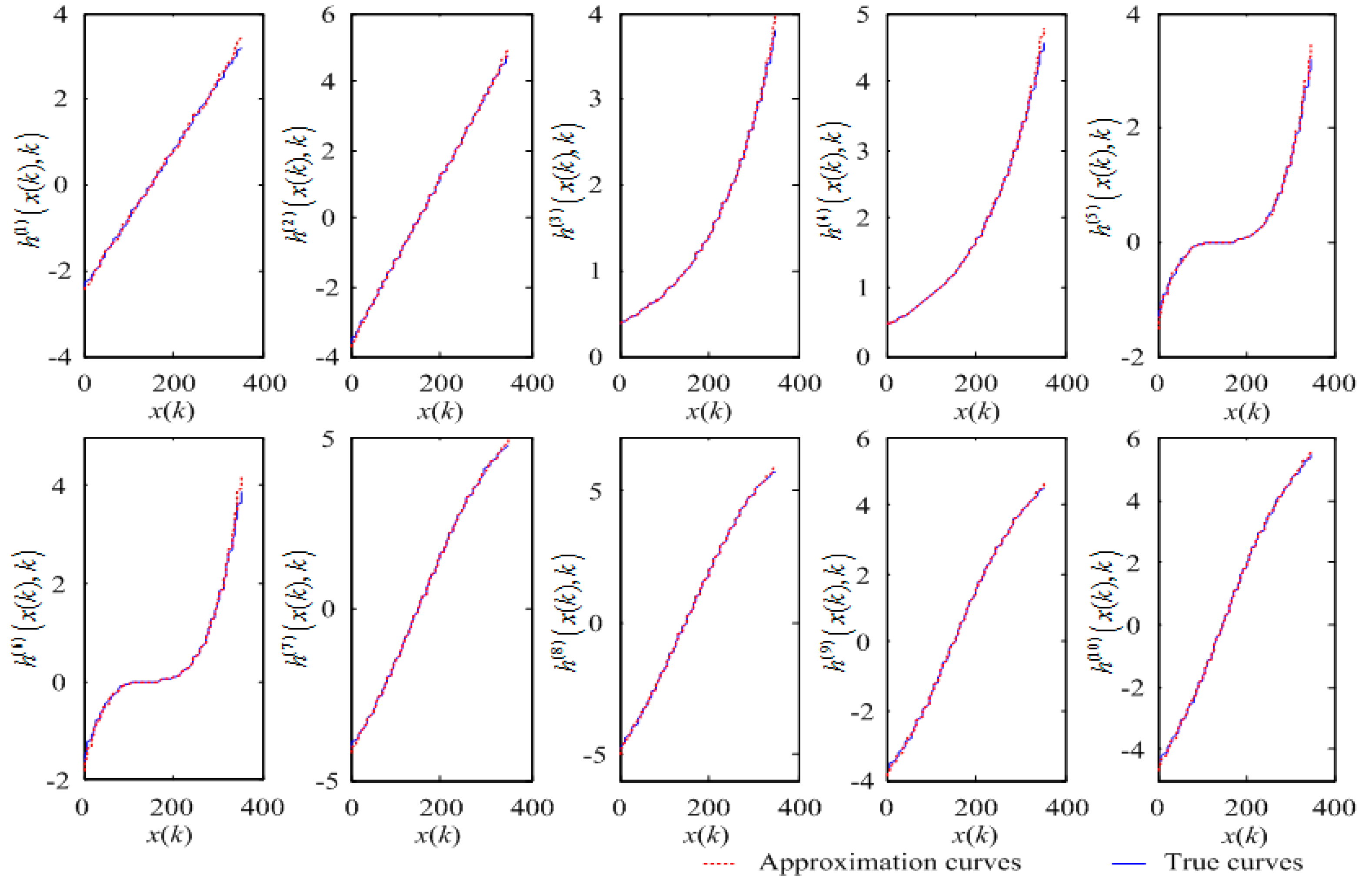
Because the state ranges from –3 to 4, we chose sampling points () to approximate, and the corresponding coefficients were , , and . Their mean square errors (MSEs) are shown in Table 1, and the approximation curves are shown in Figure 2.
To compare with other approximate methods, we introduced the approximation method using a McLaughlin series. We used a third-order McLaughlin series to approximate the nonlinear functions . The MSEs of the approximation algorithm, using a McLaughlin series, are also shown in Table 1. From Table 1, we can see that the MSEs of the approximation algorithm using a McLaughlin series are larger than that when using Gauss–Hermite approximation.
6.3. Estimation Using WMF-PF
From the above experiments, we see that the approximation effect is good when using the above coefficients. Next, we established the measurement equation and fusion matrix of WMF. As the intermediary function is , from Equations (24) and (25), the coefficient matrices , and its full rank decomposition matrices and , can be computed as follows:
Using the WMF-PF algorithm, we obtained the state estimate for the system in Equations (39) and (40). The curves of the true values and their estimates, using WMF-PF based on Gauss–Hermite approximation, are shown in Figure 3. The tracking performance is optimal.
6.4. Analysis
In order to compare our findings with other fusion algorithms, we introduced a kind of distributed fusion method, called a fast covariance intersection (CI) fusion algorithm [39]. Its calculation process is
where is the fusion estimate by CI, are the estimates of subsystems, are the filter error variance matrices of subsystems, and
Using the CI fusion algorithm and the PF algorithm, we obtained the covariance intersection PF (CI-PF). This fusion algorithm is simple, robust, and flexible. However, its accuracy is lower than WMF. We introduced an evaluation indicator called the accumulated mean square error (AMSE) [29]:
where is the jth-time Monte Carlo experiment at time t. The AMSE curves of local PFs (LF1–LF7), the WMF-PF, and the CI-PF are shown in Figure 4 with 20 Monte Carlo experiments. From Figure 4, the WMF-PF based on Gauss–Hermite approximation is shown to have better accuracy than local PF and CI-PF.
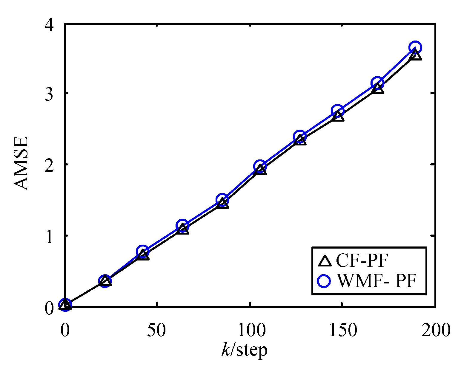
In addition, we simulated the AMSE curves of WMF-PF under ,, , , and and WMF-PF under , , , and . To distinguish them with the above WMF-PF, we named them WMF-PF-1 and WMF-PF-2. The AMSE curves of WMF-PF, WMF-PF-1, and WMF-PF-2 are shown in Figure 5. We can see that, as the interval becomes larger, the computational cost is reduced, but the estimation accuracy declines, and a reasonable parameter can improve the estimation accuracy. The AMSE curves of WMF-PF and CF-PF are shown in Figure 6. We can see that the accuracy of WMF-PF approximates that of CF-PF.
Next, we compare the computational cost of WMP-PF and CF-PF. Because is a matrix, the time complexity of WMP-PF is . However, is a matrix and its time complexity is . Therefore, the computational cost of WMF-PF is obviously lower than that of CF-PF.
In summary, the proposed WMP-PF, based on Gauss–Hermite approximation, is more accurate compared with local PFs, and has a lower computation cost when compared with CF-PF.
7. Conclusions
A general WMF algorithm is presented here for nonlinear multisensory systems based on the Gauss–Hermite approximation of nonlinear functions and the weighted least square method. An augmented high-dimension measurement from all sensors is compressed to a low-dimension one. Combined with the particle filter, the nonlinear weighted measurement fusion PF (WMF-PF) is presented. It can handle the nonlinear fusion estimation problem, and has reasonable accuracy and a reduced computational cost compared to centralized fusion PF. The proposed WMF algorithm can be used in systems of large-scale sensors, which can significantly reduce the computational cost and improve the real-time feature.
Acknowledgments
This work was supported by the Natural Science Foundation of China (No. 61573132 and No. 61503127), by the Natural Science Foundation of Heilongjiang province (No. F2015014), by Chang Jiang Scholar Candidates Program for Provincial Universities in Heilongjiang (No. 2013CJHB005), by the Science and Technology Innovative Research Team in Higher Educational Institutions of Heilongjiang Province (No. 2012TD007), and by the Electronic Engineering Province Key Laboratory.
Author Contributions
Shuli Sun proposed the algorithm. Yun Li derived the algorithm and wrote the paper. Gang Hao performed the simulation work.
Conflicts of Interest
The authors declare no conflict of interest.
References
- Gispan, L.; Leshem, A.; Be’ery, Y. Decentralized estimation of regression coefficients in sensor networks. Digit. Signal Proc. 2017, 68, 16–23. [Google Scholar] [CrossRef]
- Song, E.B.; Zhu, Y.M.; Zhou, J. Sensors’ optimal dimensionality compression matrix in estimation fusion. Automatica 2005, 41, 2131–2139. [Google Scholar] [CrossRef]
- Sun, S.; Lin, H.; Ma, J.; Li, X. Multi-sensor distributed fusion estimation with applications in networked systems: A review paper. Inf. Fusion 2017, 38, 122–134. [Google Scholar] [CrossRef]
- Sun, S.L.; Deng, Z.L. Multi-sensor optimal information fusion Kalman filter. Automatica 2004, 40, 1017–1023. [Google Scholar] [CrossRef]
- Ma, J.; Sun, S.L. Information fusion estimators for systems with multiple sensors of different packet dropout rates. Inf. Fusion 2011, 12, 213–222. [Google Scholar] [CrossRef]
- Tian, T.; Sun, S.L.; Li, N. Multi-sensor information fusion estimators for stochastic uncertain systems with correlated noises. Inf. Fusion 2016, 27, 126–137. [Google Scholar] [CrossRef]
- Ge, Q.B.; Shao, T.; Duan, Z.S.; Wen, C.L. Performance Analysis of the Kalman Filter with Mismatched Measurement Noise Covariance. IEEE Trans. Autom. Control 2016, 61, 4014–4019. [Google Scholar] [CrossRef]
- Carlson, N. Federated square root filter for decentralized parallel processes. IEEE Trans. Aerosp. Electron. Syst. 1990, 26, 517–525. [Google Scholar] [CrossRef]
- Kim, K. Development of track to track fusion algorithm. In Proceedings of the American Control Conference, Baltimore, MD, USA, 29 June–1 July 1994. [Google Scholar]
- Julier, S.; Uhlmann, J. A non-divergent estimation algorithm in the presence of unknown correlation. In Proceedings of the American Control Conference, Albuquerque, NM, USA, 6 June 1997; pp. 2369–2373. [Google Scholar]
- Qiang, G.; Harris, C.J. Comparison of two measurement fusion methods for Kalman-filter-based multisensor data fusion. IEEE Trans. Aerosp. Electron. Syst. 2001, 37, 273–280. [Google Scholar] [CrossRef]
- Oussalah, M.; Messaoudi, Z.; Ouldali, A. Track-to-Track Measurement Fusion Architectures and Correlation Analysis. J. Univers. Comput. Sci. 2010, 16, 37–61. [Google Scholar]
- Ran, C.J.; Deng, Z.L. Self-tuning weighted measurement fusion Kalman filtering algorithm. Comput. Stat. Data Anal. 2012, 56, 2112–2128. [Google Scholar] [CrossRef]
- Li, X.R.; Jilkov, V.P. A Survey of Maneuvering Target Tracking: Approximation Techniques for Nonlinear Filtering. Proc. SPIE 2004, 5428, 537–550. [Google Scholar] [CrossRef]
- Bar-Shalom, Y.; Li, X.R. Multitarget-Multisensor Tracking: Principles and Techniques; YBS Publishing: Storrs, CT, USA, 1995. [Google Scholar]
- Assa, A.; Janabi-Sharifi, F. A Kalman Filter-Based Framework for Enhanced Sensor Fusion. IEEE Sens. J. 2015, 15, 3281–3292. [Google Scholar] [CrossRef]
- Straka, O.; Duník, J.; Šimandl, M. Truncation nonlinear filters for state estimation with nonlinear inequality constraints. Automatica 2012, 48, 273–286. [Google Scholar] [CrossRef]
- Hlinka, O.; Slučiak, O.; Hlawatsch, F.; Djuric, P.M.; Rupp, M. Likelihood consensus and its application to distributed particle filtering. IEEE Trans. Signal Proc. 2012, 60, 4334–4349. [Google Scholar] [CrossRef]
- Ge, Q.B.; Xu, D.X.; Wen, C.L. Cubature information filters with correlated noises and their applications in decentralized fusion. Signal Proc. 2014, 94, 434–444. [Google Scholar] [CrossRef]
- Jia, B.; Xin, M.; Cheng, Y. High-degree cubature Kalman filter. Automatica 2013, 49, 510–518. [Google Scholar] [CrossRef]
- Khaleghi, B.; Khamis, A.; Karray, F.O.; Razavi, S.N. Multisensor data fusion: A review of the state-of-the-art. Inf. Fusion 2013, 14, 28–44. [Google Scholar] [CrossRef]
- Julier, S.J.; Uhlmann, J.K. A new extension of the Kalman filter to nonlinear systems. In Proceedings of the International Symposium on Aerospace/Defense Sensing, Simulation and Controls, Orlando, FL, USA, 28 July 1997. [Google Scholar]
- Julier, S.J.; Uhlmann, J.K. Unscented filtering and nonlinear estimation. Proc. IEEE 2004, 92, 401–422. [Google Scholar] [CrossRef]
- Arulampalam, S.; Maskell, S.; Gordon, N.; Clapp, T. A tutorial on particle filters for online nonlinear/non-Gaussian Bayesian tracking. IEEE Trans. Signal Proc. 2002, 50, 174–188. [Google Scholar] [CrossRef]
- Chatzi, E.N.; Smyth, A.W. The unscented Kalman filter and particle filter methods for nonlinear structural system identification with non-collocated heterogeneous sensing. Struct. Control Health Monit. 2009, 16, 99–123. [Google Scholar] [CrossRef]
- Azam, E.S. Online damage detection in structural systems: Applications of proper orthogonal decomposition, and Kalman and particle filters. Springerbriefs Appl. Sci. Technol. 2014, 1–45. [Google Scholar] [CrossRef]
- Mirzazadeh, R.; Azam, E.S.; Mariani, S. Micromechanical characterization of polysilicon films through on-chip tests. Sensors 2016, 16. [Google Scholar] [CrossRef] [PubMed]
- Cacace, F.; Germanib, A.; Palumboc, P. The observer follower filter: A new approach to nonlinear suboptimal filtering. Automatica 2013, 49, 548–553. [Google Scholar] [CrossRef]
- Hao, G.; Sun, S.L.; Li, Y. Nonlinear weighted measurement fusion Unscented Kalman Filter with asymptotic optimality. Inf. Sci. 2015, 299, 85–98. [Google Scholar] [CrossRef]
- Pomorski, K. Gauss-Hermite approximation formula. Comput. Phys. Commun. 2006, 174, 181–186. [Google Scholar] [CrossRef]
- Santhanam, B.; Santhanam, T.S. On discrete Gauss-Hermite functions and eigenvectors of the discrete Fourier transform. Signal Proc. 2008, 88, 2738–2746. [Google Scholar] [CrossRef]
- Strutinsky, V.M. Shells in deformed nuclei. Nucl. Phys. A 1968, 122, 1–33. [Google Scholar] [CrossRef]
- Strutinsky, V.M. Shell effects in nuclear masses and deformation energies. Nucl. Phys. A 1967, 95, 420–442. [Google Scholar] [CrossRef]
- Ge, Q.; Shao, T.; Chen, S.D.; Wen, C.L. Carrier Tracking Estimation Analysis by Using the Extended Strong Tracking Filtering. IEEE Trans. Ind. Electron. 2017, 64, 1415–1424. [Google Scholar] [CrossRef]
- Moradkhani, H.; Hsu, K.L.; Gupta, H.; Sorooshian, S. Uncertainty assessment of hydrologic model states and parameters: Sequential data assimilation using the particle filter. Water Resour. Res. 2005, 41, 237–246. [Google Scholar] [CrossRef]
- Yuen, K.V.; Hoi, K.I.; Mok, K.M. Selection of noise parameters for Kalman filter. Earthq. Eng. Eng. Vib. 2007, 6, 49–56. [Google Scholar] [CrossRef]
- Kontoroupi, T.; Smyth, A.W. Online Noise Identification for Joint State and Parameter Estimation of Nonlinear Systems; ASCE: Reston, VA, USA, 2015. [Google Scholar]
- Kitagawa, G. Non-Gaussian state space modeling of time series. In Proceedings of the 26th Conference on Decision and Control, Los Angeles, CA, USA, 9–11 December 1987; pp. 1700–1705. [Google Scholar]
- Cong, J.; Li, Y.; Qi, G.; Sheng, A. An order insensitive sequential fast covariance intersection fusion algorithm. Inf. Sci. 2016, 367–368, 28–40. [Google Scholar] [CrossRef]
Figure 1.
Flow chart of the weighted measurement fusion particle filter (WMF-PF) algorithm.
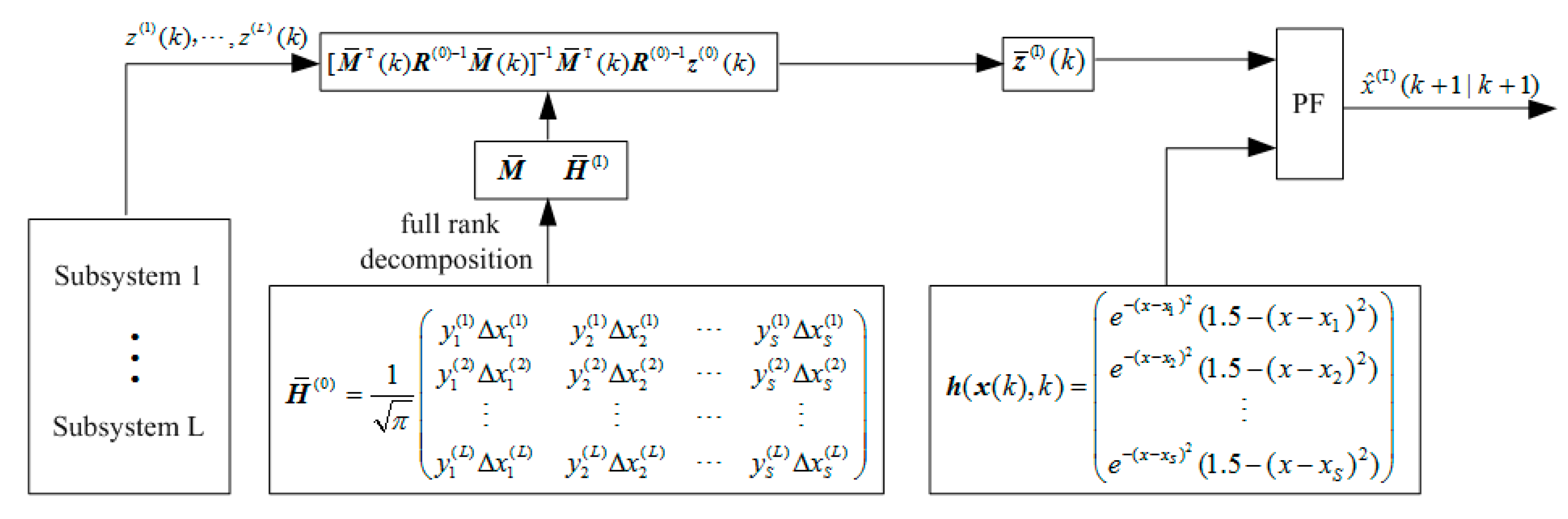
Figure 2.
Approximation curves of nonlinear functions.

Figure 3.
Curves of the true values and estimates using the WMF-PF algorithm based on Gauss–Hermite approximation.
Figure 3.
Curves of the true values and estimates using the WMF-PF algorithm based on Gauss–Hermite approximation.
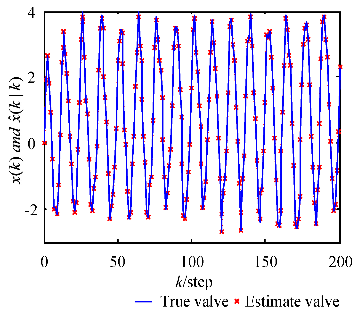
Figure 4.
Accumulated mean square error (AMSE) curves of local particle filters (PFs), WMF-PF, and covariance intersection PF (CI-PF).
Figure 4.
Accumulated mean square error (AMSE) curves of local particle filters (PFs), WMF-PF, and covariance intersection PF (CI-PF).
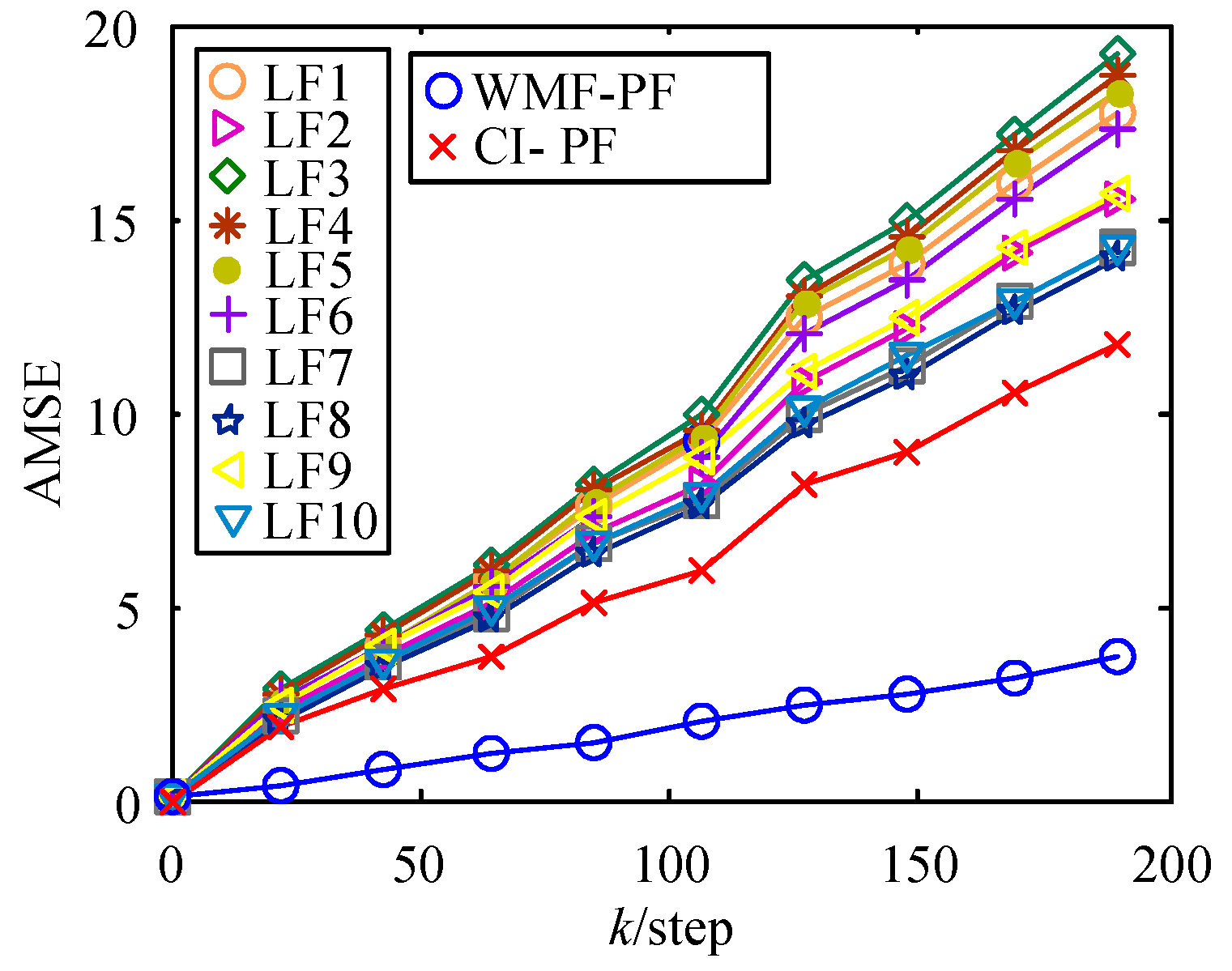
Figure 5.
AMSE curves of WMF-PF, WMF-PF-1, and WMF-PF-2.

Figure 6.
AMSE curves of WMF-PF and CF-PF.

Table 1.
Mean square errors.
| Sensor Functions | ||||||||||
| MSEs using Gauss–Hermite | 0.0032 | 0.0017 | 0.0010 | 0.0014 | 0.0029 | 0.0042 | 0.0009 | 0.0013 | 0.0010 | 0.0015 |
| MSEs using McLaughlin series | 0 | 0 | 0.0258 | 0.0371 | 0.9621 | 1.3854 | 0.2286 | 0.3292 | 0.3963 | 0.5707 |
© 2017 by the authors. Licensee MDPI, Basel, Switzerland. This article is an open access article distributed under the terms and conditions of the Creative Commons Attribution (CC BY) license (http://creativecommons.org/licenses/by/4.0/).
Share and Cite
MDPI and ACS Style
Li, Y.; Sun, S.L.; Hao, G. A Weighted Measurement Fusion Particle Filter for Nonlinear Multisensory Systems Based on Gauss–Hermite Approximation. Sensors 2017, 17, 2222. https://doi.org/10.3390/s17102222
AMA Style
Li Y, Sun SL, Hao G. A Weighted Measurement Fusion Particle Filter for Nonlinear Multisensory Systems Based on Gauss–Hermite Approximation. Sensors. 2017; 17(10):2222. https://doi.org/10.3390/s17102222
Chicago/Turabian StyleLi, Yun, Shu Li Sun, and Gang Hao. 2017. "A Weighted Measurement Fusion Particle Filter for Nonlinear Multisensory Systems Based on Gauss–Hermite Approximation" Sensors 17, no. 10: 2222. https://doi.org/10.3390/s17102222
Note that from the first issue of 2016, this journal uses article numbers instead of page numbers. See further details here.