Low Computational-Cost Footprint Deformities Diagnosis Sensor through Angles, Dimensions Analysis and Image Processing Techniques

 , , and
Abstract
:1. Introduction
2. Materials and Methods
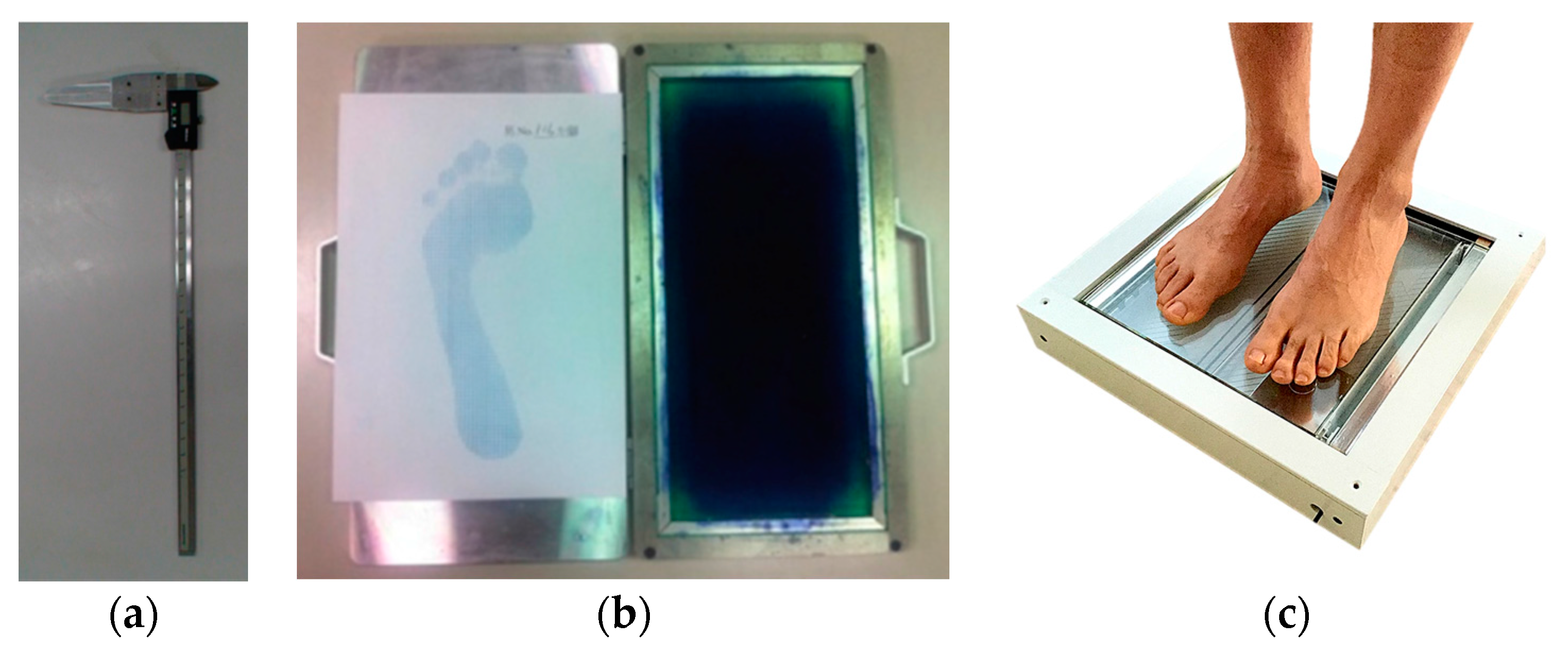
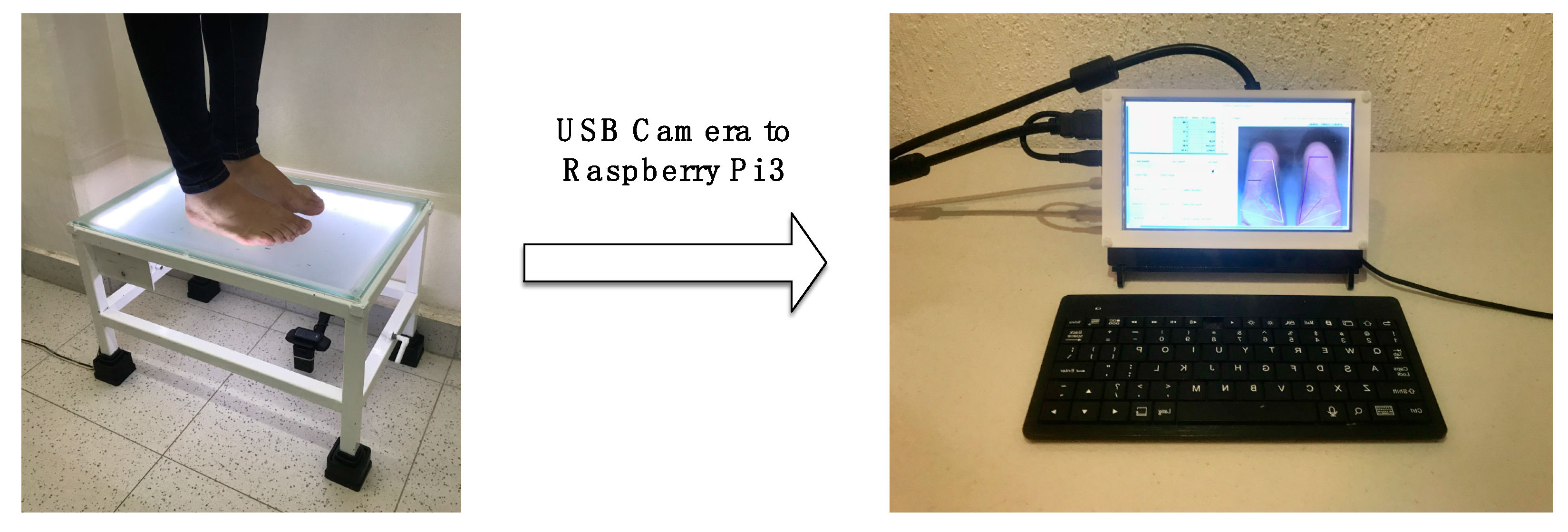
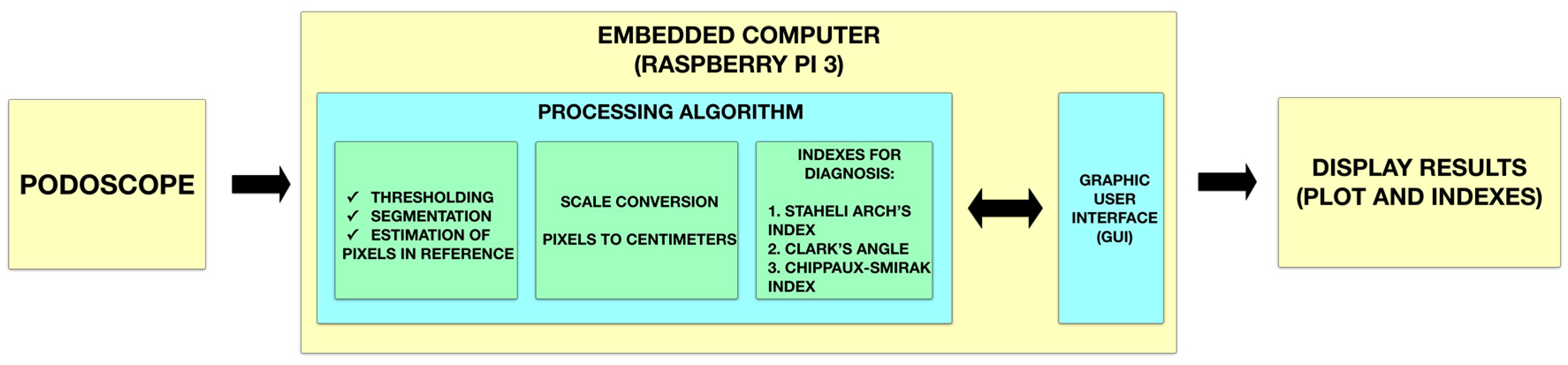
2.1. Smart Sensor Setup
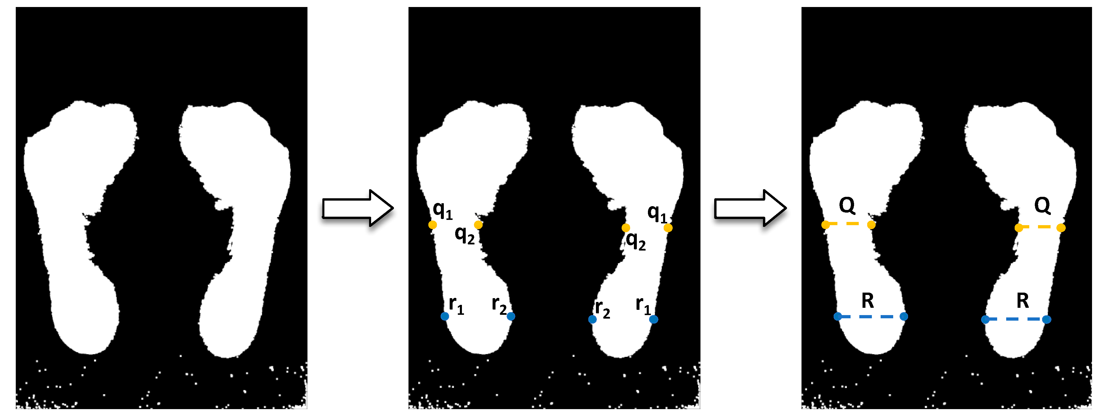
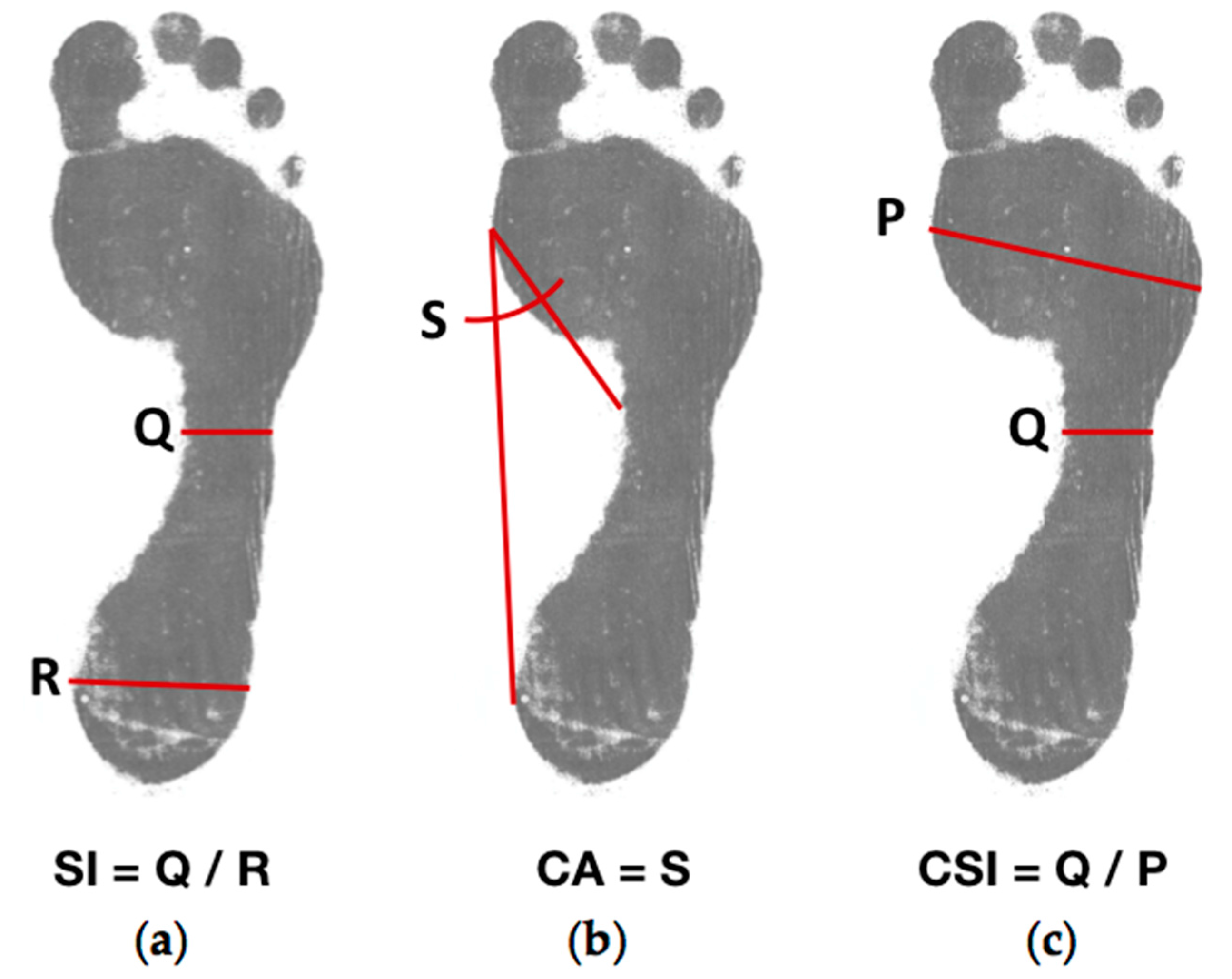
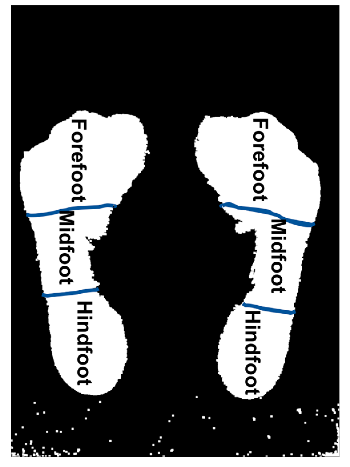
2.2. Footprint Parameters
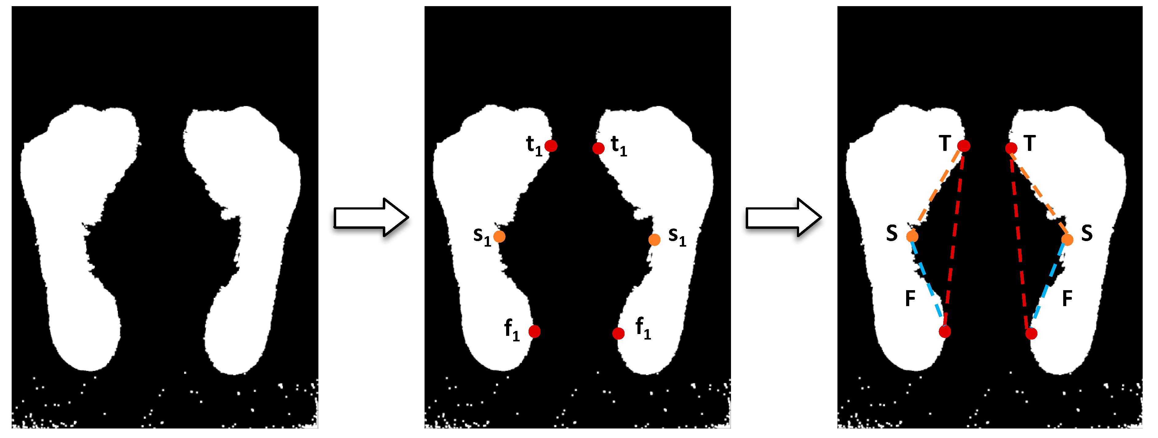
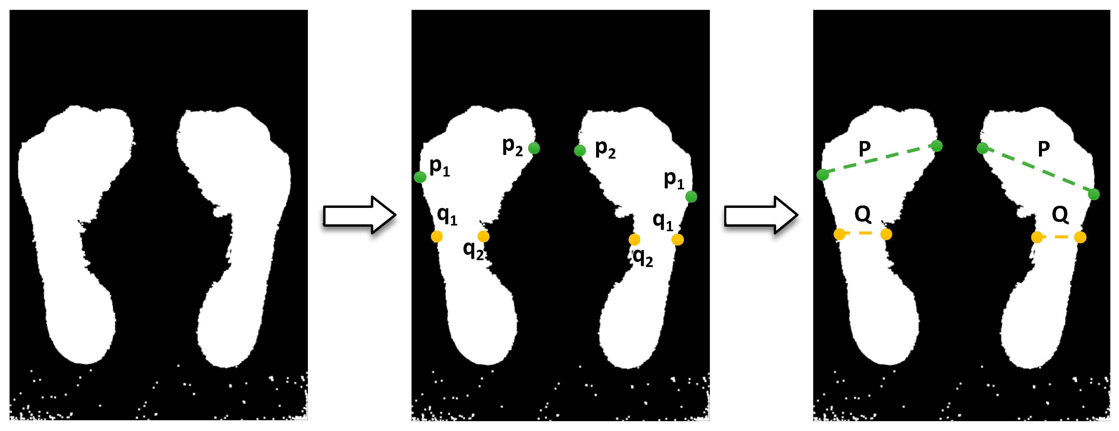
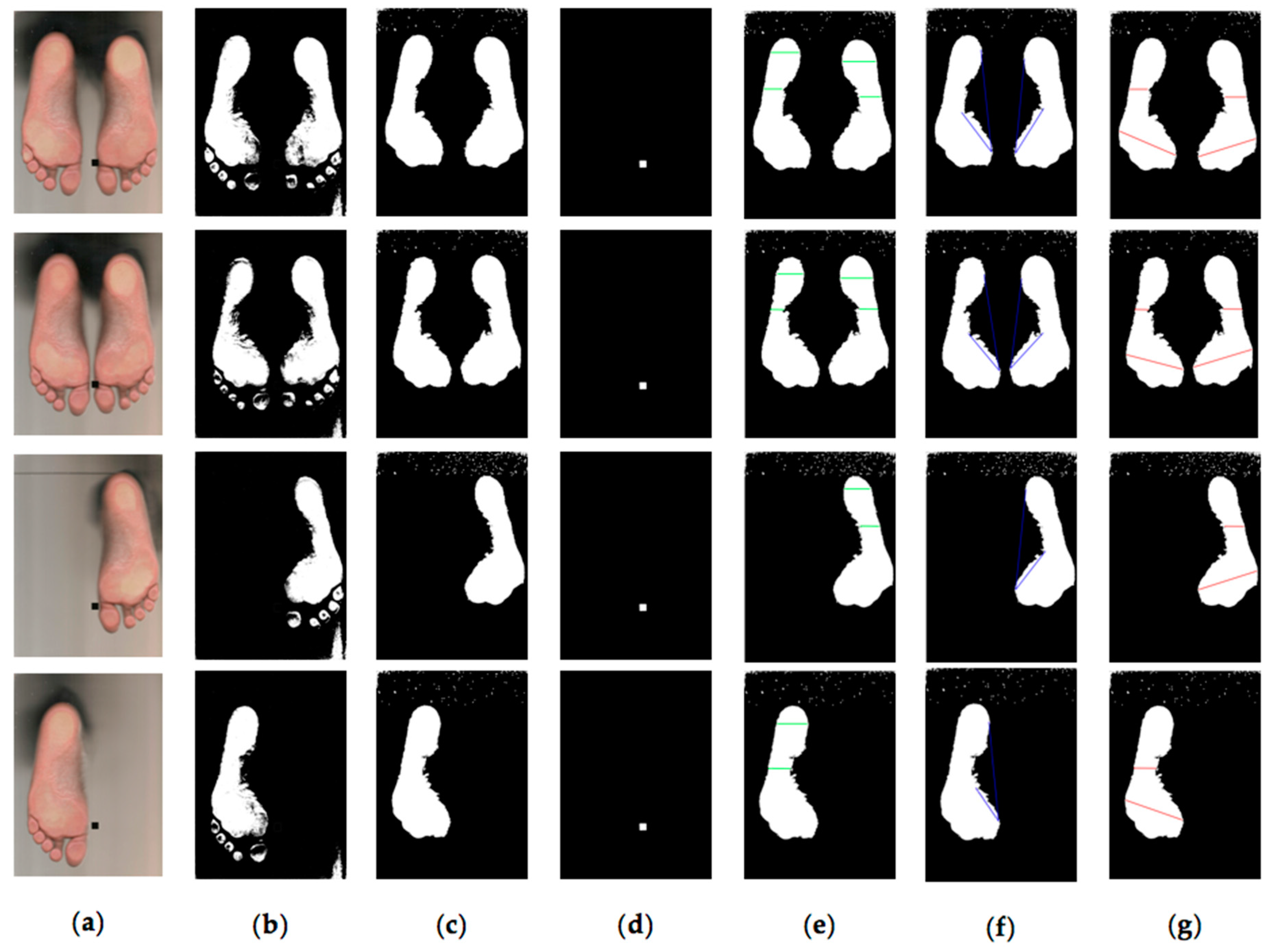
2.3. Algorithms for Estimation of Measures in Footprint
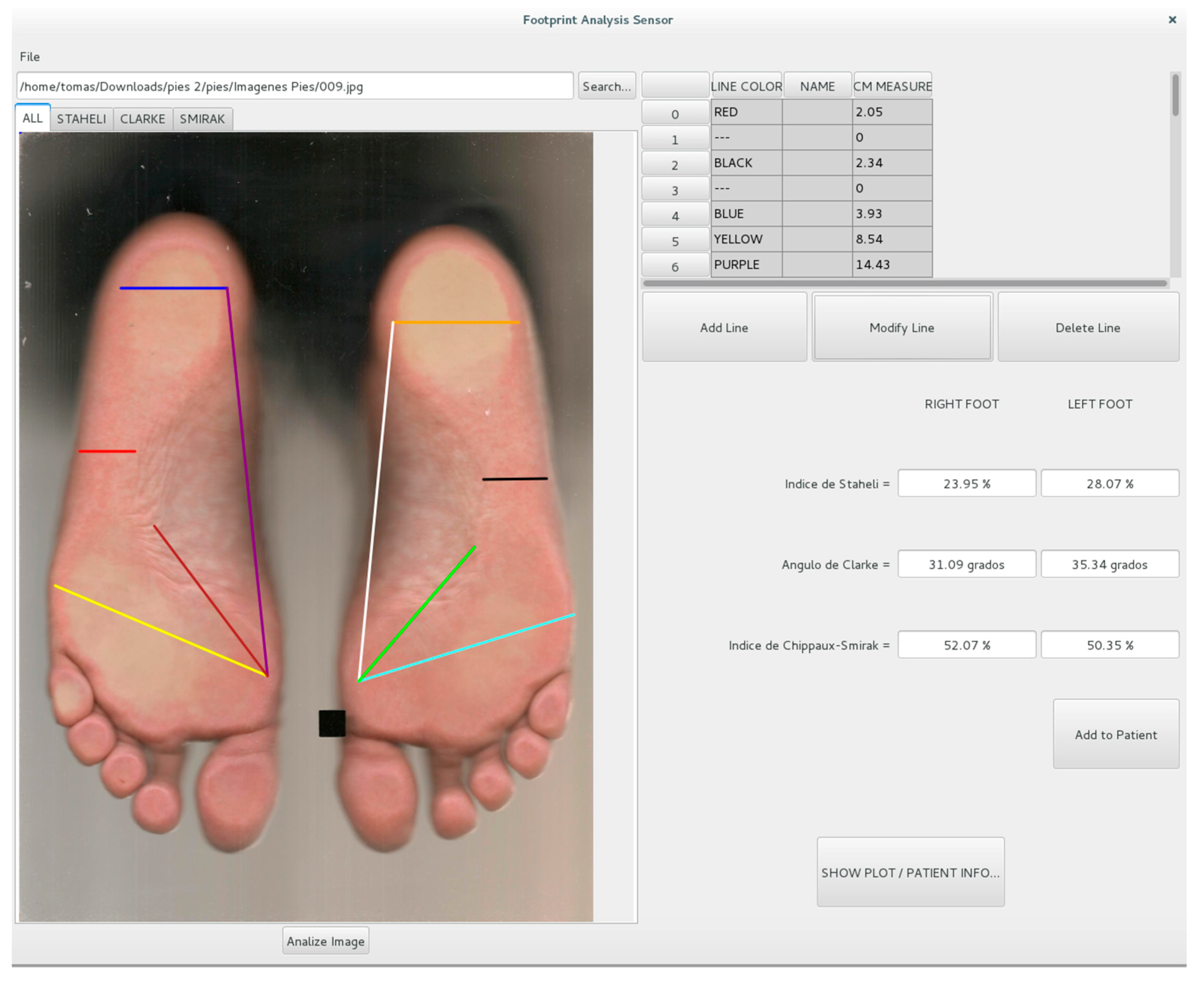
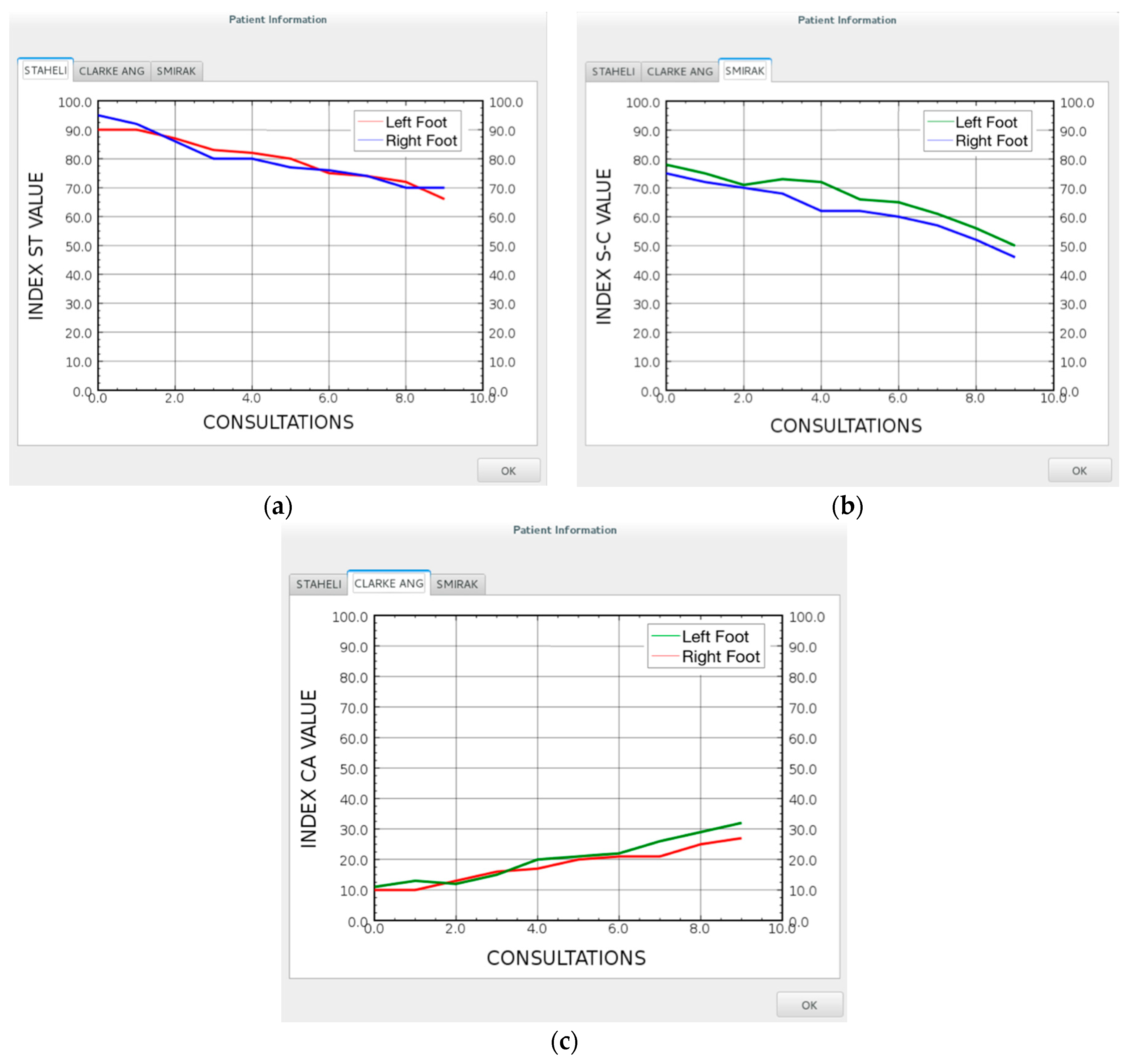
2.4. Graphic User Interface
2.5. Experimental Setup
3. Results
4. Discussion and Conclusions
Acknowledgments
Author Contributions
Conflicts of Interest
Ethical Statements
References
- Queen, R.M.; Mall, N.A.; Hardaker, W.M.; Nunley, J.A. Describing the medial longitudinal arch using footprint indices and a clinical grading system. Foot Ankle Int. 2007, 28, 456–462. [Google Scholar] [PubMed]
- Kouchi, M.; Mochimaru, M.; Tsuzuki, K.; Yokoi, T. Interobserver errors in anthropometry. J. Hum. Ergol. 1999, 28, 15–24. [Google Scholar]
- Lee, Y.-C.; Lin, G.; Wang, M.-J.J. Comparing 3D foot scanning with conventional measurement methods. J. Foot Ankle Res. 2014, 7, 44. [Google Scholar] [CrossRef] [PubMed]
- Mall, N.A.; Hardaker, W.M.; Nunley, J.A.; Queen, R.M. The reliability and reproducibility of foot type measurements using a mirrored foot photo box and digital photography compared to caliper measurements. J. Biomech. 2007, 40, 1171–1176. [Google Scholar] [CrossRef] [PubMed]
- Van Boerum, D.H.; Sangeorzan, B.J. Biomechanics and pathophysiology of flat foot. Foot Ankle Clin. 2003, 8, 419–430. [Google Scholar] [CrossRef]
- Navarro, L.A.; García, D.O.; Villavicencio, E.A.; Torres, M.A.; Nakamura, O.K.; Huamaní, R.; Yabar, L.F. Opto-electronic system for detection of flat foot by using estimation techniques: Study and approach of design. In Proceedings of the 2010 Annual International Conference of the IEEE Engineering in Medicine and Biology Society (EMBC), Buenos Aires, Argentina, 31 August–4 September 2010; pp. 5768–5771. [Google Scholar]
- Hamza, A.O.; Ahmed, H.K.; Khider, M.O. A new noninvasive flatfoot detector. J. Clin. Eng. 2015, 40, 57–63. [Google Scholar] [CrossRef]
- Guerrero-Turrubiates, J.D.J.; Cruz-Aceves, I.; Ledesma, S.; Sierra-Hernandez, J.M.; Velasco, J.; Avina-Cervantes, J.G.; Avila-Garcia, M.S.; Rostro-Gonzalez, H.; Rojas-Laguna, R. Fast parabola detection using estimation of distribution algorithms. Comput. Math. Methods Med. 2017, 2017, 6494390. [Google Scholar] [CrossRef] [PubMed]
- Bates, K.; Savage, R.; Pataky, T.; Morse, S.; Webster, E.; Falkingham, P.; Ren, L.; Qian, Z.; Collins, D.; Bennett, M. Does footprint depth correlate with foot motion and pressure? J. R. Soc. Interface 2013, 10, 20130009. [Google Scholar] [PubMed]
- Cheung, J.T.-M.; Zhang, M. A 3-dimensional finite element model of the human foot and ankle for insole design. Arch. Phys. Med. Rehabil. 2005, 86, 353–358. [Google Scholar] [CrossRef] [PubMed]
- Morales-Orcajo, E.; Bayod, J.; de Las Casas, E.B. Computational foot modeling: Scope and applications. Arch. Comput. Methods Eng. 2016, 23, 389–416. [Google Scholar]
- Chun, S.; Kong, S.; Mun, K.-R.; Kim, J. A foot-arch parameter measurement system using a RGB-D camera. Sensors 2017, 17, 1796. [Google Scholar] [CrossRef] [PubMed]
- Burns, J.; Keenan, A.-M.; Redmond, A. Foot type and overuse injury in triathletes. J. Am. Podiatr. Med. Assoc. 2005, 95, 235–241. [Google Scholar] [CrossRef] [PubMed]
- Chuckpaiwong, B.; Nunley, J.A.; Mall, N.A.; Queen, R.M. The effect of foot type on in-shoe plantar pressure during walking and running. Gait Posture 2008, 28, 405–411. [Google Scholar] [CrossRef] [PubMed]
- Dahle, L.K.; Mueller, M.; Delitto, A.; Diamond, J.E. Visual assessment of foot type and relationship of foot type to lower extremity injury. J. Orthop. Sports Phys. Ther. 1991, 14, 70–74. [Google Scholar] [CrossRef] [PubMed]
- Staheli, L.T.; Chew, D.E.; Corbett, M. The longitudinal arch. J. Bone Joint Surg. Am. 1987, 69, 426–428. [Google Scholar] [PubMed]
- Plumarom, Y.; Imjaijitt, W.; Chaiphrom, N. Comparison between staheli index on harris mat footprint and talar-first metatarsal angle for the diagnosis of flatfeet. J. Med. Assoc. Thail. 2014, 97, S131–S135. [Google Scholar]
- Shiang, T.-Y.; Lee, S.-H.; Lee, S.-J.; Chu, W.C. Evaluating different footprints parameters as a predictor of arch height. IEEE Eng. Med. Biol. Mag. 1998, 17, 62–66. [Google Scholar] [CrossRef] [PubMed]
- Bradski, G. Opencv library. Dr. Dobbs’s J. 2000, 25, 120–126. [Google Scholar]
- Vazquez-Cruz, M.; Jimenez-Garcia, S.; Luna-Rubio, R.; Contreras-Medina, L.; Vazquez-Barrios, E.; Mercado-Silva, E.; Torres-Pacheco, I.; Guevara-Gonzalez, R. Application of neural networks to estimate carotenoid content during ripening in tomato fruits (solanum lycopersicum). Sci. Hortic. 2013, 162, 165–171. [Google Scholar] [CrossRef]
- Aruntammanak, W.; Aunhathaweesup, Y.; Wongseree, W.; Leelasantitham, A.; Kiattisin, S. Diagnose flat foot from foot print image based on neural network. In Proceedings of the 2013 6th Biomedical Engineering International Conference (BMEiCON), Amphur Muang, Thailand, 23–25 October 2013; pp. 1–5. [Google Scholar]
- Cavanagh, P.R.; Rodgers, M.M. The arch index: A useful measure from footprints. J. Biomech. 1987, 20, 547–551. [Google Scholar] [CrossRef]
- Fernandez-Jaramillo, A.A.; de Jesus Romero-Troncoso, R.; Duarte-Galvan, C.; Torres-Pacheco, I.; Guevara-Gonzalez, R.G.; Contreras-Medina, L.M.; Herrera-Ruiz, G.; Millan-Almaraz, J.R. FPGA-based chlorophyll fluorescence measurement system with arbitrary light stimulation waveform using direct digital synthesis. Measurement 2015, 75, 12–22. [Google Scholar] [CrossRef]
- Ghasemi, A.; Zahediasl, S. Normality tests for statistical analysis: A guide for non-statisticians. Int. J. Endocrinol. Metab. 2012, 10, 486–489. [Google Scholar] [CrossRef] [PubMed]
- De La Fuente, J.L.M. General Podology and Biomechanics; Elsevier: Barcelona, Spain, 2009. [Google Scholar]
- Drapé, J.-L. Diagnostic Imaging of Foot Conditions; Elsevier: Barcelona, Spain, 2000. [Google Scholar]
- Núñez-Samper, M.; Alcázar, L.F.L. Biomechanics, Medicine and Surgery of the Foot; Elsevier: Barcelona, Spain, 2007. [Google Scholar]
- Lawrence, I.; Lin, K. A concordance correlation coefficient to evaluate reproducibility. Biometrics 1989, 45, 255–268. [Google Scholar]
- Fascione, J.M.; Crews, R.T.; Wrobel, J.S. Dynamic footprint measurement collection technique and intrarater reliability: Ink mat, paper pedography, and electronic pedography. J. Am. Podiatr. Med. Assoc. 2012, 102, 130–138. [Google Scholar] [CrossRef] [PubMed]
- Su, K.-H.; Kaewwichit, T.; Tseng, C.-H.; Chang, C.-C. Automatic footprint detection approach for the calculation of arch index and plantar pressure in a flat rubber pad. Multimed. Tools Appl. 2016, 75, 9757–9774. [Google Scholar] [CrossRef]


| Authors/Method | Objective of the Method | Type of Sensor | Accuracy |
|---|---|---|---|
| Navarro et al. [6] | Detection of flat foot using estimation techniques | Pressure sensors | N/A 1 |
| Hamza et al. [7] | Flatfoot detector using the height of the arch | Ultrasonic sensors | 100% in 20 subjects |
| Guerrero-Turrubiates et al. [8] | Detection of parabolas dimensions in the footprint | Footprint scanner | N/A 1 |
| Chun et al. [12] | 3D image reconstruction of the footprint | RGB-D camera | ~97.32% in 11 subjects 2 |
| FPDSS | Detection of deformities in the footprint through image processing | RGB camera with reference | 99.38% in 40 subjects 2 |
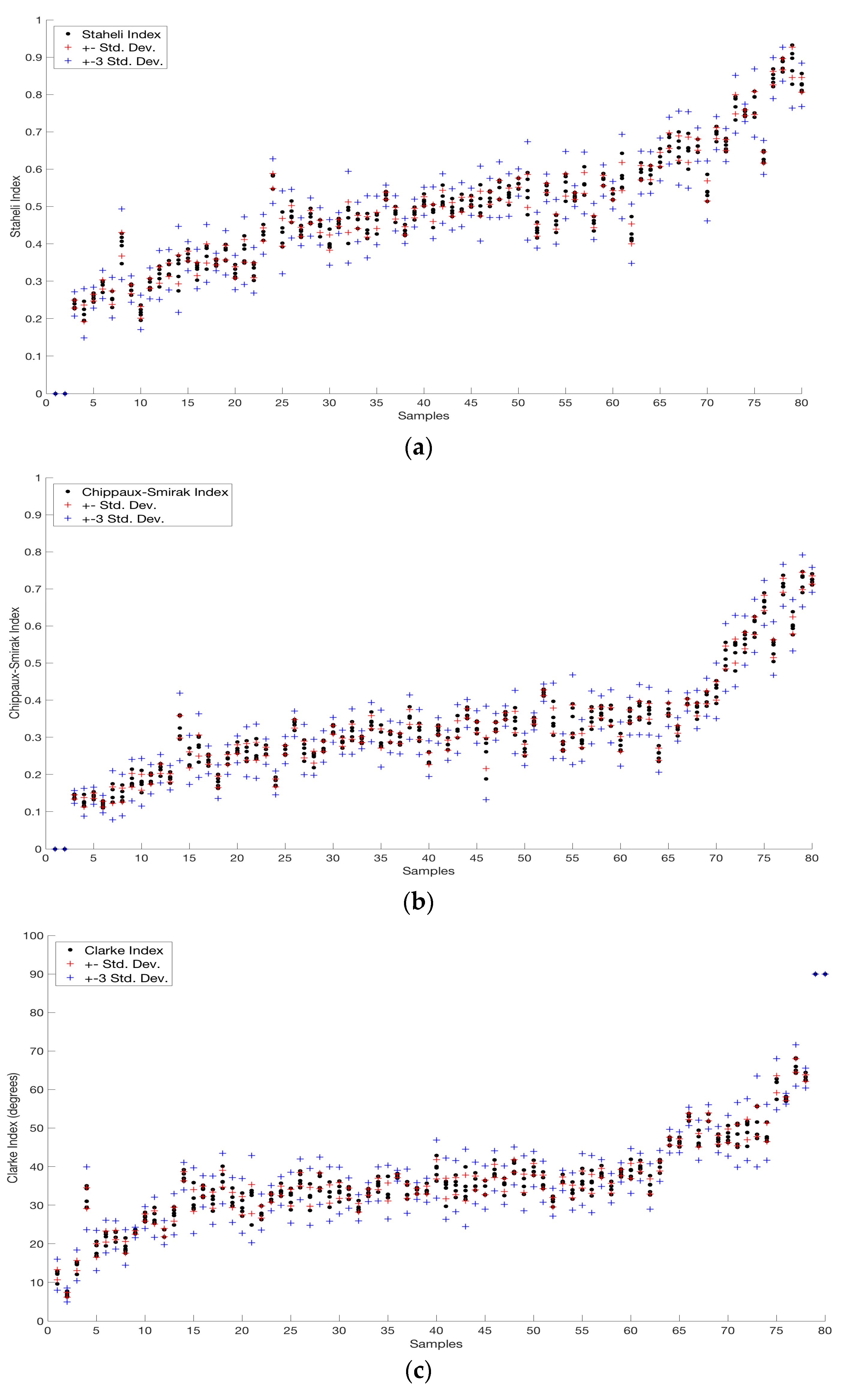
| Index Name | Amount of Values out of 1σ Rule | ||
|---|---|---|---|
| 2 | 1 | 0 | |
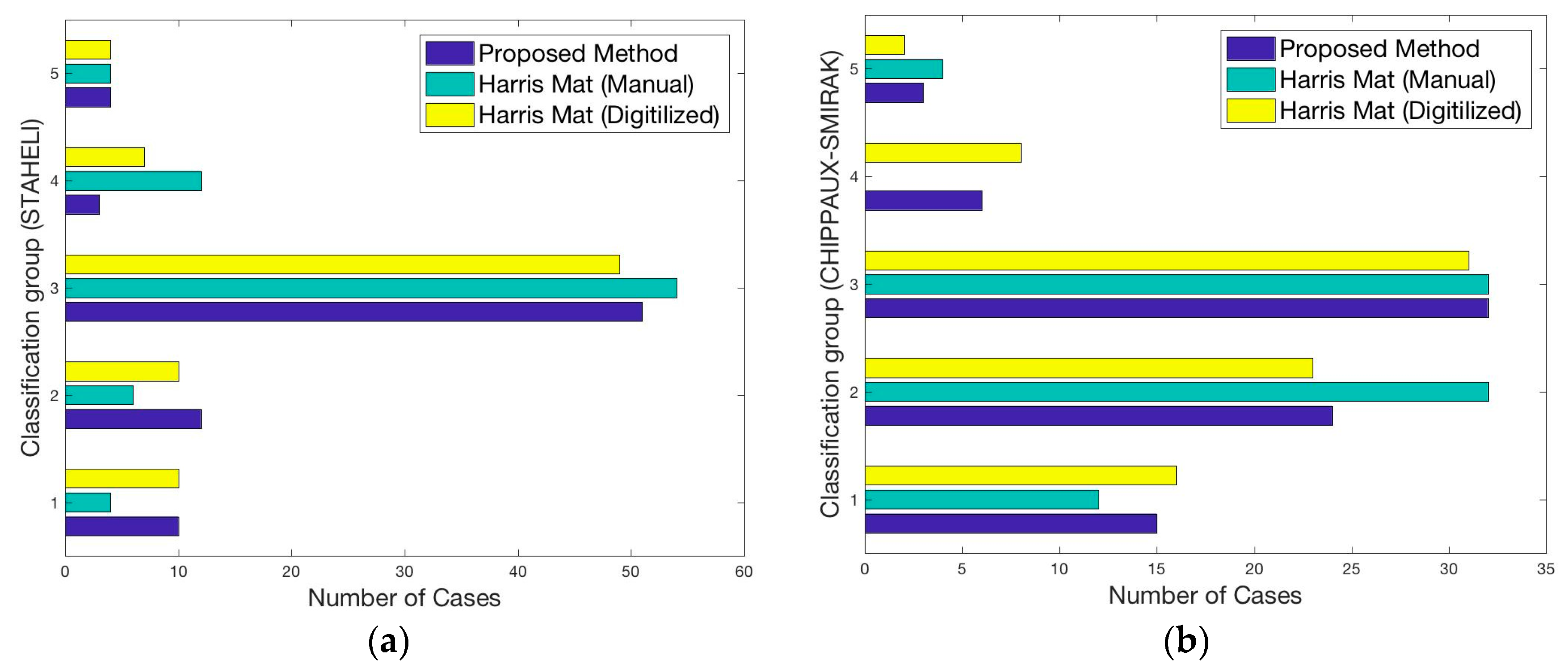
| Staheli Index | 14 | 57 | 9 |
| Chippaux-Smirak Index | 18 | 46 | 16 |
| Clarke Index | 12 | 49 | 19 |
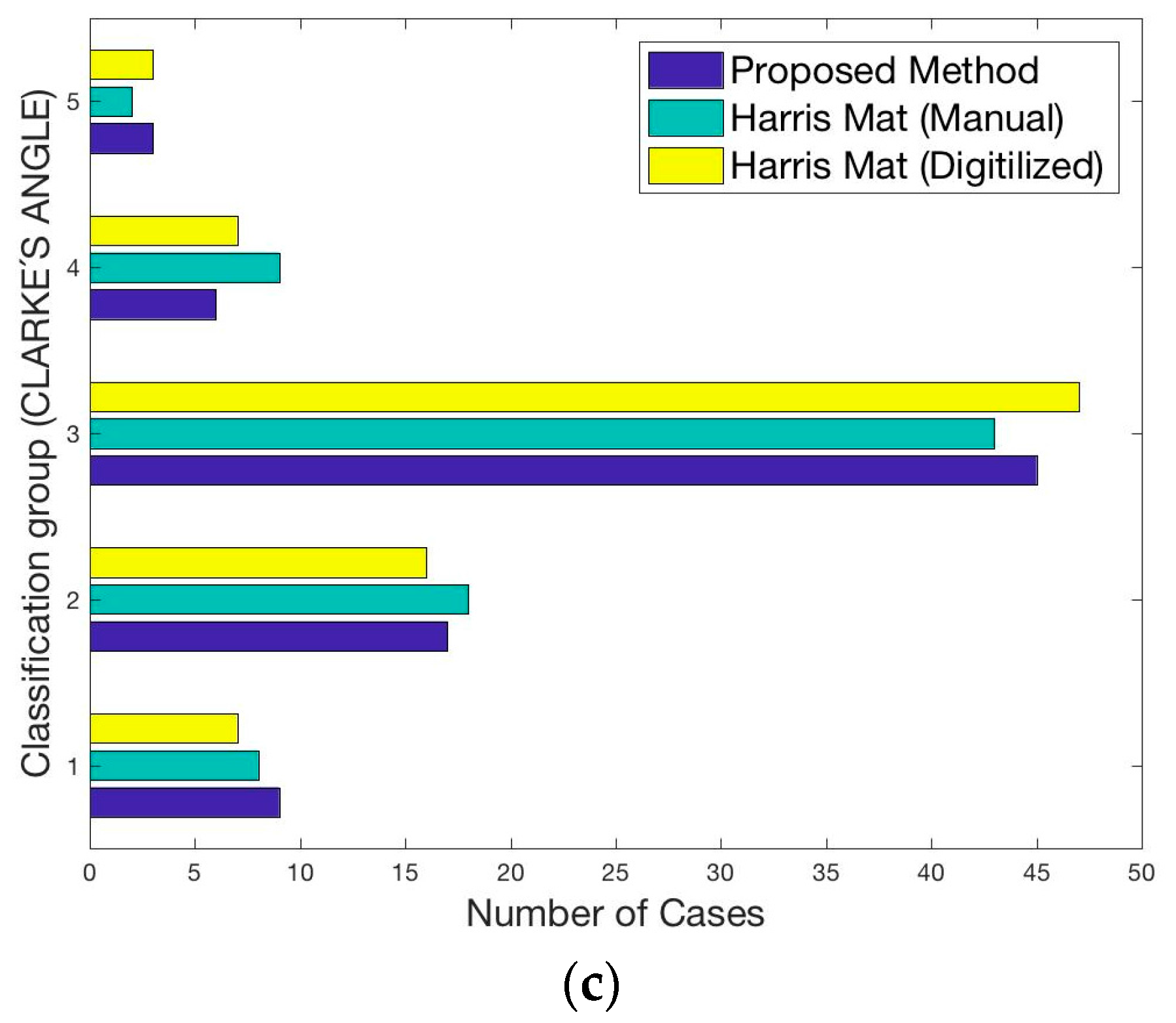
| Index Name | Classification Groups | ||||
|---|---|---|---|---|---|
| 1 | 2 | 3 | 4 | 5 | |
| Staheli Index | <0.3 | 0.3–0.4 | 0.4–0.7 | 0.7–0.8 | >0.8 |
| Chippaux-Smirak Index | <0.22 | 0.22–0.3 | 0.3–0.5 | 0.5–0.7 | >0.7 |
| Clarke Index | >50 | 38–50 | 26–38 | 15–26 | <15 |
| Compared Methods | Correlation Coefficient 1 |
|---|---|
| Ink mat (manual) vs. Ink mat (digitalized) | 0.9618 |
| FPDSS 2 vs. Ink mat (manual) | 0.9619 |
| FPDSS 2 vs. Ink mat (digitalized) | 0.9938 |
© 2017 by the authors. Licensee MDPI, Basel, Switzerland. This article is an open access article distributed under the terms and conditions of the Creative Commons Attribution (CC BY) license (http://creativecommons.org/licenses/by/4.0/).
Share and Cite
Maestre-Rendon, J.R.; Rivera-Roman, T.A.; Sierra-Hernandez, J.M.; Cruz-Aceves, I.; Contreras-Medina, L.M.; Duarte-Galvan, C.; Fernandez-Jaramillo, A.A. Low Computational-Cost Footprint Deformities Diagnosis Sensor through Angles, Dimensions Analysis and Image Processing Techniques. Sensors 2017, 17, 2700. https://doi.org/10.3390/s17112700
Maestre-Rendon JR, Rivera-Roman TA, Sierra-Hernandez JM, Cruz-Aceves I, Contreras-Medina LM, Duarte-Galvan C, Fernandez-Jaramillo AA. Low Computational-Cost Footprint Deformities Diagnosis Sensor through Angles, Dimensions Analysis and Image Processing Techniques. Sensors. 2017; 17(11):2700. https://doi.org/10.3390/s17112700
Chicago/Turabian StyleMaestre-Rendon, J. Rodolfo, Tomas A. Rivera-Roman, Juan M. Sierra-Hernandez, Ivan Cruz-Aceves, Luis M. Contreras-Medina, Carlos Duarte-Galvan, and Arturo A. Fernandez-Jaramillo. 2017. "Low Computational-Cost Footprint Deformities Diagnosis Sensor through Angles, Dimensions Analysis and Image Processing Techniques" Sensors 17, no. 11: 2700. https://doi.org/10.3390/s17112700