Out-of-Focus Projector Calibration Method with Distortion Correction on the Projection Plane in the Structured Light Three-Dimensional Measurement System

Abstract
:1. Introduction
2. Mathematical Model
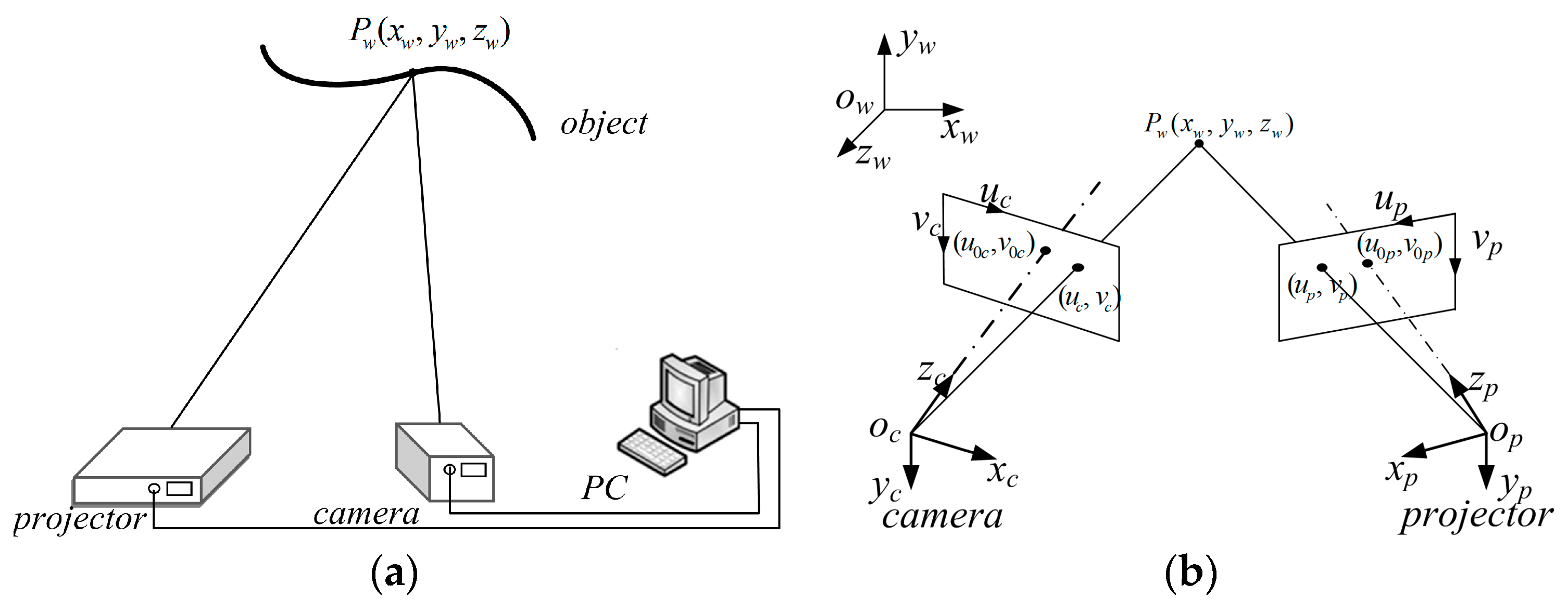
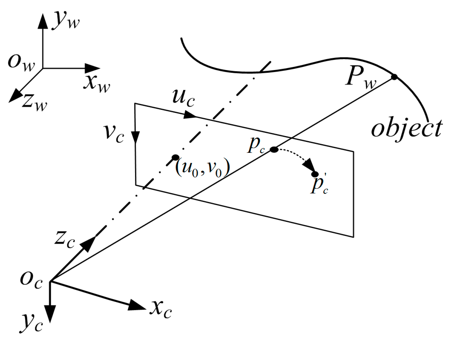
2.1. Camera Model
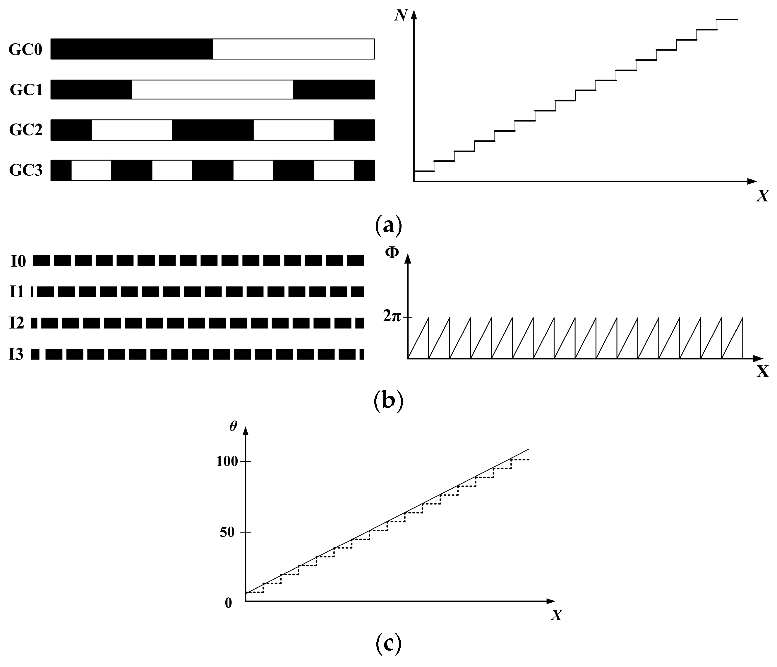
2.2. Light Encoding
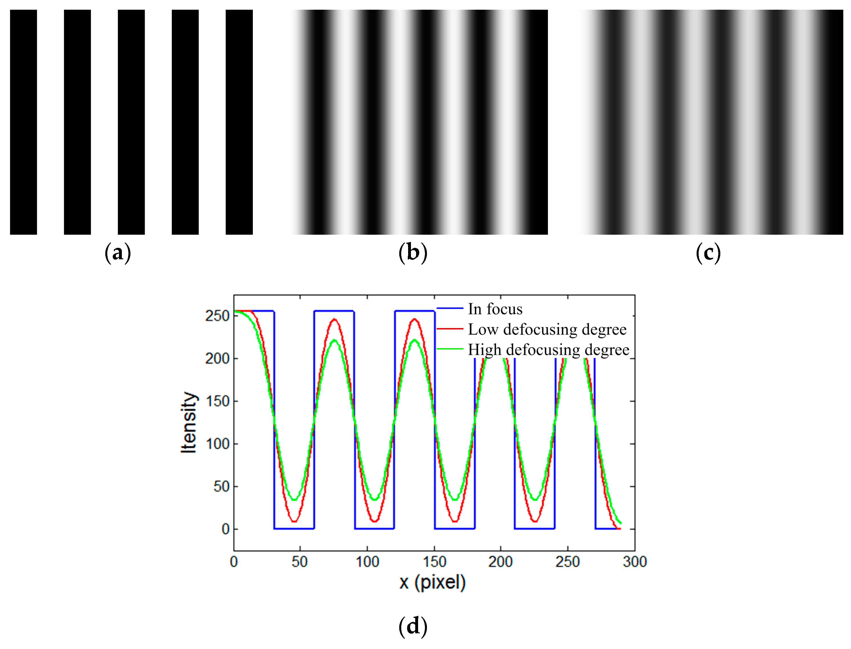
2.3. Digital Binary Defocusing Technique
3. Calibration Principle and Process
3.1. Camera Calibration
3.2. Out-of-Focus Projector Calibration
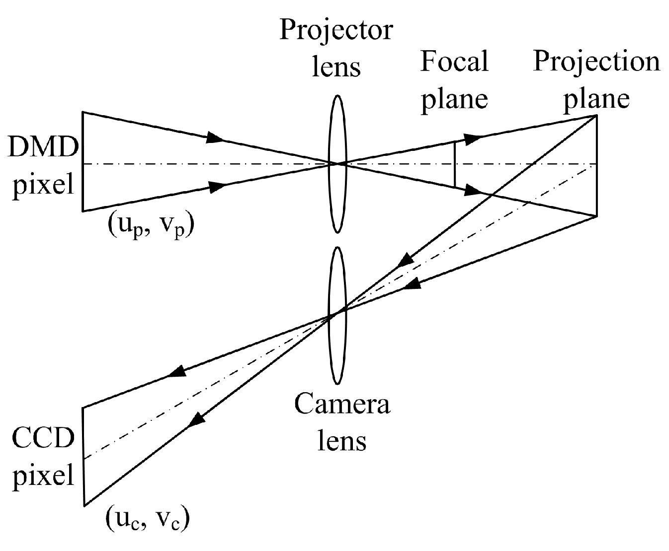
3.2.1. Out-of-Focus Projector Model
3.2.2. Phase-Domain Invariant Mapping
3.3. Out-of-Focus ProjectorCalibration Process
- Step 1:
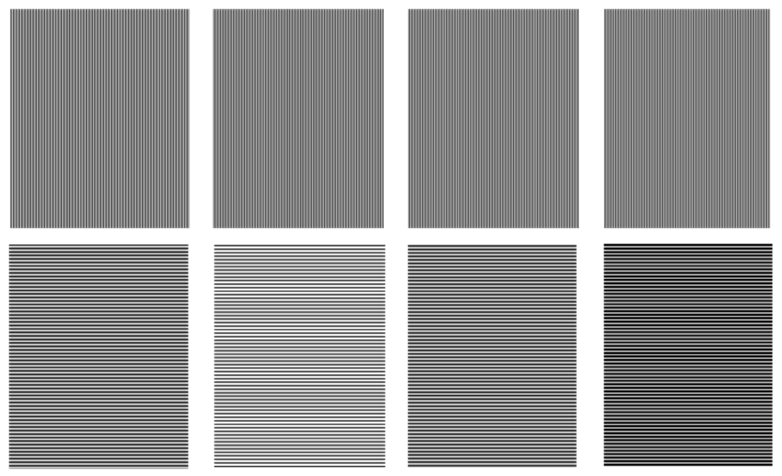
- Image capture. The calibration board was placed on the preset location, and a white paper was stuck on the surface of the calibration board. A set of horizontal and vertical gray code patterns was projected onto the calibration board. These fringe images were captured by the camera. Similarly, the pattern images were captured by projecting a sequence of horizontal and vertical four-step phase shifting fringes. After, the white paper was removed, and the calibration board image was captured. For each pose, a total of 21 images were recorded, which were used to recover the absolute phase using the combination of gray code and the four-step phase shifting algorithm, introduced in Section 2.2.
- Step 2:
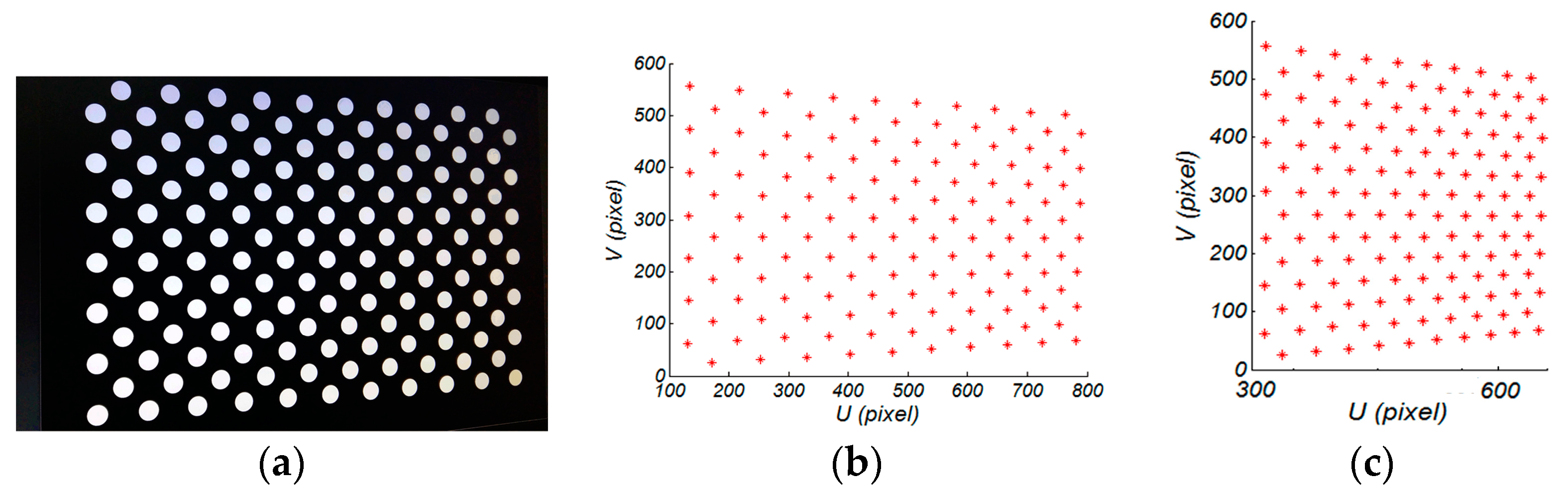
- Camera calibration and determining the location of the circle centers on the DMD. The camera calibration method recommended in Section 3.1 was used. For each calibration pose, the horizontal and vertical absolute phase maps were recovered. A unique point-to-point mapping between CCD and DMD was determined as follows:where is the four-step phase shifting patterns period in the vertical and horizontal directions, respectively. In this paper, pixels. Using Equation (22), the phase value was converted into projector pixels. Furthermore, we assigned the sub-pixel absolute phases, as obtained by the bilinear interpolation of the absolute phases of its four adjacent pixels, because of the sub-pixel circle center detection algorithm for the camera image. For high accuracy camera circle centers, the standard OpenCV toolbox was used. Figure 12 shows an example of the extracted correspondences for a single translation.
- Step 3:
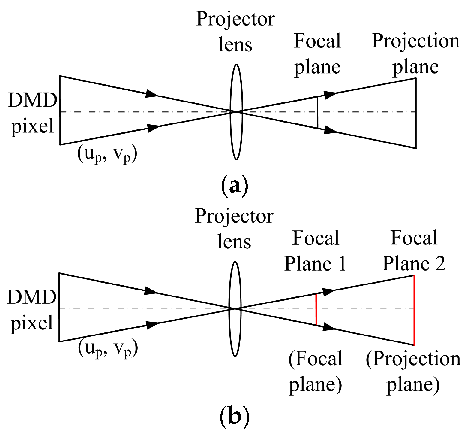
- Calculate the initial values of the intrinsic and extrinsic parameters on the focal plane (focal plane 1). To find approximate parameters, 15 different positions and orientation (poses) images were captured within the scheme measurement volume for the projector calibration. If the reference calibration data on focal plane 1 for the projector were extracted from Step 2, the coarse intrinsic and extrinsic parameters of an out-of-focus projector can be estimated using the same software algorithms for camera calibration on focal plane 1, which was described in Section 3.2.
- Step 4:
- Compute the initial value of the lens distortion on the projection plane. According to the results of our previous experiments in Section 3.2.1, the lens distortion varies with an increasing defocusing degree. To find the approximate parameters, the lens distortion on the projection plane was considered as the initial value of the lens distortion for an out-of-focus projector. In this process, the projector was adjusted to focus on the projection plane, which was called focal plane 2. With the calibration points on focal plane 2 and their corresponding image points on the DMD, the lens distortion on the projection plane was obtained using the pinhole camera model.
- Step 5:
- Compute the precise calibration parameters of the out-of-focus projector by using a nonlinear optimization algorithm. All of the parameters were solved by minimizing the following cost function, as outlined in Equation (20).
4. Experiment and Discussion
5. Conclusions
Acknowledgments
Author Contributions
Conflicts of Interest
References
- Chen, F.; Brown, G.M.; Song, M. Overview of three-dimensional shape measurement using optical methods. Opt. Eng. 2000, 39, 10–22. [Google Scholar]
- D’Apuzzo, N. Overview of 3D surface digitization technologies in Europe. In Proceedings of the SPIE Electronic Imaging, San Jose, CA, USA, 26 January 2006; pp. 605–613. [Google Scholar]
- Abdel-Aziz, Y.I.; Karara, H.M.; Hauck, M. Direct Linear Transformation from Comparator Coordinates into Object Space Coordinates in Close-Range Photogrammetry. Photogramm. Eng. Remote Sens. 2015, 81, 103–107. [Google Scholar] [CrossRef]
- Faig, W. Calibration of close-range photogrammetry systems: Mathematical formulation. Photogramm. Eng. Remote Sens. 1975, 41, 1479–1486. [Google Scholar]
- Tsai, R. A versatile camera calibration technique for high-accuracy 3D machine vision metrology using off-the-shelf TV cameras and lenses. IEEE J. Robot. Autom. 1987, 3, 323–344. [Google Scholar] [CrossRef]
- Luong, Q.-T.; Faugeras, O.D. Self-Calibration of a Moving Camera from PointCorrespondences and Fundamental Matrices. Int. J. Comput. Vis. 1997, 22, 261–289. [Google Scholar] [CrossRef]
- Zhang, Z.Y. Flexible camera calibration by viewing a plane from unknown orientations. In Proceedings of the IEEE Conference on Computer Vision, Corfu, Greece, 20–27 September 1999; pp. 666–673. [Google Scholar]
- Qi, Z.H.; Xiao, L.X.; Fu, S.H.; Li, T.; Jiang, G.W.; Long, X.J. Two-Step Camera Calibration Method Based on the SPGD Algorithm. Appl. Opt. 2012, 51, 6421–6428. [Google Scholar] [CrossRef] [PubMed]
- Bacakoglu, H.; Kamel, M. An Optimized Two-Step Camera Calibration Method. In Proceedings of the IEEE International Conference on Robotics and Automation, Albuquerque, NM, USA, 25 April 1997; pp. 1347–1352. [Google Scholar]
- Huang, L.; Zhang, Q.C.; Asundi, A. Camera Calibration with Active Phase Target: Improvement on Feature Detection and Optimization. Opt. Lett. 2013, 38, 1446–1448. [Google Scholar] [CrossRef] [PubMed]
- Jia, Z.Y.; Yang, J.H.; Liu, W.; Wang, F.J.; Liu, Y.; Wang, L.L.; Fan, C.N.; Zhao, K. Improved Camera Calibration Method Based on Perpendicularity Compensation for Binocular Stereo Vision Measurement System. Opt. Express 2015, 23, 15205–15223. [Google Scholar] [CrossRef] [PubMed]
- Zhu, F.P.; Shi, H.J.; Bai, P.X.; Lei, D.; He, X.Y. Nonlinear Calibration for Generalized Fringe Projection Profilometry under Large Measuring Depth Range. Appl. Opt. 2013, 52, 7718–7723. [Google Scholar] [CrossRef] [PubMed]
- Huang, L.; Chua, P.S.K.; Asundi, A. Least-squares calibration method for fringe projection profilometry considering camera lens distortion. Appl. Opt. 2010, 49, 1539–1548. [Google Scholar] [CrossRef] [PubMed]
- Lu, J.; Mo, R.; Sun, H.B.; Chang, Z.Y. Flexible Calibration of Phase-to-Height Conversion in Fringe Projection Profilometry. Appl. Opt. 2016, 55, 6381–6388. [Google Scholar] [CrossRef] [PubMed]
- Zhang, X.; Zhu, L.M. Projector calibration from the camera image point of view. Opt. Eng. 2009, 48, 208–213. [Google Scholar] [CrossRef]
- Gao, W.; Wang, L.; Hu, Z.Y. Flexible Method for Structured Light System Calibration. Opt. Eng. 2008, 47, 767–781. [Google Scholar] [CrossRef]
- Huang, Z.R.; Xi, J.T.; Yu, Y.G.; Guo, Q.H. Accurate projector calibration based on a new point-to-point mapping relationship between the camera and projector images. Appl. Opt. 2015, 54, 347–356. [Google Scholar] [CrossRef]
- Huang, J.; Wang, Z.; Gao, J.M.; Xue, Q. Projector calibration with error surface compensation method in the structured light three-dimensional measurement system. Opt. Eng. 2013, 52, 043602. [Google Scholar] [CrossRef]
- Moreno, D.; Taubin, G. Simple, Accurate, and Robust Projector-Camera Calibration. In Proceedings of the 2012 IEEE Second International Conference on 3D Imaging, Modeling, Processing, Visualization and Transmission, Zurich, Switzerland, 13–15 October 2012; pp. 464–471. [Google Scholar]
- Chen, R.; Xu, J.; Chen, H.P.; Su, J.H.; Zhang, Z.H.; Chen, K. Accurate Calibration Method for Camera and Projector in Fringe Patterns Measurement System. Appl. Opt. 2016, 55, 4293–4300. [Google Scholar] [CrossRef] [PubMed]
- Liu, M.; Sun, C.K.; Huang, S.J.; Zhang, Z.H. An Accurate Projector Calibration Method Based on Polynomial Distortion Representation. Sensors 2015, 15, 26567–26582. [Google Scholar] [CrossRef] [PubMed]
- Yang, S.R.; Liu, M.; Song, J.H.; Yin, S.B.; Guo, Y.; Ren, Y.J.; Zhu, J.G. Flexible Digital Projector Calibration Method Based on Per-Pixel Distortion Measurement and Correction. Opt. Lasers Eng. 2017, 92, 29–38. [Google Scholar] [CrossRef]
- Gong, Y.Z.; Zhang, S. Ultrafast 3-D shape measurement with an Off-the-shelf DLP projector. Opt. Express 2010, 18, 19743–19754. [Google Scholar] [CrossRef] [PubMed]
- Karpinsky, N.; Zhang, S. High-resolution, real-time 3D imaging with fringe analysis. J. Real-Time Image Process. 2012, 7, 55–66. [Google Scholar] [CrossRef]
- Zhang, S. Recent progresses on real-time 3D shape measurement using digital fringe projection techniques. Opt. Lasers Eng. 2010, 48, 149–158. [Google Scholar] [CrossRef]
- Lei, S.; Zhang, S. Flexible 3-D shape measurement using projector defocusing. Opt. Lett. 2009, 34, 3080–3082. [Google Scholar] [CrossRef] [PubMed]
- Lei, S.; Zhang, S. Digital sinusoidal fringe pattern generation: Defocusing binary patterns VS focusing sinusoidal patterns. Opt. Lasers Eng. 2010, 48, 561–569. [Google Scholar] [CrossRef]
- Merner, L.; Wang, Y.; Zhang, S. Accurate calibration for 3D shape measurement system using a binary defocusing technique. Opt. Lasers Eng. 2013, 51, 514–519. [Google Scholar] [CrossRef]
- Li, B.; Karpinsky, N.; Zhang, S. Novel calibration method for structured-light system with an out-of-focus projector. Appl. Opt. 2014, 53, 3415–3426. [Google Scholar] [CrossRef] [PubMed]
- Weng, J.Y.; Cohen, P.; Herniou, M. Calibration of Stereo Cameras Using a Non-Linear Distortion Model. In Proceedings of the Tenth International Conference on Pattern Recognition, Atlantic City, NJ, USA, 16–21 June 1990; pp. 246–253. [Google Scholar]
- Faisal, B.; Matthew, N.D. Automatic Radial Distortion Estimation from a Single Image. J. Math. Imaging Vis. 2013, 45, 31–45. [Google Scholar]
- Hartley, R.I.; Tushar, S. The Cubic Rational Polynomial Camera Model. Image Underst. Workshop 1997, 649, 653. [Google Scholar]
- Claus, D.; Fitzgibbon, A.W. A Rational Function Lens Distortion Model for General Cameras. In Proceedings of the IEEE Computer Society Conference on Computer Vision and Pattern Recognition, San Diego, CA, USA, 20–25 June 2005; pp. 213–219. [Google Scholar]
- Santana-Cedrés, D.; Gómez, L.; Alemán-Flores, M.; Agustín, S.; Esclarín, J.; Mazorra, L.; Álvarez, L. An Iterative Optimization Algorithm for Lens Distortion Correction Using Two-Parameter Models. SIAM J. Imaging Sci. 2015, 8, 1574–1606. [Google Scholar] [CrossRef]
- Tang, Z.W.; von Gioi Grompone, R.; Monasse, P.; Morel, J.M. A Precision Analysis of Camera Distortion Models. IEEE Trans. Image Process. 2017, 26, 2694–2704. [Google Scholar] [CrossRef] [PubMed]
- Salvi, J.; Pagès, J.; Batlle, J. Pattern codification strategies in structured light systems. Pattern Recognit. 2004, 37, 827–849. [Google Scholar] [CrossRef]
- Sansoni, G.; Carocci, M.; Rodella, R. Three-dimensional vision based on a combination of gray-code and phase-shift light projection: Analysis and compensation of the systematic errors. Appl. Opt. 1999, 38, 6565–6573. [Google Scholar] [CrossRef] [PubMed]
- Stokseth, P.A. Properties of a Defocused Optical System. J. Opt. Soc. Am. 1969, 59, 1314–1321. [Google Scholar] [CrossRef]
- Wang, Y.J.; Zhang, S. Comparison of the Squared Binary, Sinusoidal Pulse Width Modulation, and Optimal Pulse Width Modulation Methods for Three-Dimensional Shape Measurement with Projector Defocusing. Appl. Opt. 2012, 51, 861–872. [Google Scholar] [CrossRef] [PubMed]
- Chao, Z.; Chen, Q.; Feng, S.J.; Feng, F.X.Y.; Gu, G.H.; Sui, X.B. Optimized Pulse Width Modulation Pattern Strategy for Three-Dimensional Profilometry with Projector Defocusing. Appl. Opt. 2012, 51, 4477–4490. [Google Scholar]
- Wang, Y.J.; Zhang, S. Optimal Pulse Width Modulation for Sinusoidal Fringe Generation with Projector Defocusing. Opt. Lett. 2010, 35, 4121–4123. [Google Scholar] [CrossRef] [PubMed]
- Gastón, A.A.; Jaime, A.A.; J. Matías, D.M.; José, A.F. Pulse-Width Modulation in Defocused Three-Dimensional Fringe Projection. Opt. Lett. 2010, 35, 3682–3684. [Google Scholar]
- Wang, Y.J.; Zhang, S. Three-Dimensional Shape Measurement with Binary Dithered Patterns. Appl. Opt. 2012, 51, 6631–6636. [Google Scholar] [CrossRef] [PubMed]
- Moré, J.J. The Levenberg-Marquardt Algorithm: Implementation and Theory. In Proceedings of the Numerical Analysis: Proceedings of the Biennial Conference, Dundee, UK, 28 June–1 July 1977; pp. 105–116. [Google Scholar]
- Srikanth, M.; Krishnan, K.S.G.; Sowmya, V.; Soman, K.P. Image Denoising Based on Weighted Regularized Least Square Method. In Proceedings of the International Conference on Circuit, Power and Computing Technologies (ICCPCT), Kollam, India, 20–21 April 2017; pp. 1–5. [Google Scholar]


| Defocusing Degree | Re-Projection Errors | |||||
|---|---|---|---|---|---|---|
| 1 | 2033.15992 | 481.85752 | −0.00501 | 0.00741 | 0.02071 | 0.03627 |
| 2029.32333 | 794.04516 | 0.10553 | −0.00781 | |||
| 2 | 2066.07579 | 480.66343 | 0.00025 | 0.00075 | 0.02356 | 0.04631 |
| 2060.38058 | 817.00819 | −0.02750 | −0.00774 | |||
| 3 | 2066.02355 | 482.08093 | −0.01202 | −0.00303 | 0.02856 | 0.05781 |
| 2061.98782 | 824.49272 | −0.01985 | −0.00817 | |||
| 4 | 2083.24450 | 457.53174 | −0.03166 | −0.00456 | 0.03862 | 0.07487 |
| 2079.93614 | 834.40594 | 0.08715 | −0.01328 | |||
| 5 | 2082.66646 | 458.68461 | −0.09894 | −0.01726 | 0.05492 | 0.09577 |
| 2090.35224 | 801.22181 | 0.13975 | −0.01243 | |||
| Defocusing Degree | Re-Projection Errors | |||||
|---|---|---|---|---|---|---|
| 1 | 2065.84461 | 486.73708 | 0.00832 | −0.00052 | 0.02950 | 0.03762 |
| 2068.06661 | 815.66697 | −0.03886 | −0.00749 | |||
| 2 | 2074.79015 | 503.27888 | 0.00111 | 0.00496 | 0.03941 | 0.05078 |
| 2074.45555 | 824.02444 | 0.03516 | −0.00402 | |||
| 3 | 2131.24929 | 526.11764 | 0.00240 | −0.00229 | 0.05352 | 0.07076 |
| 2135.41564 | 799.98280 | 0.03484 | −0.00229 | |||
| 4 | 2165.81230 | 541.55585 | −0.02157 | −0.00543 | 0.07101 | 0.09316 |
| 2166.67073 | 794.56998 | 0.17737 | 0.00042 | |||
| 5 | 2173.40017 | 531.46318 | 0.01313 | −0.00125 | 0.09358 | 0.14790 |
| 2172.43898 | 810.09141 | 0.10122 | −0.00151 | |||
| Statistic | Defocusing Degree | ||||
|---|---|---|---|---|---|
| 1 | 2 | 3 | 4 | 5 | |
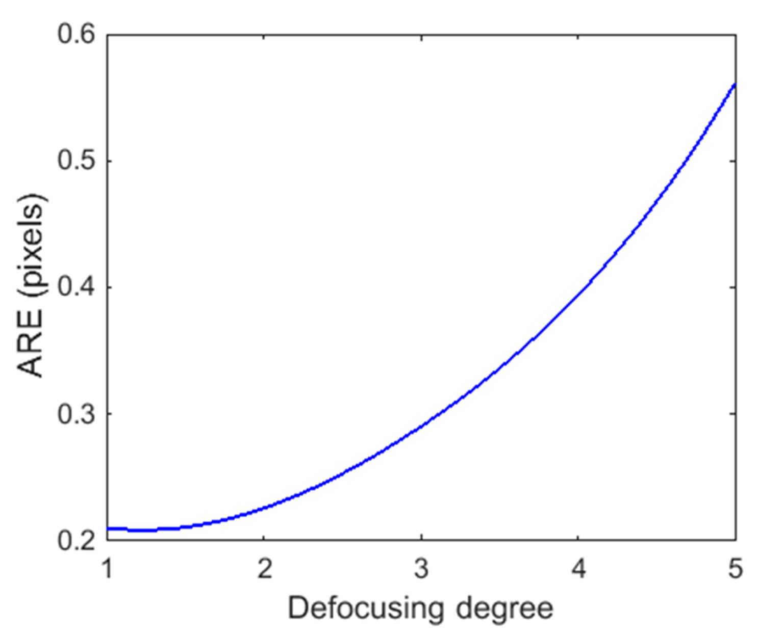
| ARE | 0.21043 | 0.22585 | 0.29015 | 0.39374 | 0.56108 |
| Method | Device | ||||||||
|---|---|---|---|---|---|---|---|---|---|
| Proposed method | Camera | 2708.93985 | 684.18114 | −0.01640 | 0.00698 | 0.94231 −0.01042 −0.25359 | −0.00342 0.99926 −0.00936 | 0.23016 0.00653 0.73162 | −389.37651 179. 73663 229.32452 |
| 2732.74604 | 740.39548 | 0.03143 | −0.00944 | ||||||
| Projector | 2065.25354 | 461.4964 | −0.06638 | −0.00567 | |||||
| 2061.88752 | 798.62552 | 0.02323 | −0.00562 | ||||||
| The method in [29] | Camera | 2708.93865 | 684.16035 | −0.01640 | 0.00698 | 0.94242 −0.01038 −0.25338 | 0.00364 0.99952 −0.00929 | 0.23024 0.00681 0.73139 | −389.35619 180.0085 230.02781 |
| 2732.74653 | 740.39749 | 0.03143 | −0.00944 | ||||||
| Projector | 2066.07579 | 480.66343 | 0.00025 | 0.00075 | |||||
| 2060.38058 | 817.00819 | −0.02750 | −0.00774 | ||||||
| Statistic | Defocusing Degree | Mean | SD | Max. |
|---|---|---|---|---|
| Plane by CMM | Null | 0.0065 | 0.0085 | 0.0264 |
| Plane by camera-projector system with our proposed projector calibration method | 1 | 0.0138 | 0.0168 | 0.0620 |
| 2 | 0.0147 | 0.0184 | 0.0837 | |
| 3 | 0.0159 | 0.0195 | 0.0853 | |
| 4 | 0.0162 | 0.0208 | 0.0864 | |
| 5 | 0.0172 | 0.0234 | 0.0882 | |
| Plane by camera-projector system with the proposed projector calibration method in [29] | 1 | 0.0138 | 0.0168 | 0.0620 |
| 2 | 0.0169 | 0.0210 | 0.0889 | |
| 3 | 0.0183 | 0.0257 | 0.0895 | |
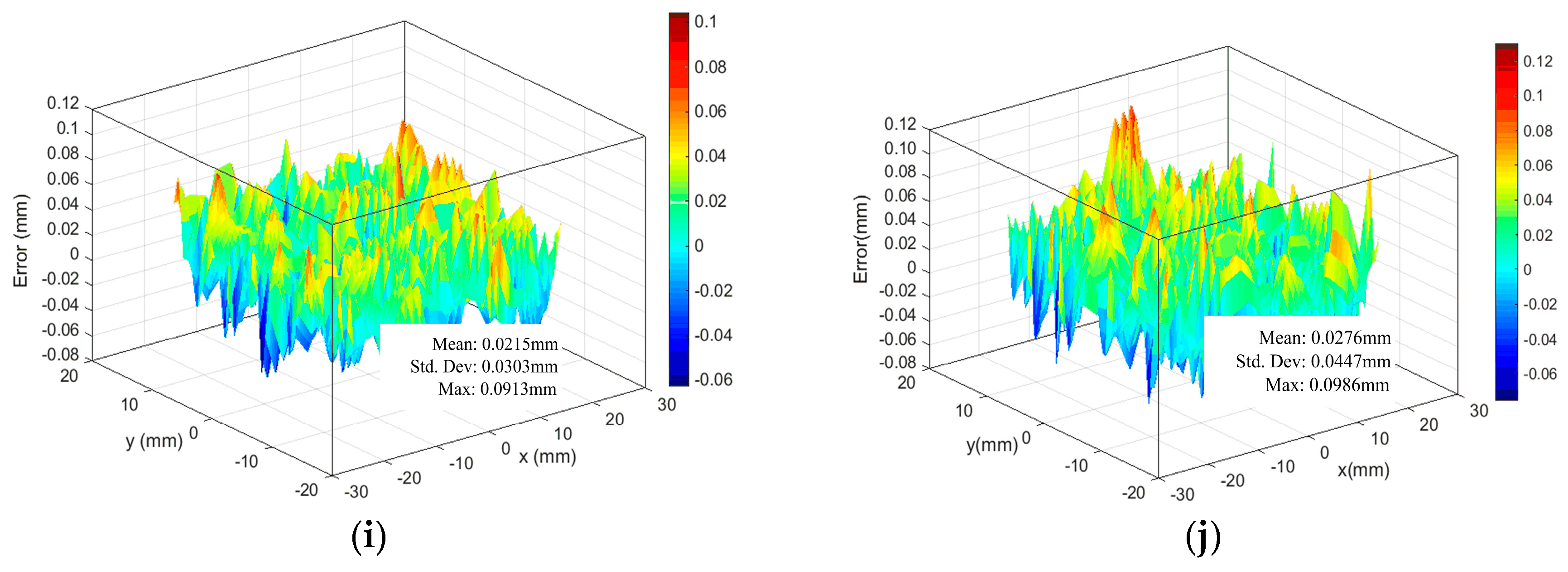
| 4 | 0.0215 | 0.0303 | 0.0913 | |
| 5 | 0.0276 | 0.0447 | 0.0986 |
| Statistic | Defocusing Degree | Fitting Radius | Mean | SD | Max. |
|---|---|---|---|---|---|
| Hemisphere by CMM | Null | 20.0230 | 0.0204 | 0.0473 | 0.1165 |
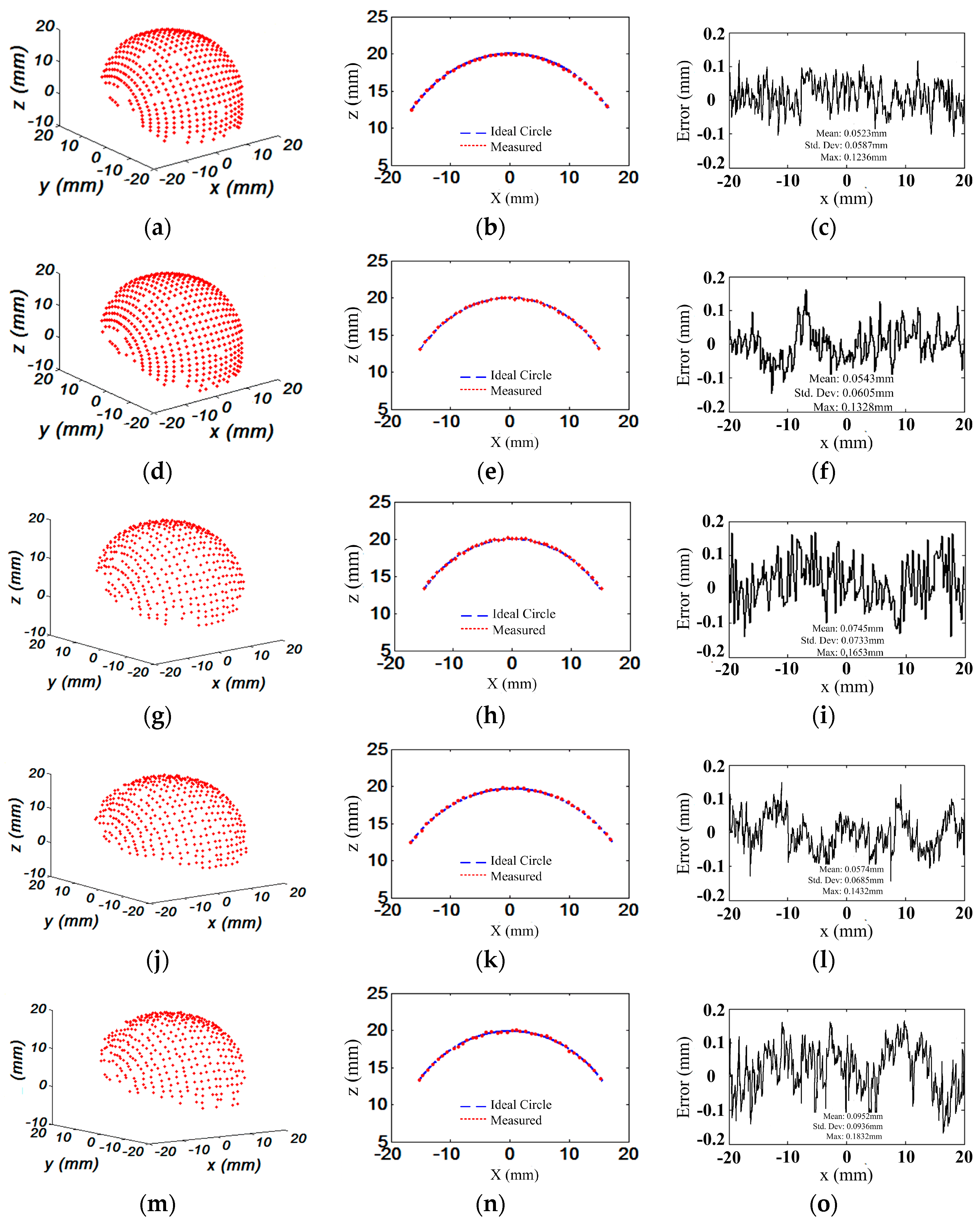
| Hemisphere by camera-projector system with our proposed projector calibration method | 1 | 19.9745 | 0.0523 | 0.0587 | 0.1236 |
| 2 | 19.9542 | 0.0543 | 0.0605 | 0.1328 | |
| 5 | 19.9537 | 0.0574 | 0.0685 | 0.1432 | |
| Hemisphere by camera-projector system with the proposed projector calibration method in [29] | 1 | 19.9745 | 0.0523 | 0.0587 | 0.1236 |
| 2 | 19.9358 | 0.0745 | 0.0733 | 0.1653 | |
| 5 | 19.9108 | 0.0952 | 0.0936 | 0.1832 |
© 2017 by the authors. Licensee MDPI, Basel, Switzerland. This article is an open access article distributed under the terms and conditions of the Creative Commons Attribution (CC BY) license (http://creativecommons.org/licenses/by/4.0/).
Share and Cite
Zhang, J.; Zhang, Y.; Chen, B. Out-of-Focus Projector Calibration Method with Distortion Correction on the Projection Plane in the Structured Light Three-Dimensional Measurement System. Sensors 2017, 17, 2963. https://doi.org/10.3390/s17122963
Zhang J, Zhang Y, Chen B. Out-of-Focus Projector Calibration Method with Distortion Correction on the Projection Plane in the Structured Light Three-Dimensional Measurement System. Sensors. 2017; 17(12):2963. https://doi.org/10.3390/s17122963
Chicago/Turabian StyleZhang, Jiarui, Yingjie Zhang, and Bo Chen. 2017. "Out-of-Focus Projector Calibration Method with Distortion Correction on the Projection Plane in the Structured Light Three-Dimensional Measurement System" Sensors 17, no. 12: 2963. https://doi.org/10.3390/s17122963