
A Versatile and Reproducible Multi-Frequency Electrical Impedance Tomography System


Abstract
:
1. Introduction
1.1. Electrical Impedance Tomography
1.2. EIT Hardware
1.3. EIT Applications
1.4. Purpose
- Parallel recording of all voltages for processing of data “offline”, allowing for additional signals, such as EEG/ECoG to be recorded alongside the EIT signal.
- Noise, frame rate and performance characteristics comparable to existing EIT systems. Target resistance changes of ≈0.1% have been previously identified for EIT recordings of fast neural activity related to neuronal depolarization and scalp recordings of epilepsy [6,16]. This requires stable current injection, <0.1% noise, and voltage recording with accuracy of ≈100 nV.
- Variable electrode count, up to a maximum of 256 electrodes.
- Ability to synchronise injection/recording with external triggers (whisker stimulation, visual, auditory). The phase of injected current should be randomised with respect to the stimulation, to minimise the phase related artefacts in EP recordings [28].
- Reconfigurable modes of operation, to allow for new functionality to be introduced as a later date. Ideally, this should be achievable through software or firmware changes only.
- Easily reproducible. Currently, construction of a non-commercial EIT system can take several months and existing publications on EIT systems typically lack enough detail to allow replication. A system which can be easily replicated using a mixture of off the shelf equipment, alongside open source software and hardware designs, will significantly reduce the workload and allow new systems to be assembled in a matter of weeks.
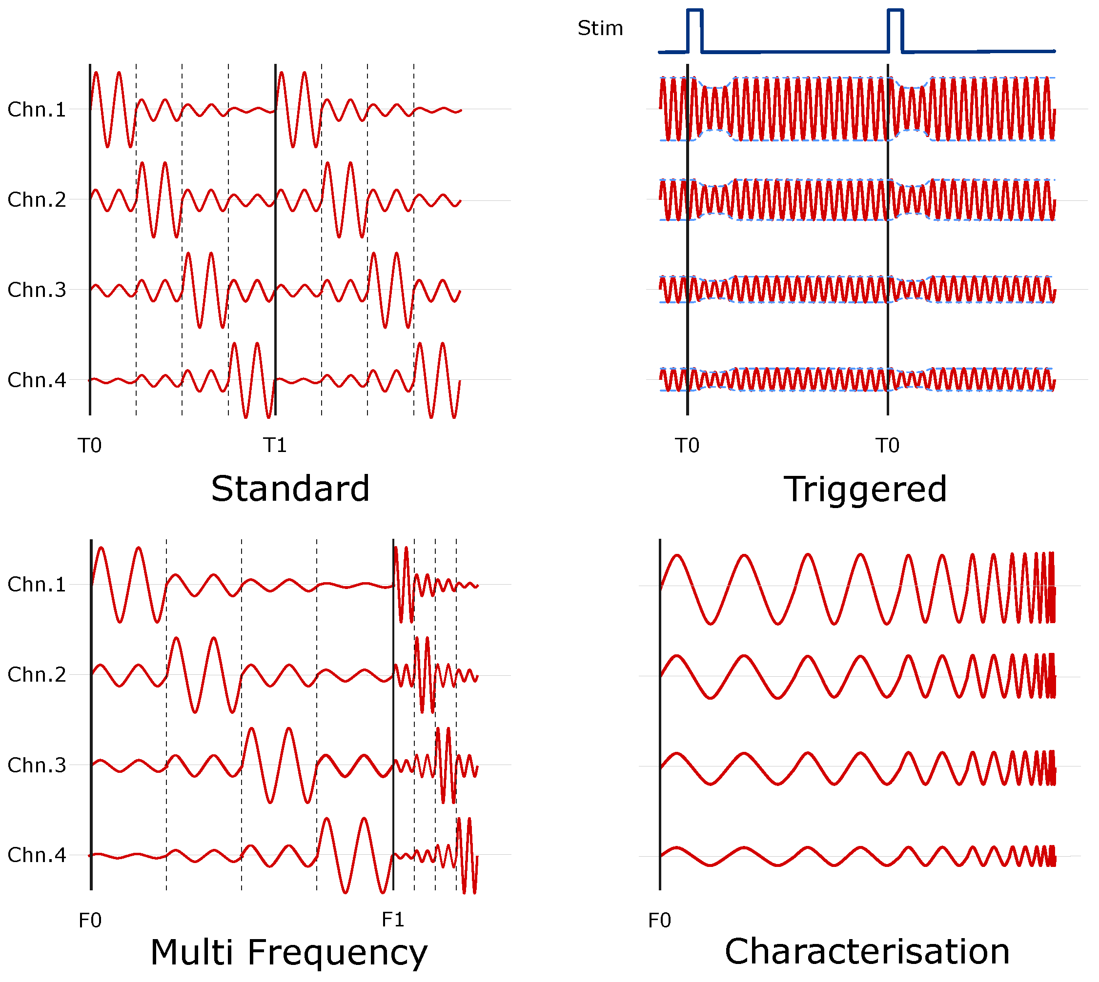
1.5. Experimental Design
2. Materials and Methods
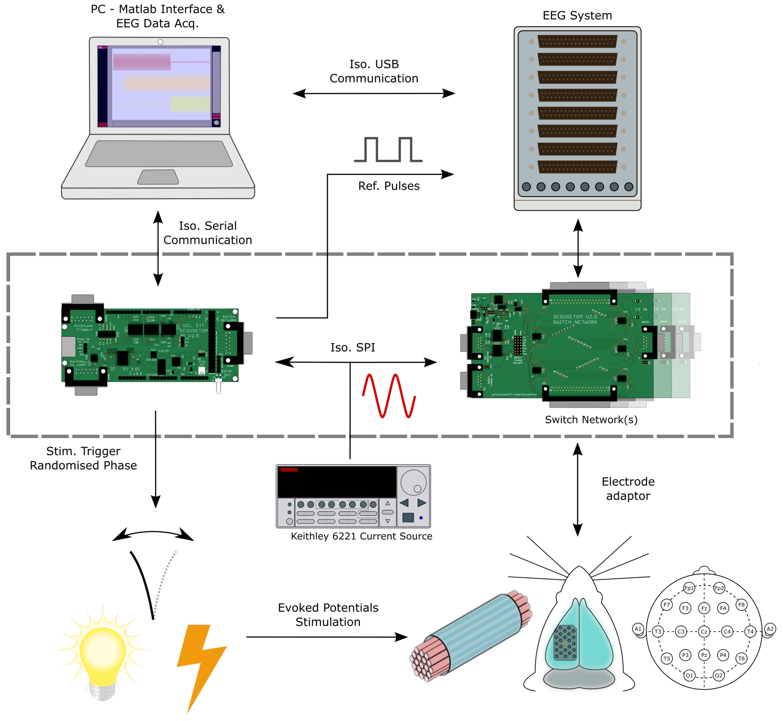
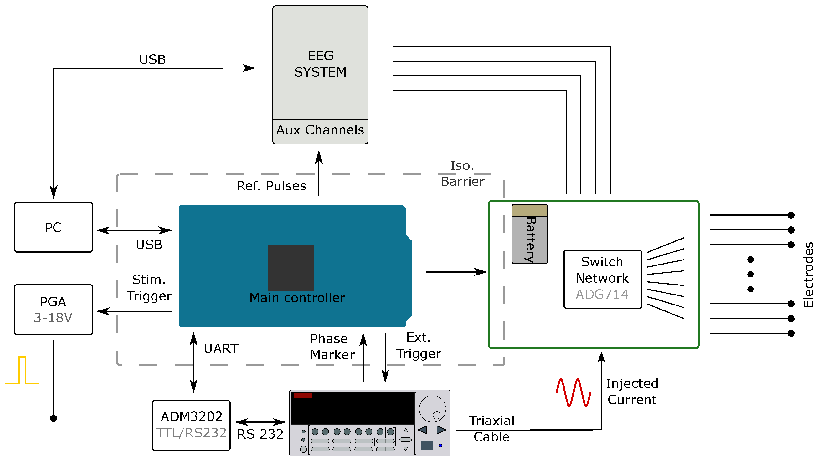
2.1. System Design
2.1.1. Current Source
2.1.2. Voltage Recording
2.1.3. Controller and Switch Network
2.1.4. Controller Software
2.1.5. Data Processing Software
2.1.6. Electrode Connectors
2.2. System Characterisation
2.2.1. Resistor Phantom—Noise & Drift
2.2.2. Resistor Phantom—Frequency Response
2.3. Experimental Data
2.3.1. Scalp Recordings—Preparation
2.3.2. EIT Reconstruction
2.3.3. Time Difference—Imaging Haemorrhage
2.3.4. Time Difference—Scalp Recordings
2.3.5. Triggered Averaging—Rat Somatosensory Cortex
2.3.6. Multifrequency—Scalp Recordings
2.3.7. Impedance Spectrum Characterisation—Ischaemic Rat Brain
2.4. Data Presentation
3. Results
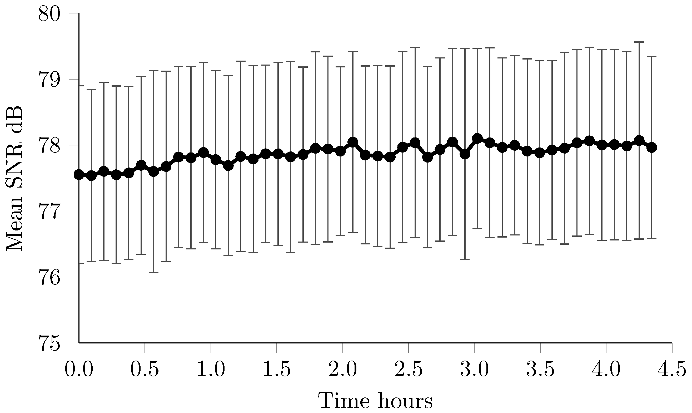
3.1. Resistor Phantom—Noise & Drift
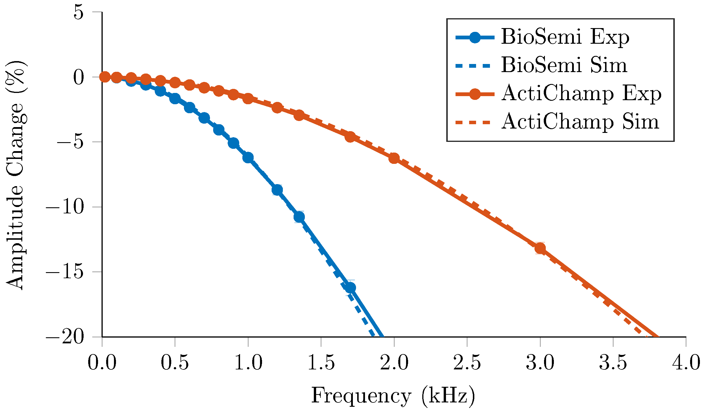
3.2. Resistor Phantom—Frequency Response
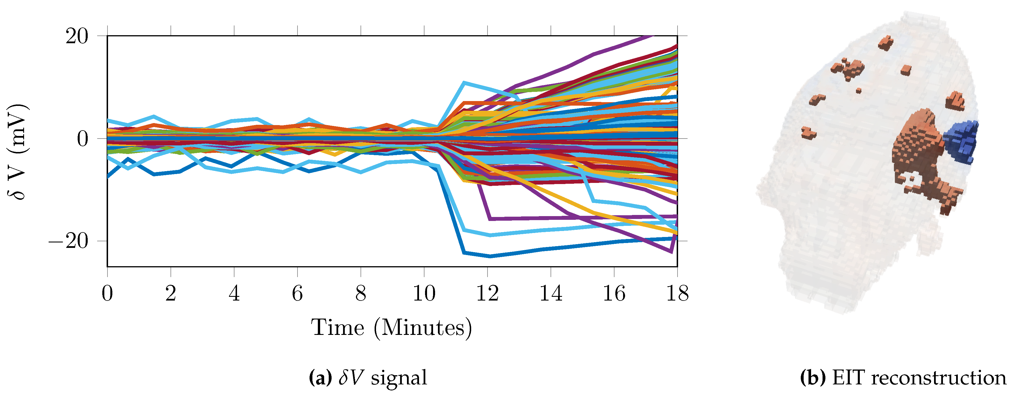
3.3. Time Difference—Imaging Haemorrhage
3.4. Time Difference—Scalp Recordings
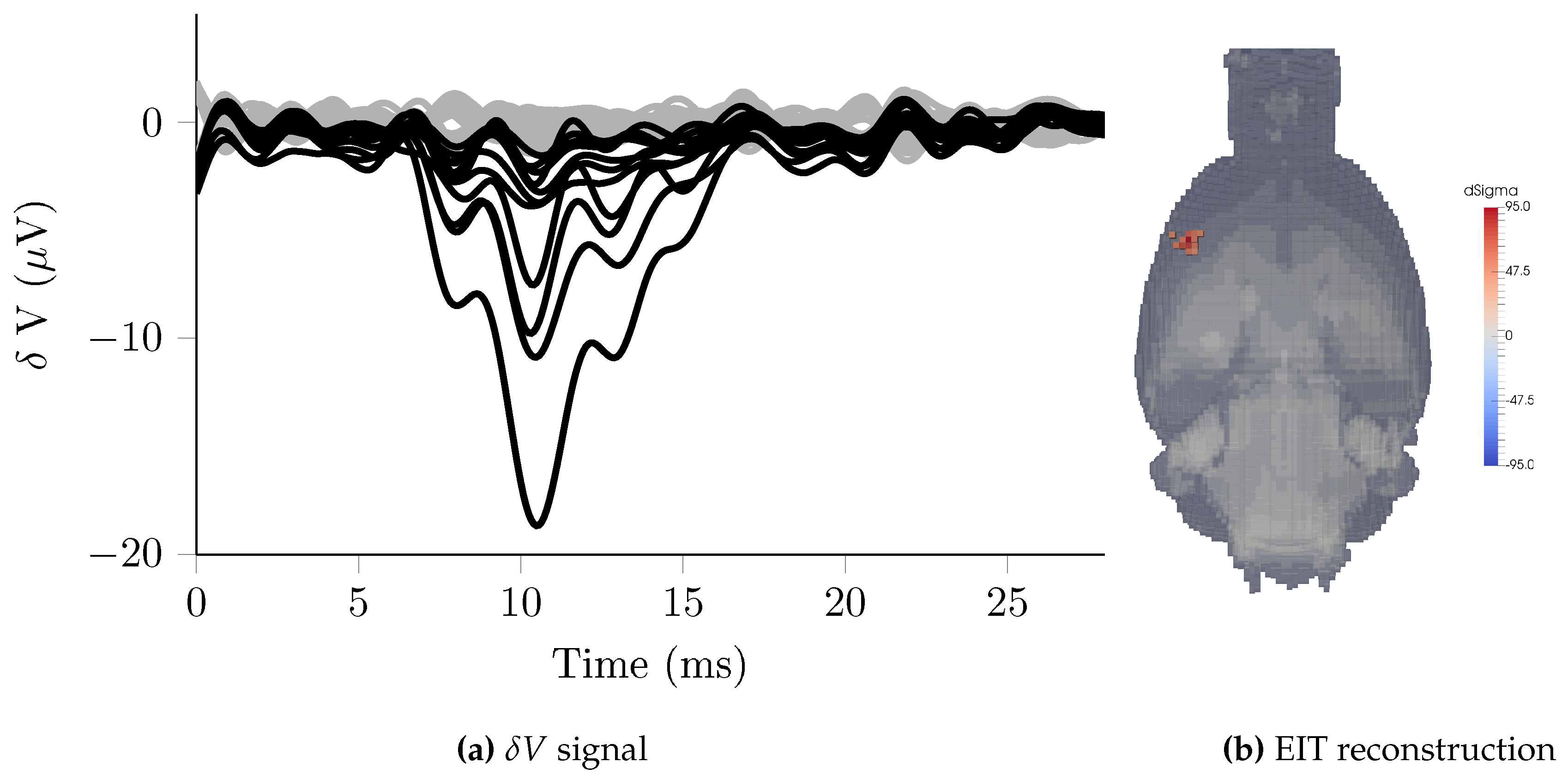
3.5. Triggered Averaging—Rat Somatosensory Cortex
3.6. Multifrequency—Scalp Recordings
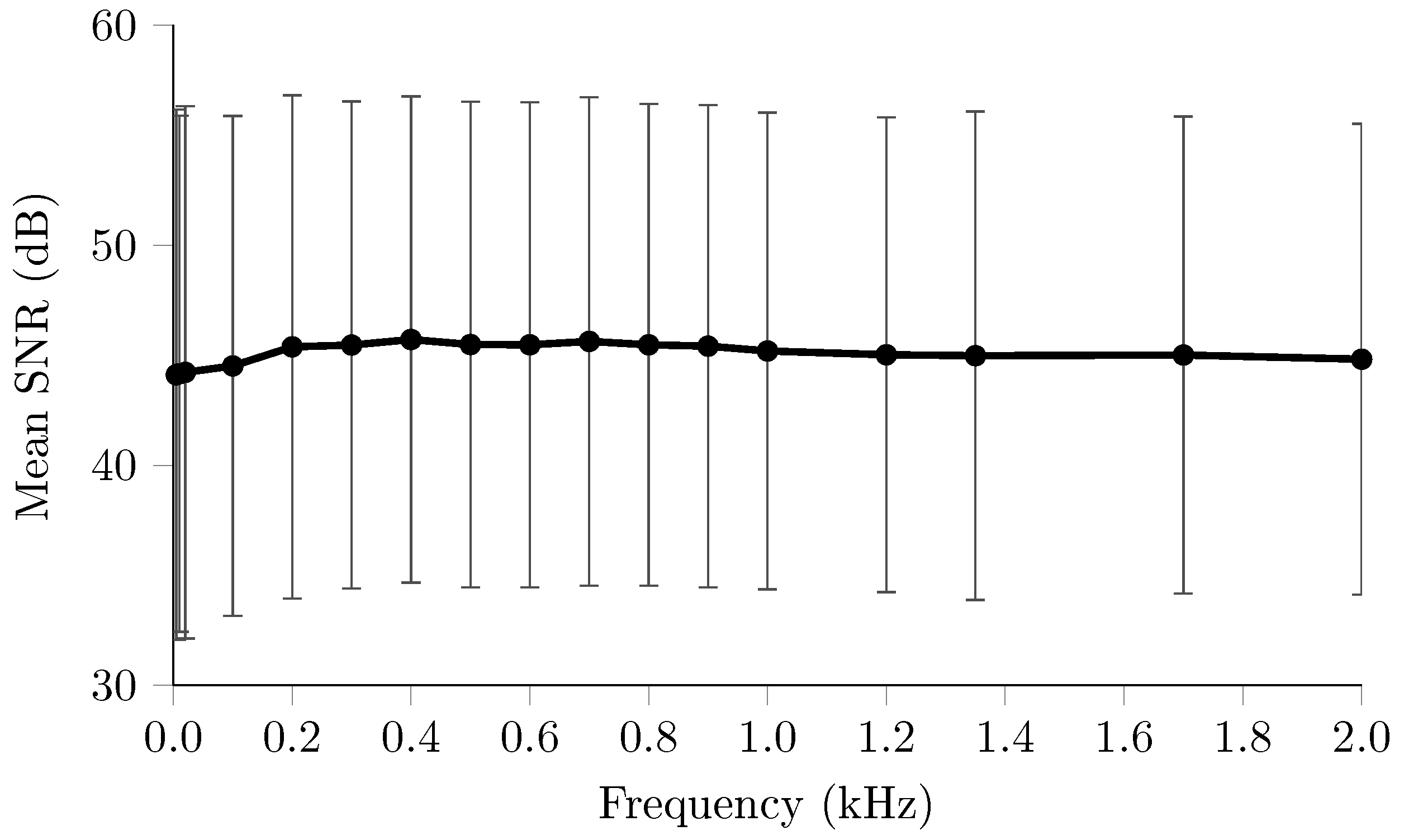
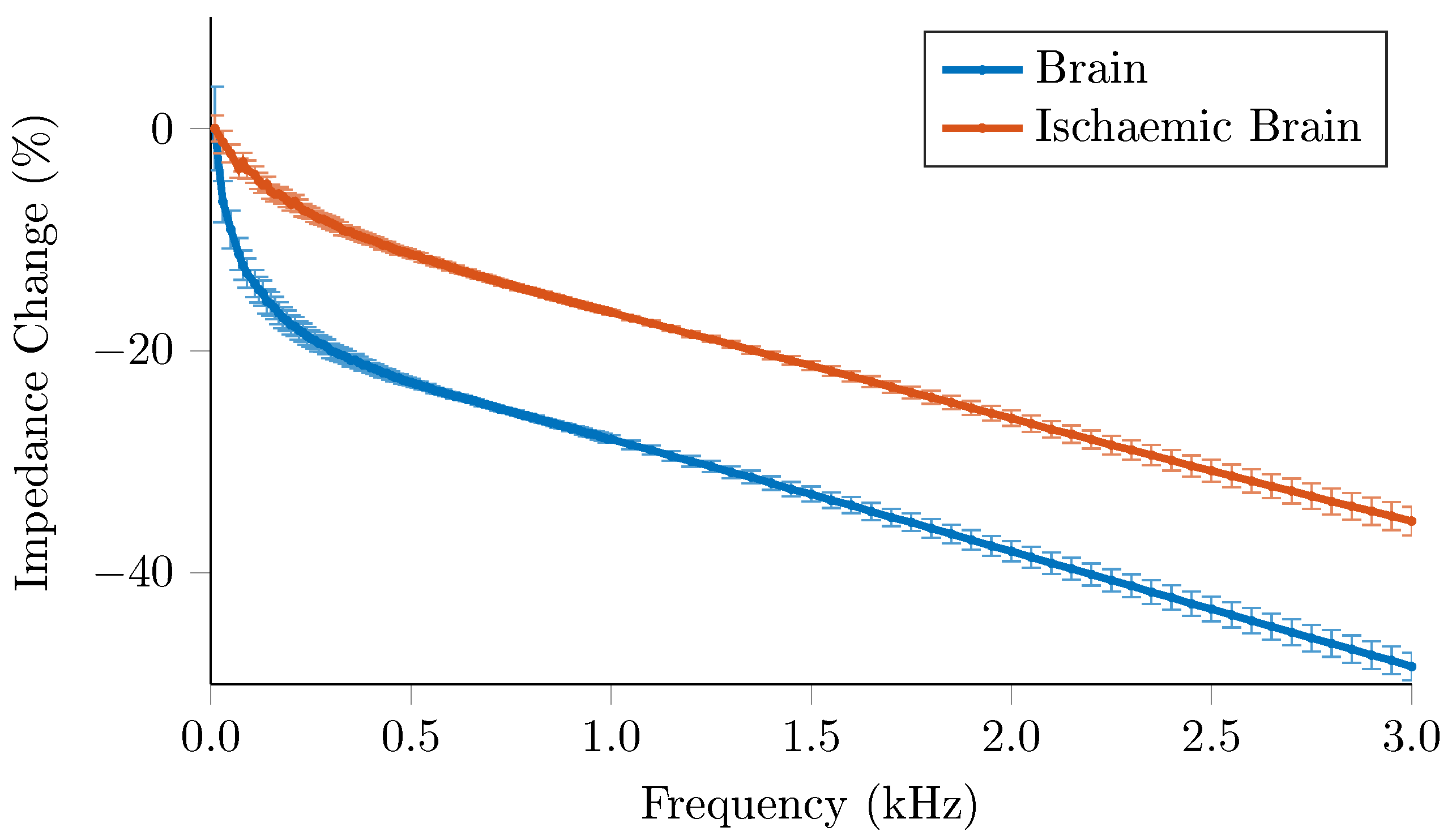
3.7. Impedance Spectrum Measurement
4. Discussion
4.1. System Characterisation
4.2. Time Difference
4.3. Triggered Averaging
4.4. Multifrequency
4.5. Characterisation
4.6. Design Criteria and Technical Limitations
4.7. Reproducibility and Recommendations for Use
5. Conclusions
Acknowledgments
Author Contributions
Conflicts of Interest
Appendix A. Hardware & Software Resources
References
- Metherall, P.; Barber, D.; Smallwood, R.; Brown, B. Three dimensional electrical impedance tomography. Nature 1996, 380, 509–512. [Google Scholar] [CrossRef] [PubMed]
- Frerichs, I. Electrical impedance tomography (EIT) in applications related to lung and ventilation: A review of experimental and clinical activities. Physiol. Meas. 2000, 21, R1–R21. [Google Scholar] [CrossRef] [PubMed]
- You, F.; Shuai, W.; Shi, X.; Fu, F.; Liu, R.; Dong, X. In vivo Monitoring by EIT for the Pig’s Bleeding after Liver Injury. In World Congress on Medical Physics and Biomedical Engineering, September 7–12, 2009, Munich, Germany: Vol. 25/2 Diagnostic Imaging; Dössel, O., Schlegel, W.C., Eds.; Springer: Berlin/Heidelberg, Germany, 2009; pp. 110–112. [Google Scholar]
- Halter, R.J.; Hartov, A.; Paulsen, K.D. A broadband high-frequency electrical impedance tomography system for breast imaging. IEEE Trans. Biomed. Eng. 2008, 55, 650–659. [Google Scholar] [CrossRef] [PubMed]
- Vongerichten, A.N.; dos Santos, G.S.; Aristovich, K.; Avery, J.; McEvoy, A.; Walker, M.; Holder, D.S. Characterisation and imaging of cortical impedance changes during interictal and ictal activity in the anaesthetised rat. NeuroImage 2016, 124, 813–823. [Google Scholar] [CrossRef] [PubMed]
- Fabrizi, L.; Sparkes, M.; Horesh, L.; Abascal, J.F.P.-J.; McEwan, A.; Bayford, R.H.; Elwes, R.; Binnie, C.D.; Holder, D.S. Factors limiting the application of electrical impedance tomography for identification of regional conductivity changes using scalp electrodes during epileptic seizures in humans. Physiol. Meas. 2006, 27, S163–S174. [Google Scholar] [CrossRef] [PubMed]
- Dowrick, T.; Blochet, C.; Holder, D. In vivo bioimpedance changes during haemorrhagic and ischaemic stroke in rats: Towards 3D stroke imaging using electrical impedance tomography. Physiol. Meas. 2016, 37, 765–784. [Google Scholar] [CrossRef] [PubMed]
- Manwaring, P.K.; Moodie, K.L.; Hartov, A.; Manwaring, K.H.; Halter, R.J. Intracranial electrical impedance tomography: A method of continuous monitoring in an animal model of head trauma. Anesth. Analg. 2013, 117, 866–875. [Google Scholar] [CrossRef] [PubMed]
- Fu, F.; Li, B.; Dai, M.; Hu, S.J.; Li, X.; Xu, C.H.; Wang, B.; Yang, B.; Tang, M.X.; Dong, X.Z.; et al. Use of electrical impedance tomography to monitor regional cerebral edema during clinical dehydration treatment. PLoS ONE 2014, 9, e113202. [Google Scholar] [CrossRef] [PubMed]
- Aristovich, K.Y.; Packham, B.C.; Koo, H.; dos Santos, G.S.; McEvoy, A.; Holder, D.S. Imaging fast electrical activity in the brain with electrical impedance tomography. NeuroImage 2016, 124, 204–213. [Google Scholar] [CrossRef] [PubMed]
- Aristovich, K.; Blochet, C.; Avery, J.; Donega, M.; Holder, D. EIT of evoked and spontaneous activity in peripheral nerve. In Proceedings of the 17th International Conference on Biomedical Applications of Electrical Impedance Tomography, Stockholm, Sweden, 19–23 June 2016.
- Wi, H.; Sohal, H.; McEwan, A.L.; Woo, E.J.; Oh, T.I. Multi-Frequency Electrical Impedance Tomography System With Automatic Self-Calibration for Long-Term Monitoring. IEEE Trans. Biomed. Circuits Syst. 2014, 8, 119–128. [Google Scholar] [PubMed]
- McCann, H.; Ahsan, S.T.; Davidson, J.L.; Robinson, R.L.; Wright, P.; Pomfrett, C.J.D. A portable instrument for high-speed brain function imaging: FEITER. In Proceedings of the 2011 IEEE Annual International Conference on Engineering in Medicine and Biology Society (EMBC), Boston, MA, USA, 30 August–3 September 2011.
- Khan, S.; Manwaring, P.; Borsic, A.; Halter, R. FPGA-based voltage and current dual drive system for high frame rate electrical impedance tomography. IEEE Trans. Med. Imaging 2015, 34, 888–901. [Google Scholar] [CrossRef] [PubMed]
- Shi, X.; Xiuzhen, D.; You, F.; Fu, F.; Liu, R. High precision Multifrequency Electrical Impedance Tomography System and Preliminary imaging results on saline tank. In Proceedings of the 27th Annual International Conference of the IEEE Engineering in Medicine and Biology Society, Shanghai, China, 1–4 September 2005.
- Oh, T.; Gilad, O.; Ghosh, A.; Schuettler, M.; Holder, D.S. A novel method for recording neuronal depolarization with recording at 125–825 Hz: Implications for imaging fast neural activity in the brain with electrical impedance tomography. Med. Biol. Eng. Comput. 2011, 49, 593–604. [Google Scholar] [CrossRef] [PubMed]
- McEwan, A.; Romsauerova, A.; Yerworth, R.; Horesh, L.; Bayford, R.; Holder, D. Design and calibration of a compact multi-frequency EIT system for acute stroke imaging. Physiol. Meas. 2006, 27, S199–S210. [Google Scholar] [CrossRef] [PubMed]
- Aristovich, K.Y.; dos Santos, G.S.; Packham, B.C.; Holder, D.S. A method for reconstructing tomographic images of evoked neural activity with electrical impedance tomography using intracranial planar arrays. Physiol. Meas. 2014, 35, 1095–1109. [Google Scholar] [CrossRef] [PubMed]
- Bayford, R.; Tizzard, A. Bioimpedance imaging: An overview of potential clinical applications. Analyst 2012, 137, 4635–4643. [Google Scholar] [CrossRef] [PubMed]
- Romsauerova, A.; McEwan, A.; Horesh, L.; Yerworth, R.; Bayford, R.H.; Holder, D.S. Multi-frequency electrical impedance tomography (EIT) of the adult human head: Initial findings in brain tumours, arteriovenous malformations and chronic stroke, development of an analysis method and calibration. Physiol. Meas. 2006, 27, S147–S161. [Google Scholar] [CrossRef] [PubMed]
- Ammari, H.; Garnier, J.; Giovangigli, L.; Jing, W.; Seo, J.K. Spectroscopic imaging of a dilute cell suspension. J. Math. Pures Appl. 2016, 105, 603–661. [Google Scholar] [CrossRef]
- Ahn, S.; Oh, T.I.; Jun, S.C.; Seo, J.K.; Woo, E.J. Validation of weighted frequency-difference EIT using a three-dimensional hemisphere model and phantom. Physiol. Meas. 2011, 32, 1663–1680. [Google Scholar] [CrossRef] [PubMed]
- Malone, E.; dos Santos, G.S.; Holder, D.; Arridge, S. Multifrequency electrical impedance tomography using spectral constraints. IEEE Trans. Med. Imaging 2014, 33, 340–350. [Google Scholar] [CrossRef] [PubMed]
- Alberti, G.S.; Ammari, H.; Jin, B.; Seo, J.K.; Zhang, W. The Linearized Inverse Problem in Multifrequency Electrical Impedance Tomography. SIAM J. Imaging Sci. 2016, 9, 1525–1551. [Google Scholar] [CrossRef]
- Gabriel, C.; Peyman, A.; Grant, E.H. Electrical conductivity of tissue at frequencies below 1 MHz. Phys. Med. Biol. 2009, 54, 4863–4878. [Google Scholar] [CrossRef] [PubMed]
- Vongerichten, A.; Santos, G.; Aristovich, K.; Holder, D. Impedance changes during evoked responses in the rat cortex in the 225–1575 Hz frequency range. In Proceedings of the XVth International Conference of Electrical Bioimpedance, XIV Conference on Electrical Impedance Tomography, Heilbad Heiligenstadt, Germany, 22–25 April 2013.
- Tidswell, T.; Gibson, A.; Bayford, R.H.; Holder, D.S. Three-dimensional electrical impedance tomography of human brain activity. NeuroImage 2001, 13, 283–294. [Google Scholar] [CrossRef] [PubMed]
- Aristovich, K.Y.; Dos Santos, G.S.; Holder, D.S. Investigation of potential artefactual changes in measurements of impedance changes during evoked activity: Implications to electrical impedance tomography of brain function. Physiol. Meas. 2015, 36, 1245–1259. [Google Scholar] [CrossRef] [PubMed]
- Dowrick, T.; Blochet, C.; Holder, D. In vivo bioimpedance measurement of healthy and ischaemic rat brain: Implications for stroke imaging using electrical impedance tomography. Physiol. Meas. 2015, 36, 1273–1282. [Google Scholar] [CrossRef] [PubMed]
- International Electrotechnical Commission. IEC 60601-1 Medical Electrical Equipment: Part 1: General Requirements for Basic Safety and Essential Performance; IEC: Geneva, Switzerland, 2002; Volume 2. [Google Scholar]
- Packham, B.; Koo, H.; Romsauerova, A.; Ahn, S.; McEwan, A.; Jun, S.; Holder, D. Comparison of frequency difference reconstruction algorithms for the detection of acute stroke using EIT in a realistic head-shaped tank. Physiol. Meas. 2012, 33, 767–786. [Google Scholar] [CrossRef] [PubMed]
- Fabrizi, L.; McEwan, A.; Woo, E.; Holder, D.S. Analysis of resting noise characteristics of three EIT systems in order to compare suitability for time difference imaging with scalp electrodes during epileptic seizures. Physiol. Meas. 2007, 28, S217–S236. [Google Scholar] [CrossRef] [PubMed]
- Malone, E.; Jehl, M.; Arridge, S.; Betcke, T.; Holder, D. Stroke type differentiation using spectrally constrained multifrequency EIT: Evaluation of feasibility in a realistic head model. Physiol. Meas. 2014, 35, 1051–1066. [Google Scholar] [CrossRef] [PubMed]
- Griffiths, H. A Cole phantom for EIT. Physiol. Meas. 1995, 16, A29–A38. [Google Scholar] [CrossRef] [PubMed]
- Fabrizi, L.; McEwan, A.; Oh, T.; Woo, E.J.; Holder, D.S. An electrode addressing protocol for imaging brain function with electrical impedance tomography using a 16-channel semi-parallel system. Physiol. Meas. 2009, 30, S85–S101. [Google Scholar] [CrossRef] [PubMed]
- Oh, T.I.; Woo, E.J.; Holder, D. Multi-frequency EIT system with radially symmetric architecture: KHU Mark1. Physiol. Meas. 2007, 28, S183–S196. [Google Scholar] [CrossRef] [PubMed]
- Adler, A.; Amato, M.B.; Arnold, J.H.; Bayford, R.; Bodenstein, M.; Böhm, S.H.; Brown, B.H.; Frerichs, I.; Stenqvist, O.; Weiler, N.; et al. Whither lung EIT: Where are we, where do we want to go and what do we need to get there? Physiol. Meas. 2012, 33, 679–694. [Google Scholar] [CrossRef] [PubMed]
- Jasper, H. Report of the committee on methods of clinical examination in electroencephalography. Electroencephalogr. Clin. Neurophysiol. 1958, 10, 370–375. [Google Scholar]
- Oostenveld, R.; Praamstra, P. The five percent electrode system for high-resolution EEG and ERP measurements. Clin. Neurophysiol. 2001, 112, 713–719. [Google Scholar] [CrossRef]
- Jehl, M.; Dedner, A.; Betcke, T.; Aristovich, K.; Klofkorn, R.; Holder, D. A Fast Parallel Solver for the Forward Problem in Electrical Impedance Tomography. IEEE Trans. Bio-Med. Eng. 2014, 9294, 1–13. [Google Scholar] [CrossRef] [PubMed]
- Xu, S.; Dai, M.; Xu, C.; Chen, C.; Tang, M.; Shi, X.; Dong, X. Performance evaluation of five types of Ag/AgCl bio-electrodes for cerebral electrical impedance tomography. Ann. Biomed. Eng. 2011, 39, 2059–2067. [Google Scholar] [CrossRef] [PubMed]
- Packham, B.; Barnes, G.; Sato, G.; Santos, D.; Aristovich, K.; Gilad, O.; Ghosh, A.; Oh, T.; Holder, D. Empirical validation of statistical parametric mapping for group imaging of fast neural activity using electrical impedance tomography. Physiol. Meas. 2016, 37, 951–967. [Google Scholar] [CrossRef] [PubMed]
- Armstrong-James, M.; Callahan, C.A.; Friedman, M.A. Thalamo-cortical processing of vibrissal information in the rat. I. Intracortical origins of surround but not centre-receptive fields of layer IV neurones in the rat S1 barrel field cortex. J. Comp. Neurol. 1991, 303, 193–210. [Google Scholar] [CrossRef] [PubMed]
- Petersen, C.C. The functional organization of the barrel cortex. Neuron 2007, 56, 339–355. [Google Scholar] [CrossRef] [PubMed]
- Peeters, R.; Tindemans, I.; De Schutter, E.; Van der Linden, A. Comparing BOLD fMRI signal changes in the awake and anesthetized rat during electrical forepaw stimulation. Magn. Reson. Imaging 2001, 19, 821–826. [Google Scholar] [CrossRef]
- Masamoto, K.; Kim, T.; Fukuda, M.; Wang, P.; Kim, S.G. Relationship between neural, vascular, and BOLD signals in isoflurane-anesthetized rat somatosensory cortex. Cereb. Cortex 2007, 17, 942–950. [Google Scholar] [CrossRef] [PubMed]
- Lowe, A.S.; Beech, J.S.; Williams, S.C. Small animal, whole brain fMRI: Innocuous and nociceptive forepaw stimulation. Neuroimage 2007, 35, 719–728. [Google Scholar] [CrossRef] [PubMed]
- Malone, E.; dos Santos, G.S.; Holder, D.; Arridge, S. A reconstruction-classification method for multifrequency electrical impedance tomography. IEEE Trans. Med. Imaging 2015, 34, 1486–1497. [Google Scholar] [CrossRef] [PubMed]
- Jang, J.; Seo, J. Detection of admittivity anomaly on high-contrast heterogeneous backgrounds using frequency difference EIT. Physiol. Meas. 2015, 36, 1179–1192. [Google Scholar] [CrossRef] [PubMed]
- Ranck, J.B. Analysis of specific impedance of rabbit cerebral cortex. Exp. Neurol. 1963, 7, 153–174. [Google Scholar] [CrossRef]
- Logothetis, N.K.; Kayser, C.; Oeltermann, A. In Vivo Measurement of Cortical Impedance Spectrum in Monkeys: Implications for Signal Propagation. Neuron 2007, 55, 809–823. [Google Scholar] [CrossRef] [PubMed]


| System | Electrodes | Voltage Recording | Frequencies (Hz) | Frames per Second | Noise/SNR | Max Output Impedance (Ω) |
|---|---|---|---|---|---|---|
| KHU | 16–64 | Parallel | 11–500 k | 100 | 80 dB–120 dB | 5.75 M |
| fEITER | 32 | Parallel | 10 k | 100 | 90 dB | - |
| Dartmouth | 32 | Parallel | 1 k–1 M | 100 | 80 dB–100 dB | 100 k |
| Swisstom Pioneer Set | 32 | Parallel | 50 k–250 k | 50 | - | - |
| Xian | >16 | Sequential | 1.6 k–380 k | - | >80 dB | 2 M |
| UCL MK2.5 | 32 | Sequential | 20–256 k | 26 | 80 dB | 1 M |
| Mode | Frequency | Signal Bandwidth | Amplitude | Extra Data | Electrodes |
|---|---|---|---|---|---|
| Stroke & Head Injury | 100 Hz–10 kHz | Frequency dependent | >1 mA | Voltage drift | 32 |
| Evoked Potentials | 2 kHz | 2 kHz | 50 uA | CAP | 128 |
| Epilepsy | 2 kHz | Slow—10 Hz; Fast—2 kHz | 50 uA | EEG/ECoG | 32–128 |
| Nerve | 5 kHz | 3 kHz | 50 uA | CAP | 32 |
| BioSemi | actiCHamp | g.tec HIamp | |
|---|---|---|---|
| Max. Sampling Rate | 16 kHz | 100 kHz | 38.4 kHz |
| Resolution | 24-bit | 24-bit | 24-bit |
| Max. Channel Count | 256 | 256 | 256 |
| Input Range | ±262 mV | ±400 mV | ±250 mV |
| Anti-aliasing | 3.2 kHz | 20 kHz/8 kHz * | 19.2 kHz |
| Experiment | Current A | Frequencies (No.) | EEG System | Voltages | Frames | |
|---|---|---|---|---|---|---|
| Resistor Phantom | System charac. | 100 | 2 kHz | BioSemi | 363 | 4235 |
| Frequency Response | 100 | 20 Hz–2 kHz (15) & 20 Hz–20 kHz (15) | BioSemi & actiCHamp | 64 | 10 | |
| Time Difference | Stroke | 100 | 2 kHz | BioSemi | 418–1381 | 10 (ref) 6–50 (stroke) |
| Scalp | 160 | 1.2 kHz | BioSemi | 540 | 60 | |
| Triggered Averaging | Evoked Potentials | 50 | 1.7 kHz | actiCHamp | 5088 | N/A 500 ms trial |
| Multi Frequency | Scalp | 45–280 | 5 Hz–2 kHz (17) | BioSemi | 540 | 3 |
| Scalp Long term | 90–280 | 200 Hz–2 kHz (3) | BioSemi | 540 | 60 | |
| Charac. | Ischaemic Brain | 100 | 1 Hz–3 kHz (136) | BioSemi | 112 | 3 |
© 2017 by the authors. Licensee MDPI, Basel, Switzerland. This article is an open access article distributed under the terms and conditions of the Creative Commons Attribution (CC BY) license ( http://creativecommons.org/licenses/by/4.0/).
Share and Cite
Avery, J.; Dowrick, T.; Faulkner, M.; Goren, N.; Holder, D. A Versatile and Reproducible Multi-Frequency Electrical Impedance Tomography System. Sensors 2017, 17, 280. https://doi.org/10.3390/s17020280
Avery J, Dowrick T, Faulkner M, Goren N, Holder D. A Versatile and Reproducible Multi-Frequency Electrical Impedance Tomography System. Sensors. 2017; 17(2):280. https://doi.org/10.3390/s17020280
Chicago/Turabian StyleAvery, James, Thomas Dowrick, Mayo Faulkner, Nir Goren, and David Holder. 2017. "A Versatile and Reproducible Multi-Frequency Electrical Impedance Tomography System" Sensors 17, no. 2: 280. https://doi.org/10.3390/s17020280