Probabilistic Neighborhood-Based Data Collection Algorithms for 3D Underwater Acoustic Sensor Networks


Abstract
:1. Introduction
2. Related Work
3. Preliminaries
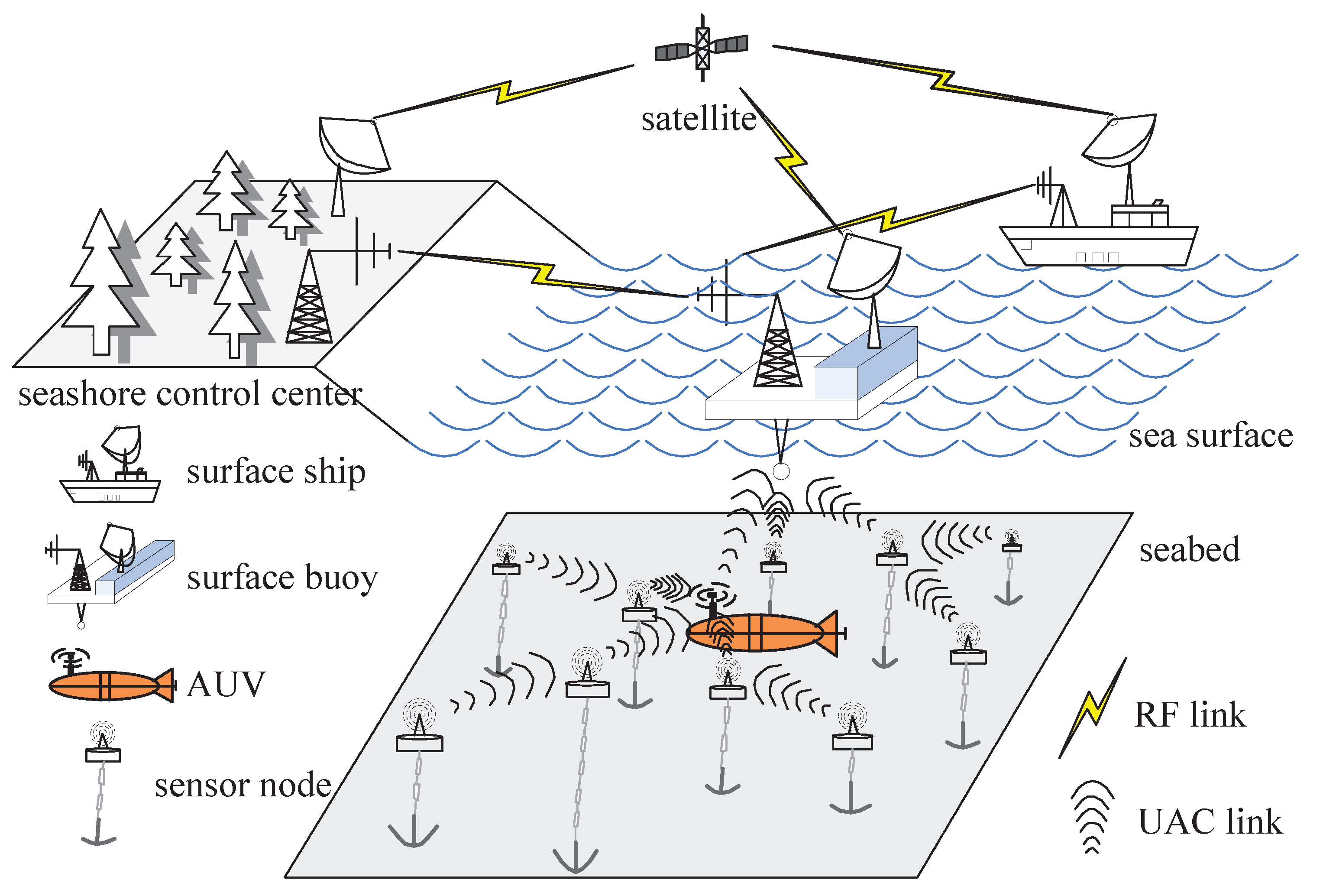
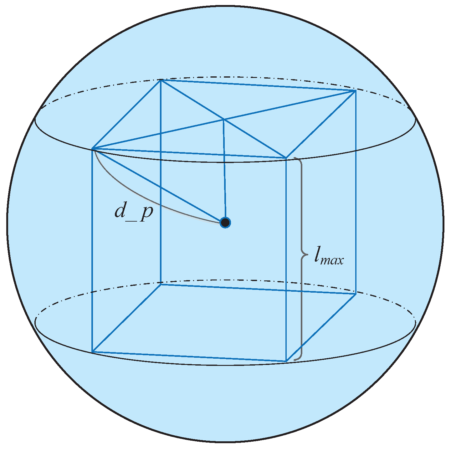
3.1. Network Model
3.2. Communication Model
4. Proposed Data Collection Algorithms
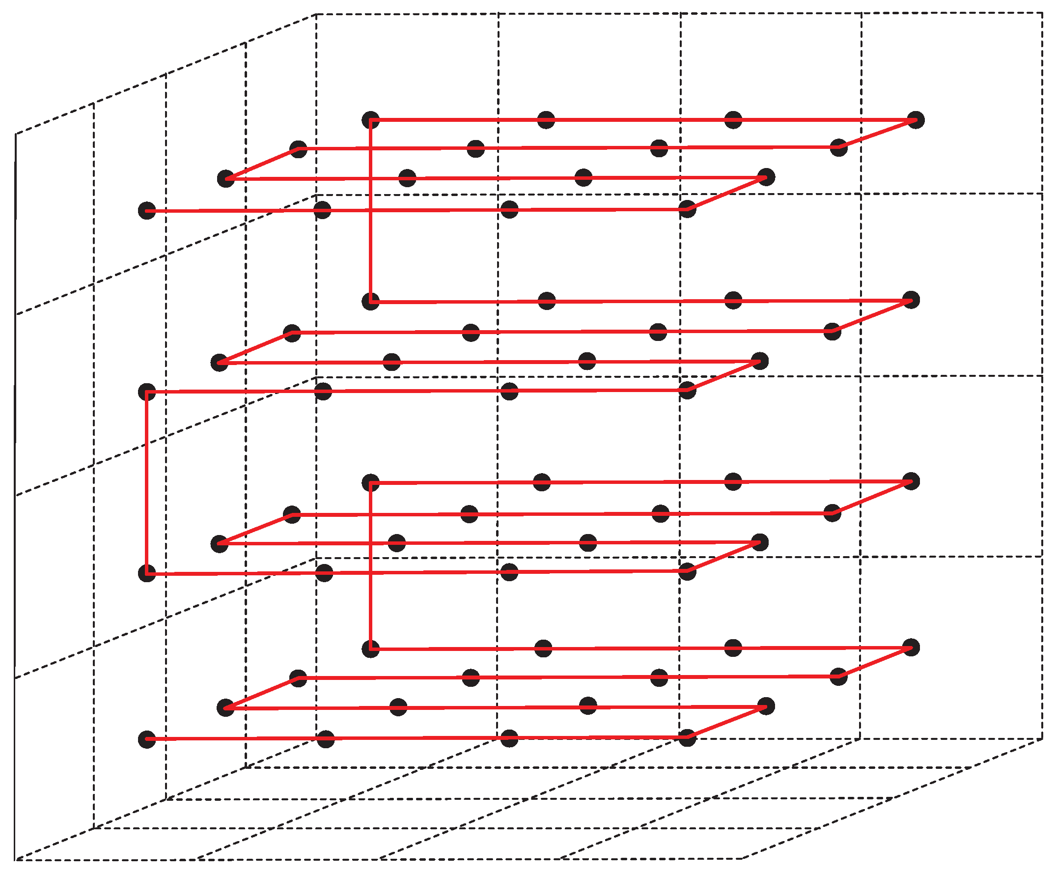
4.1. Grid and Probabilistic Neighborhood-Based Data Collection Algorithm with Layered-Scan(GPN-LSCAN)
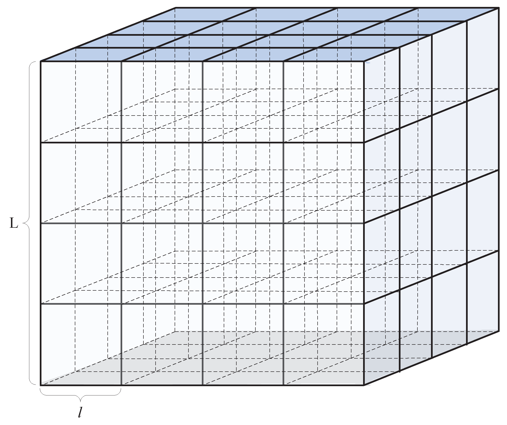
4.1.1. Network Partition Phase
4.1.2. AUV Trajectory Planning Phase
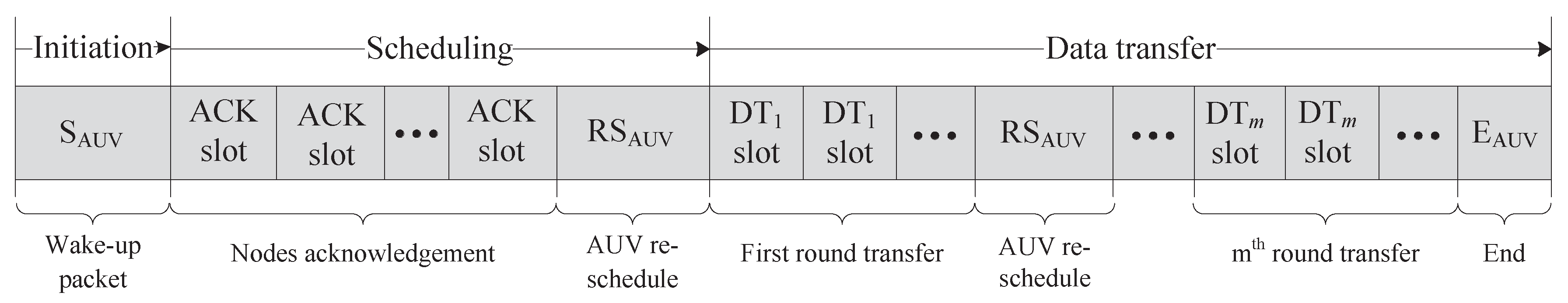
4.1.3. Data Collection Phase
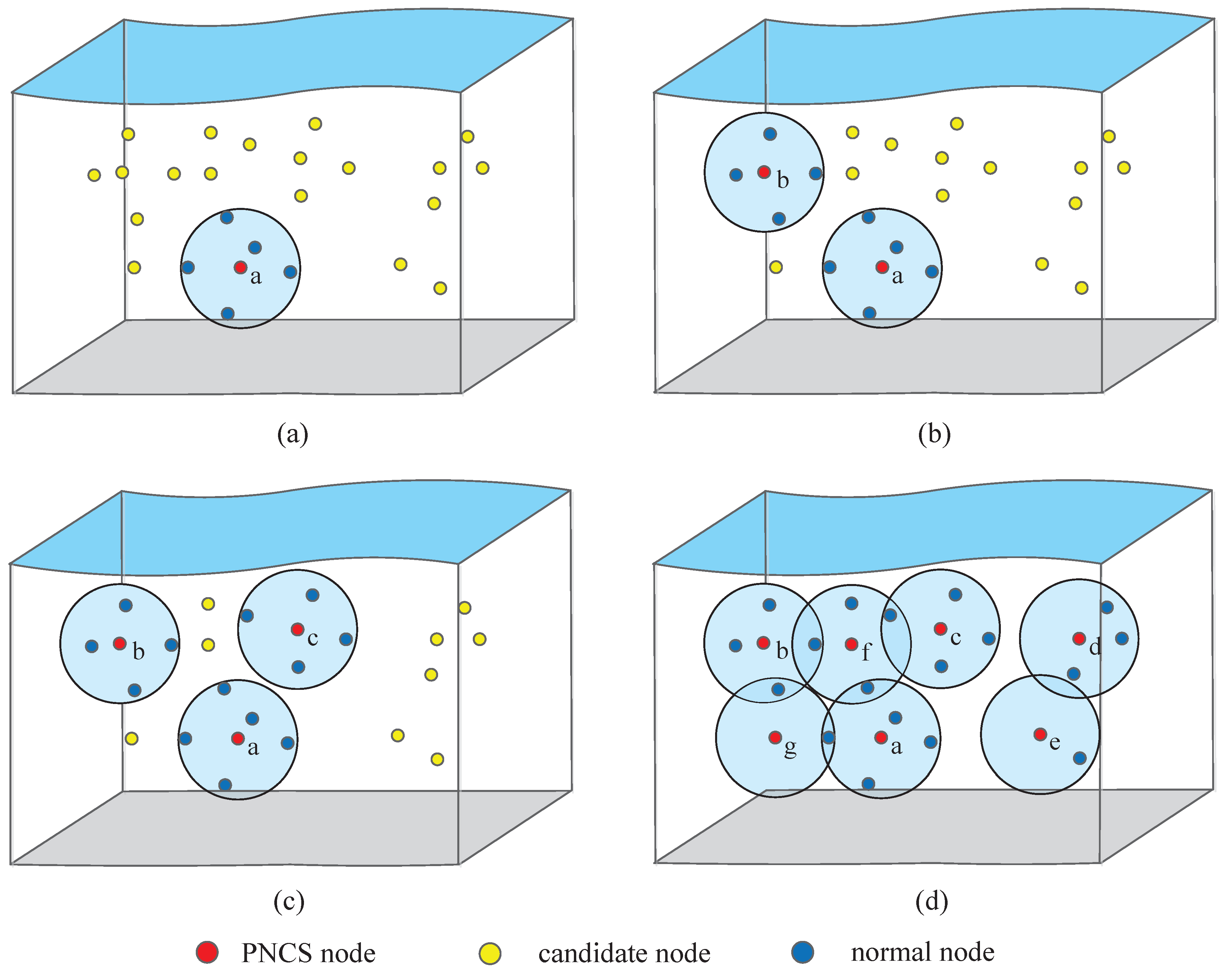
4.2. Probabilistic Neighborhood Covering Set-Based Greedy Heuristic Algorithm (PNCS-GHA)
4.2.1. Probabilistic Neighborhood Covering Set Construction Phase
| Algorithm 1 Probabilistic neighborhood covering set construction |
| Input: The candidate nodes set ; the locations of nodes in N; the parameter p; |
Output: The minimum probabilistic neighborhood covering set, S;
|
4.2.2. AUV Trajectory Planning Phase
| Algorithm 2 Planning the AUV trajectory in PNCS-GHA |
| Input: The constructed probabilistic neighborhood covering set S; the locations of nodes in S; |
Output: The traveling path of the AUV, P;
|
5. Performance Evaluation
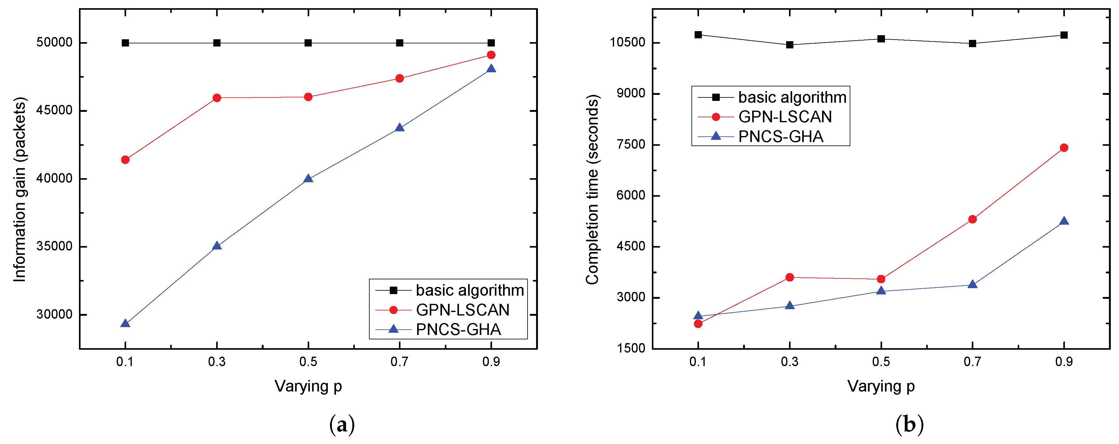
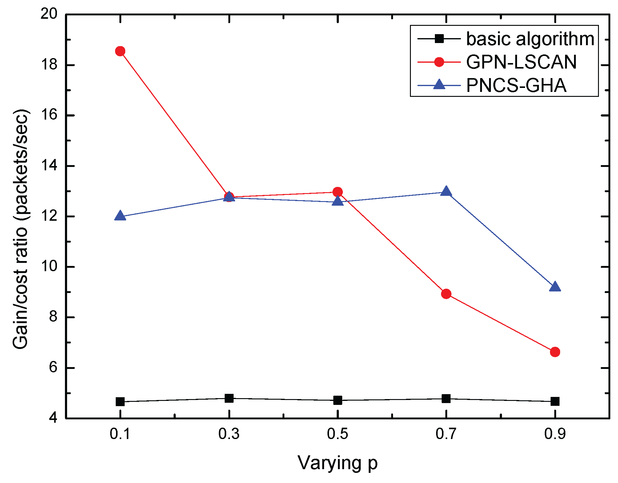
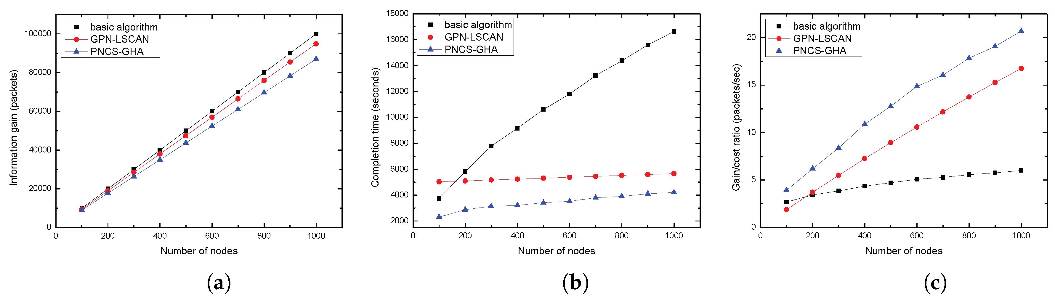
5.1. Data Collection Performance Comparison
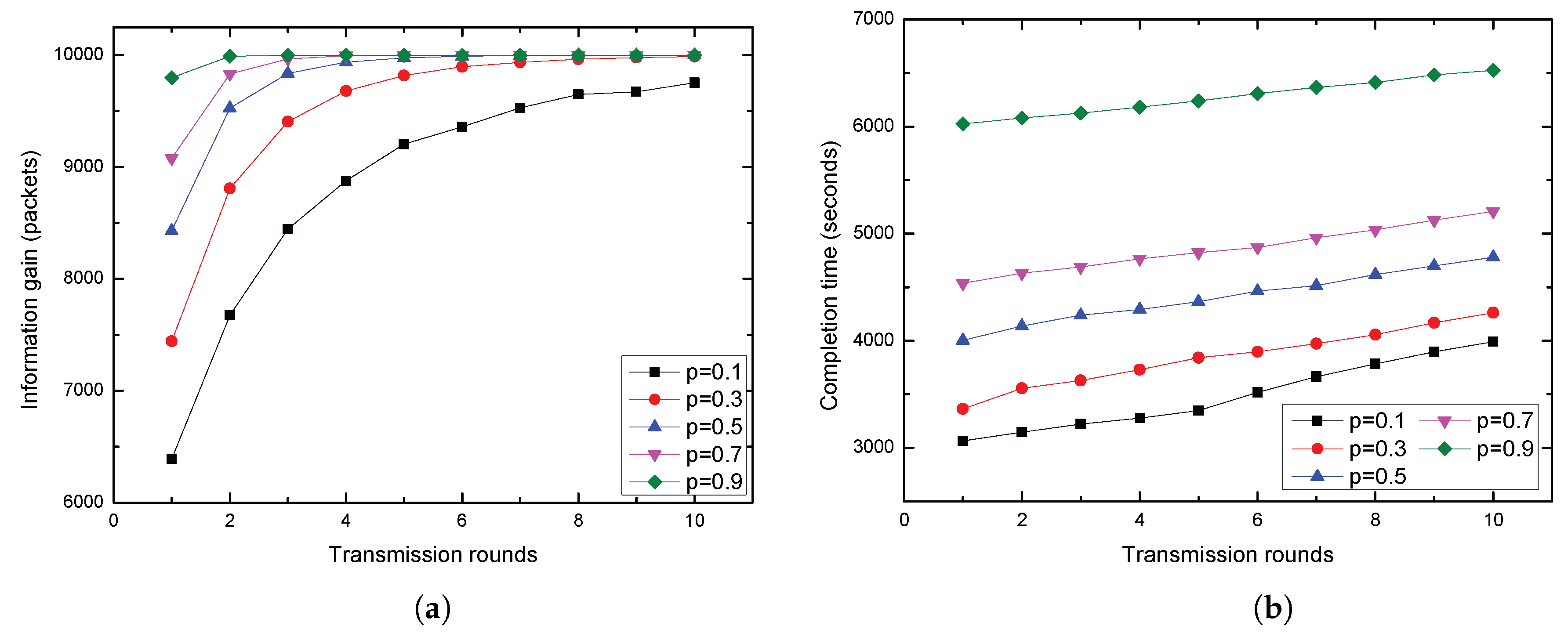
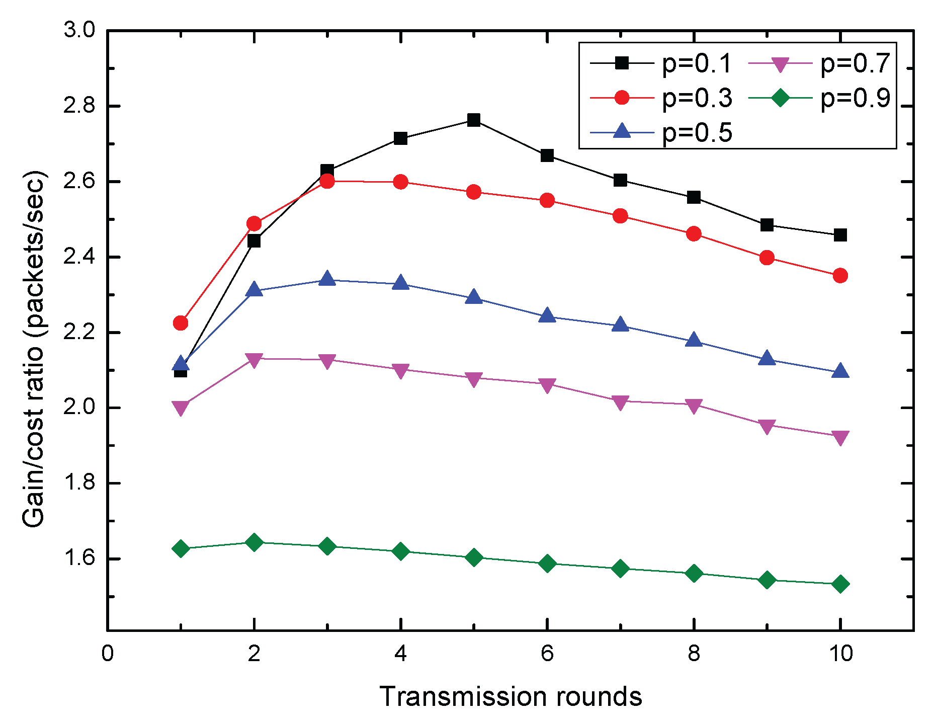
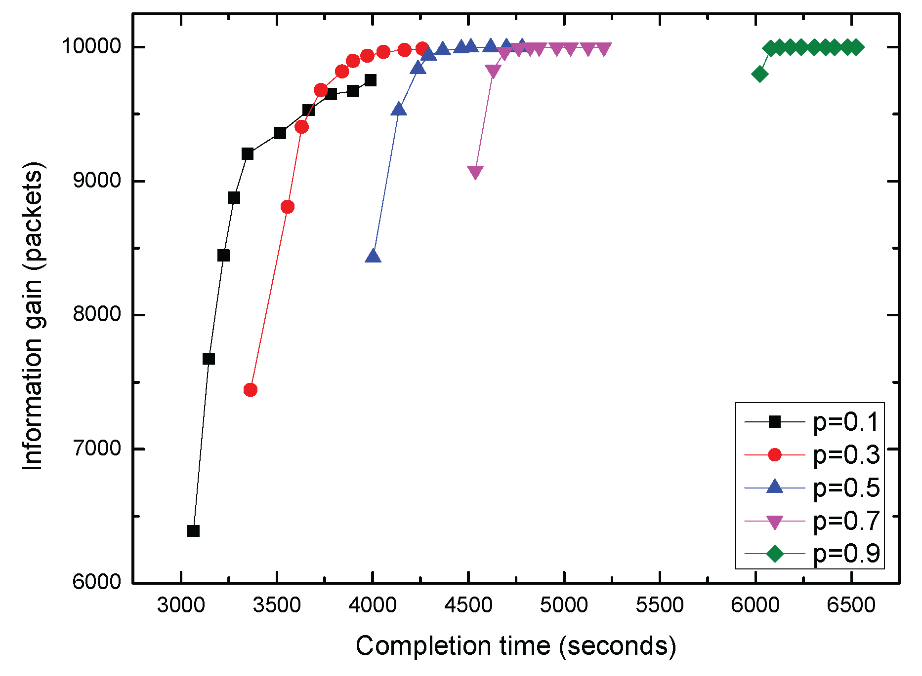
5.2. Performance Comparison for PNCS-GHA under Different Transmission Rounds
6. Conclusions
Acknowledgments
Author Contributions
Conflicts of Interest
References
- Zhu, C.; Leung, V.C.M.; Shu, L.; Ngai, E.C.H. Green Internet of Things for Smart World. IEEE Access 2015, 3, 2151–2162. [Google Scholar] [CrossRef]
- Qiu, T.; Chen, N.; Li, K.; Qiao, D.; Fu, Z. Heterogeneous Ad Hoc Networks: Architectures, Advances and Challenges. Ad Hoc Networks 2017, 55, 143–152. [Google Scholar] [CrossRef]
- Dong, C.; Zhou, J.; Wang, M. Application of the Internet of Things Technology in Smart Grid. Adv. Social Sci. Educ. Hum. Res. 2015, 39, 1022–1025. [Google Scholar]
- Chang, C.; Kuo, C.; Chen, J.; Wang, T. Design and Implementation of an IoT Access Point for Smart Home. Appl. Sci. 2015, 5, 1882–1903. [Google Scholar] [CrossRef]
- Liang, F.; Bai, H.; Liu, G. Application of Internet of Things in Military Equipment Logistics. Appl. Mech. Mater. 2014, 556–562, 6723–6726. [Google Scholar] [CrossRef]
- Ma, Y.; Zhang, Y.; Dung, O.M. Health Internet of Things: Recent Applications and Outlook. J. Internet Technol. 2015, 16, 351–362. [Google Scholar]
- Wu, D.; Dai, L.; Dai, H. Application of Internet of Thing Technology in Ecological-Environmental Protection of Long-Distance Water Diversion Project. Appl. Mech. Mater. 2015, 2563–2566. [Google Scholar] [CrossRef]
- Spalazzi, L.; Taccari, G.; Bernardini, A. An Internet of Things Ontology for Earthquake Emergency Evaluation and Response. In Proceedings of the International Conference on Collaboration Technologies and Systems, Minneapolis, MN, USA, 19–23 May 2014; pp. 528–534.
- Zhou, Z.; Yao, B.; Xing, R.; Shu, L.; Bu, S. E-CARP: An Energy Efficient Routing Protocol for UWSNs in the Internet of Underwater Things. IEEE Sens. J. 2016, 16, 4072–4082. [Google Scholar] [CrossRef]
- Han, G.; Jiang, J.; Sun, N.; Shu, L. Secure Communication for Underwater Acoustic Sensor Networks. IEEE Commun. Mag. 2015, 53, 54–60. [Google Scholar] [CrossRef]
- Han, G.; Jiang, J.; Shu, L.; Guizani, M. An Attack-Resistant Trust Model based on Multidimensional trust Metrics in Underwater Acoustic Sensor Networks. IEEE Trans. Mob. Comput. 2015, 14, 2447–2459. [Google Scholar] [CrossRef]
- Ayaz, M.; Baig, I.; Abdullah, A.; Faya, I. A Survery on Routing Techniques in Underwater Wireless Sensor Networks. Int. J. Comput. Appl. 2011, 34, 1908–1927. [Google Scholar]
- Han, G.; Jiang, J.; Bao, N.; Wan, L.; Guizani, M. Routing Protocols for Underwater Wireless Sensor Networks. IEEE Commun. Mag. 2015, 53, 72–78. [Google Scholar] [CrossRef]
- Kishigami, W.; Tanigawa, Y.; Tode, H. Robust Data Gathering Method Using Controlled Mobility in Underwater Sensor Network. In Proceedings of the IEEE International Conference on Sensing, Communication, and Networking (SECON), Singapore, 30 June–3 July 2014; pp. 176–178.
- Anupama, K.R.; Sasidharan, A.; Vadlamani, S. A Location-Based Clustering Algorithm for Data Gathering in 3D Underwater Wireless Sensor Networks. In Proceedings of the International Symposium on Telecommunications, Tehran, Iran, 27–28 August 2008; pp. 343–348.
- Domingo, M.C. A Distributed Energy-Aware Routing Protocol for Underwater Wireless Sensor Networks. Wirel. Pers. Commun. 2011, 57, 607–627. [Google Scholar] [CrossRef] [Green Version]
- Kartha, J.J.; Jabbar, A.; Baburaj, A.; Jacob, L. Maximum Lifetime Routing in Underwater Sensor Networks using Mobile Sink for Delay-Tolerant Applications. In Proceedings of the TENCON IEEE Region 10 Conference Proceedings, Macao, China, 1–4 November 2015; pp. 1–6.
- Kartha, J.J.; Jacob, L. Delay and Lifetime Performance of Underwater Wireless Sensor Networks with Mobile Element Based Data Collection. Int. J. Distrib. Sens. Netw. 2015, 2015, 1–22. [Google Scholar]
- Ilyas, N.; Alghamdi, T.A.; Farooq, M.N. AEDG: AUV-aided Efficient Data Gathering Routing Protocol for Underwater Wireless Sensor Networks. Procedia Comput. Sci. 2015, 52, 568–575. [Google Scholar] [CrossRef]
- Hollinger, G.A.; Choudhary, S.; Qarabaqi, P.; Murphy, C.; Mithra, U.; Sukhatme, G.S.; Stojanovic, M.; Singh, H.; Hover, F. Underwater Data Collection using Robotic Sensor Networks. IEEE J. Sel. Areas Commun. 2012, 30, 899–911. [Google Scholar] [CrossRef]
- Hollinger, G.A.; Mitra, U.; Sukhatme, G. Autonomous Data Collection from Underwater Sensor Networks using Acoustic Communication. In Proceedings of the IEEE International Conference on Intelligent Robots and Systems, Francisco, CA, USA, 25–30 September 2011; pp. 3564–3570.
- Han, G.; Liu, L.; Jiang, J.; Shu, L.; Rodrigues, J.J.P.C. A Collaborative Secure Localization Algorithm Based on Trust Model in Underwater Wireless Sensor Networks. Sensors 2016, 16, 229. [Google Scholar] [CrossRef] [PubMed]
- Han, G.; Jiang, J.; Zhang, C.; Duong, T.Q.; Guizani, M.; Karagiannidis, G. A Survey on Mobile Anchors Assisted Localization in Wireless Sensor Networks. IEEE Commun. Surv. Tutorials 2016, 18, 2220–2243. [Google Scholar] [CrossRef]
- Han, G.; Zhang, C.; Shu, L.; Rodrigues, J.J.P.C. Impacts of Deployment Strategies on Localization Performances in Underwater Acoustic Sensor Networks. IEEE Trans. Ind. Electron. 2015, 62, 1725–1733. [Google Scholar] [CrossRef]
- Hollinger, G.A.; Yerramalli, S.; Singh, S.; Mitra, U.; Sukhatme, G.S. Distributed Coordination and Data Fusion for Underwater Search. In Proceedings of the IEEE International Conference on Robotics and Automation, Shanghai, China, 9–13 May 2011; pp. 349–355.
- Arrichiello, F.; Liu, D.N.; Yerramalli, S.; Pereira, A.; Das, J.; Mitra, U.; Sukhatme, G.S. Effects of Underwater Communication Constraints on the Control of Marine Robot Teams. In Proceedings of the International Conference on Robot Communication and Coordination, Odense, Denmark, 31 March–2 April 2009; pp. 1–8.
- Stojanovic, M. On the Relationship between Capacity and Distance in an Underwater Acoustic Communication Channel. In Proceedings of the First ACM International Workshop on Underwater Networks, Los Angeles, CA, USA, 25 September 2006; pp. 41–47.
- Berkhovskikh, L.; Lysanov, Y. Fundamentals of Ocean Acoustics; Springer: New York, NY, USA, 1982. [Google Scholar]
- Cui, H.; Wang, Y.; Lv, J. Path Planning of Mobile Anchor in Three-dimensional Wireless Sensor Networks for Localization. J. Inf. Comput. Sci. 2012, 9, 2203–2210. [Google Scholar]
- Gong, W.; Li, M. Comparison of Heuristics for Resolving the Traveling Salesman Problem with Information Technology. Adv. Mater. Res. 2014, 886, 593–597. [Google Scholar] [CrossRef]


| Parameters | Value |
|---|---|
| Network Size | 1000 × 1000 × 1000 m3 |
| Number of Nodes | 100–1000 |
| Parameter p | 0.9, 0.7, 0.5, 0.3, 0.1 |
| Probabilistic Neighborhood Contour | 150, 210, 240, 270, 300 (m) |
| Moving Speed of AUV | 2.5, 5 (m/s) |
| Transmission Frequency | 10 kHz |
| Transmission Power | 1 W |
| Transmission Round | 1–10 |
| Bandwidth | 4 kHz |
| Number of Each Node’s Data Packets | 100 packets |
© 2017 by the authors. Licensee MDPI, Basel, Switzerland. This article is an open access article distributed under the terms and conditions of the Creative Commons Attribution (CC BY) license ( http://creativecommons.org/licenses/by/4.0/).
Share and Cite
Han, G.; Li, S.; Zhu, C.; Jiang, J.; Zhang, W. Probabilistic Neighborhood-Based Data Collection Algorithms for 3D Underwater Acoustic Sensor Networks. Sensors 2017, 17, 316. https://doi.org/10.3390/s17020316
Han G, Li S, Zhu C, Jiang J, Zhang W. Probabilistic Neighborhood-Based Data Collection Algorithms for 3D Underwater Acoustic Sensor Networks. Sensors. 2017; 17(2):316. https://doi.org/10.3390/s17020316
Chicago/Turabian StyleHan, Guangjie, Shanshan Li, Chunsheng Zhu, Jinfang Jiang, and Wenbo Zhang. 2017. "Probabilistic Neighborhood-Based Data Collection Algorithms for 3D Underwater Acoustic Sensor Networks" Sensors 17, no. 2: 316. https://doi.org/10.3390/s17020316