
Lightdrum—Portable Light Stage for Accurate BTF Measurement on Site


Abstract
:1. Introduction
- a novel design and construction of a working prototype of a portable BTF/BRDF measuring device that allows for its positioning against a sample by means of an auto-collimator, thus permitting on site measurement in real life scenarios with high speed and accuracy,
- the first portable device for on site measurements where a viewing direction (two degrees of freedom) to the measured sample can be set continuously and arbitrarily for up to maximum zenith angle 75,
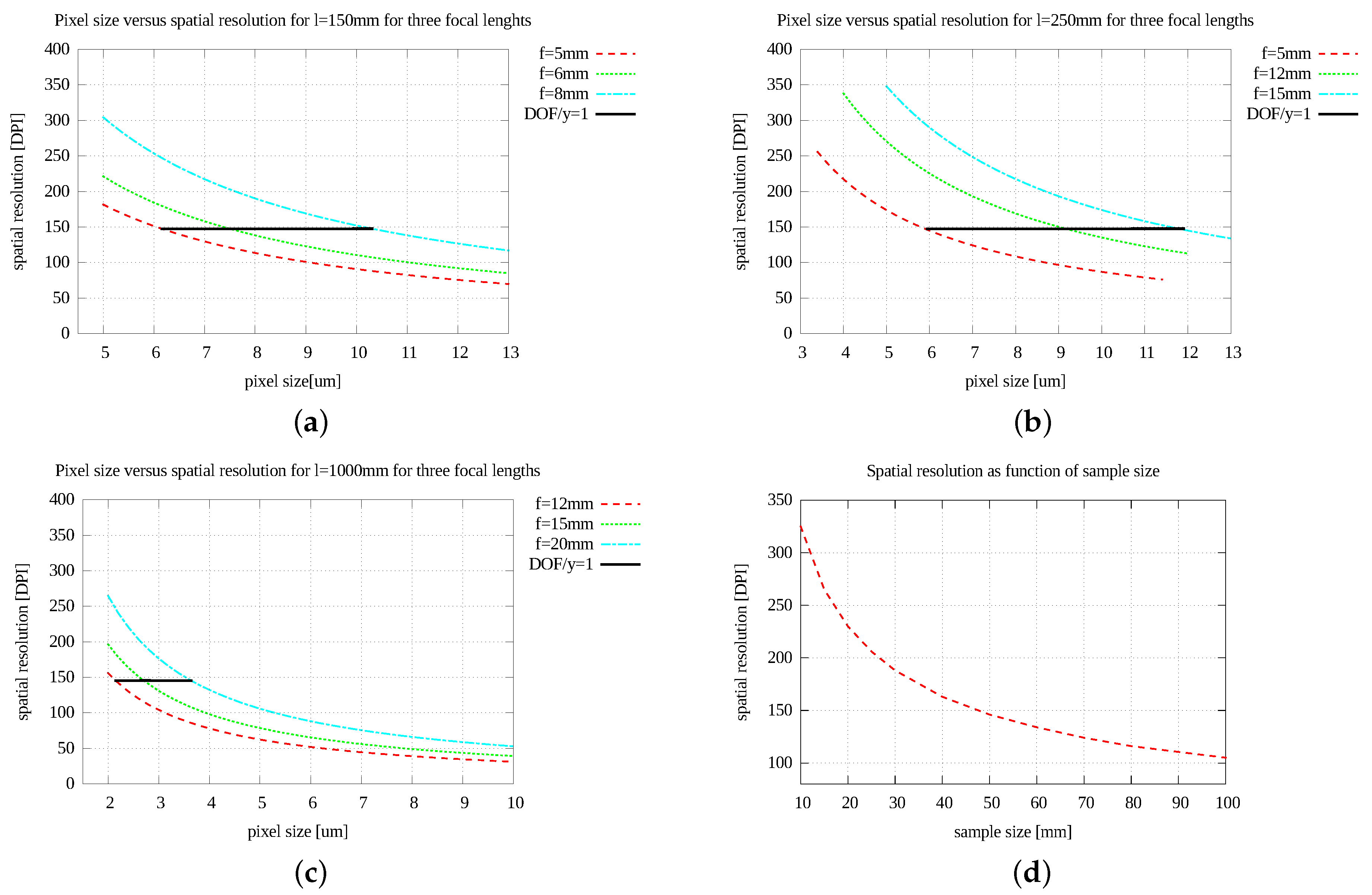
- a description of optical phenomena that limit either the spatial resolution or the size of the sample measured with BTF gantry,
- a marker sticker method for BTF/BRDF data acquisition which is used later in the data processing to align the data measured from the various camera directions,
- the documentation of our device construction by photographs of the individual parts and a step-by-step photographic documentation of the prototype assembly.
2. Related Work
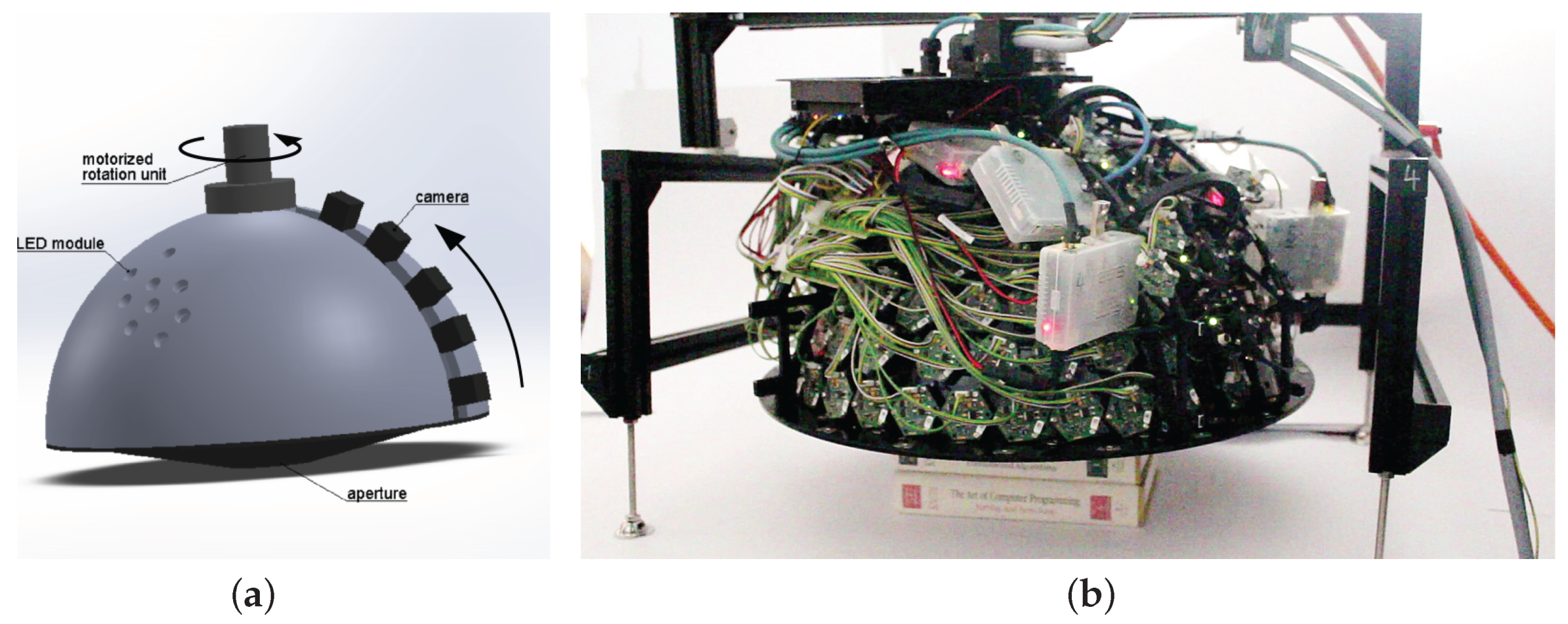
3. Lightdrum Overview
4. Mechanical Design
5. Cameras
5.1. Camera Selection and Optical Design
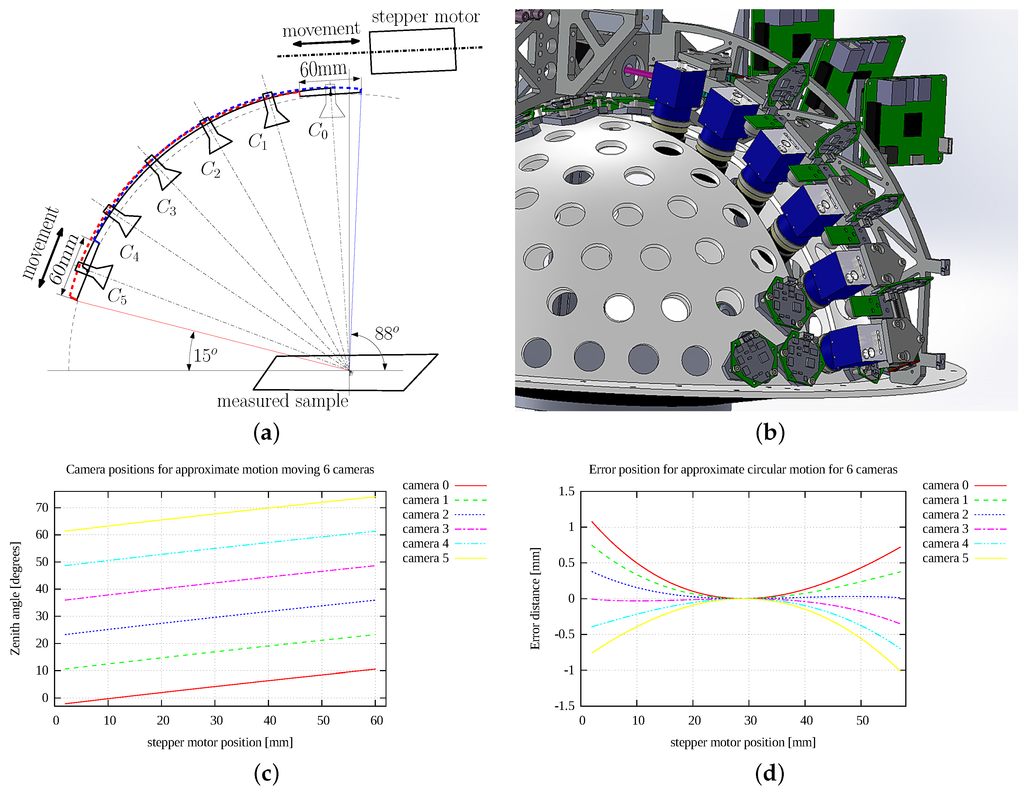
5.2. Camera Positioning
6. Illumination Units
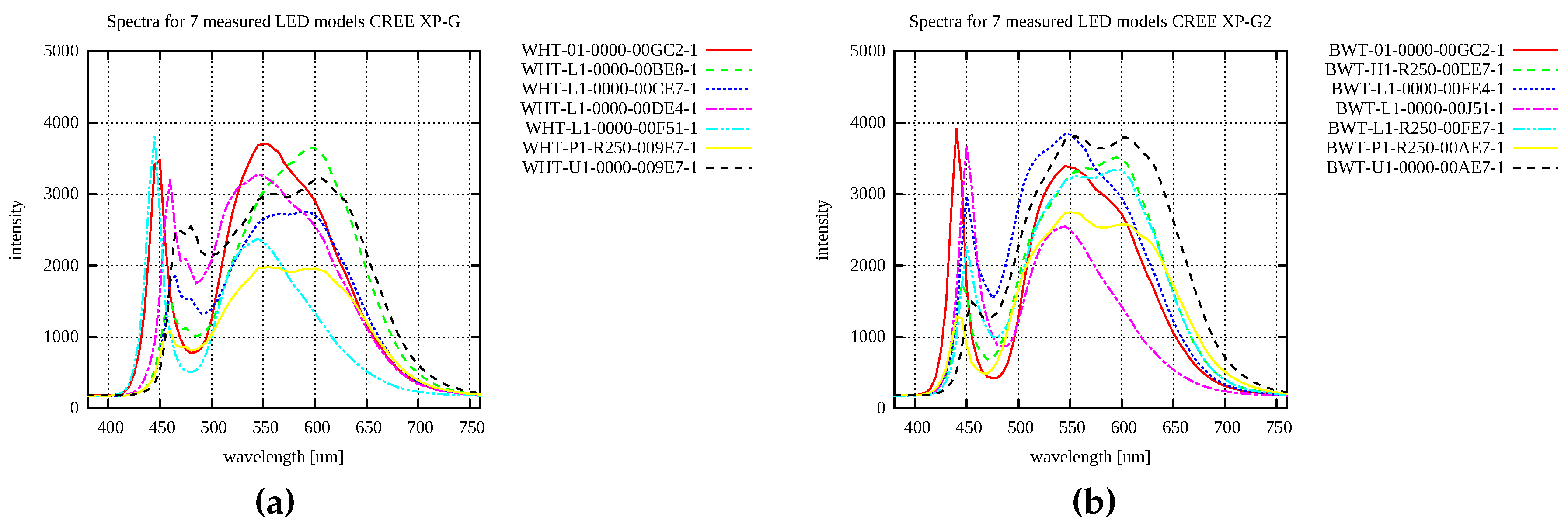
6.1. LED Selection
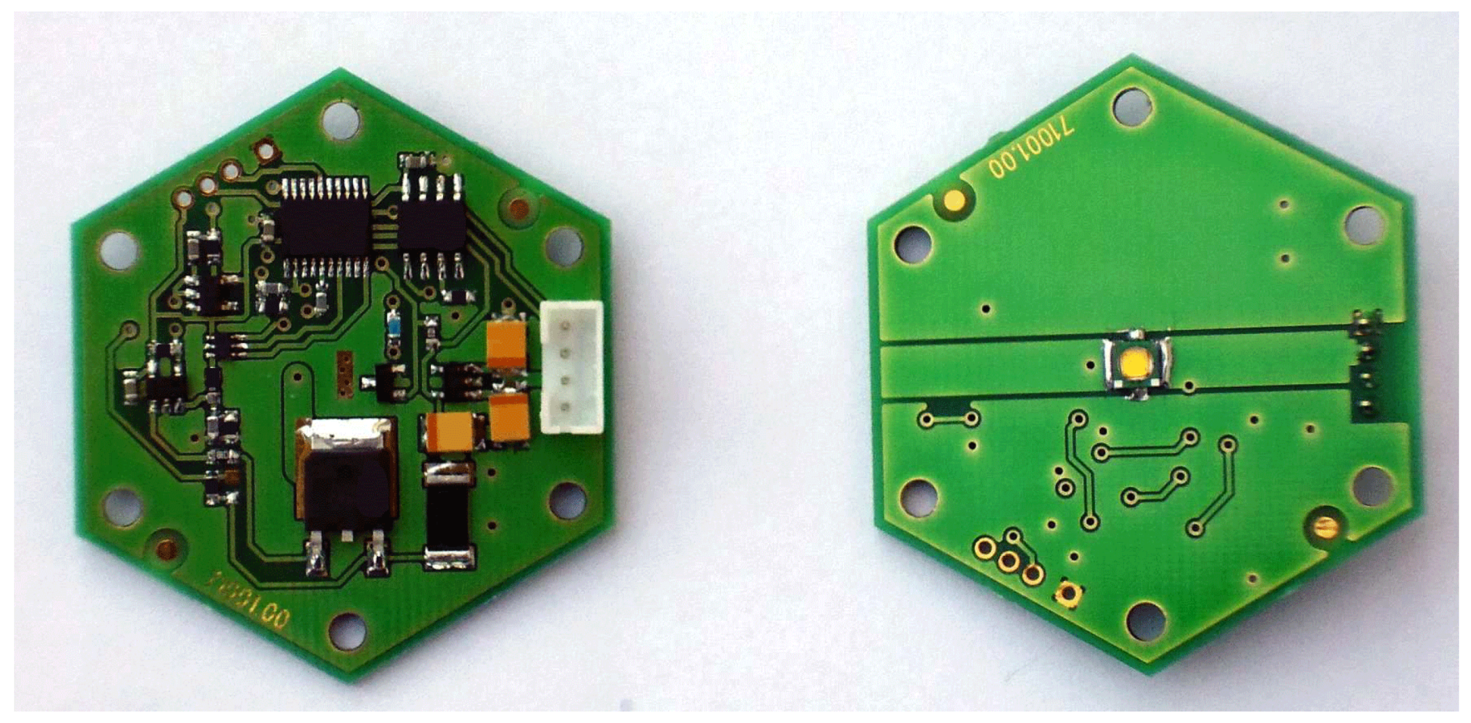
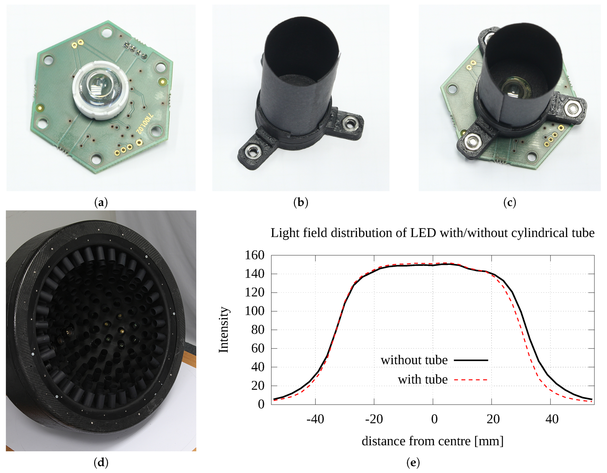
6.2. LED Modules
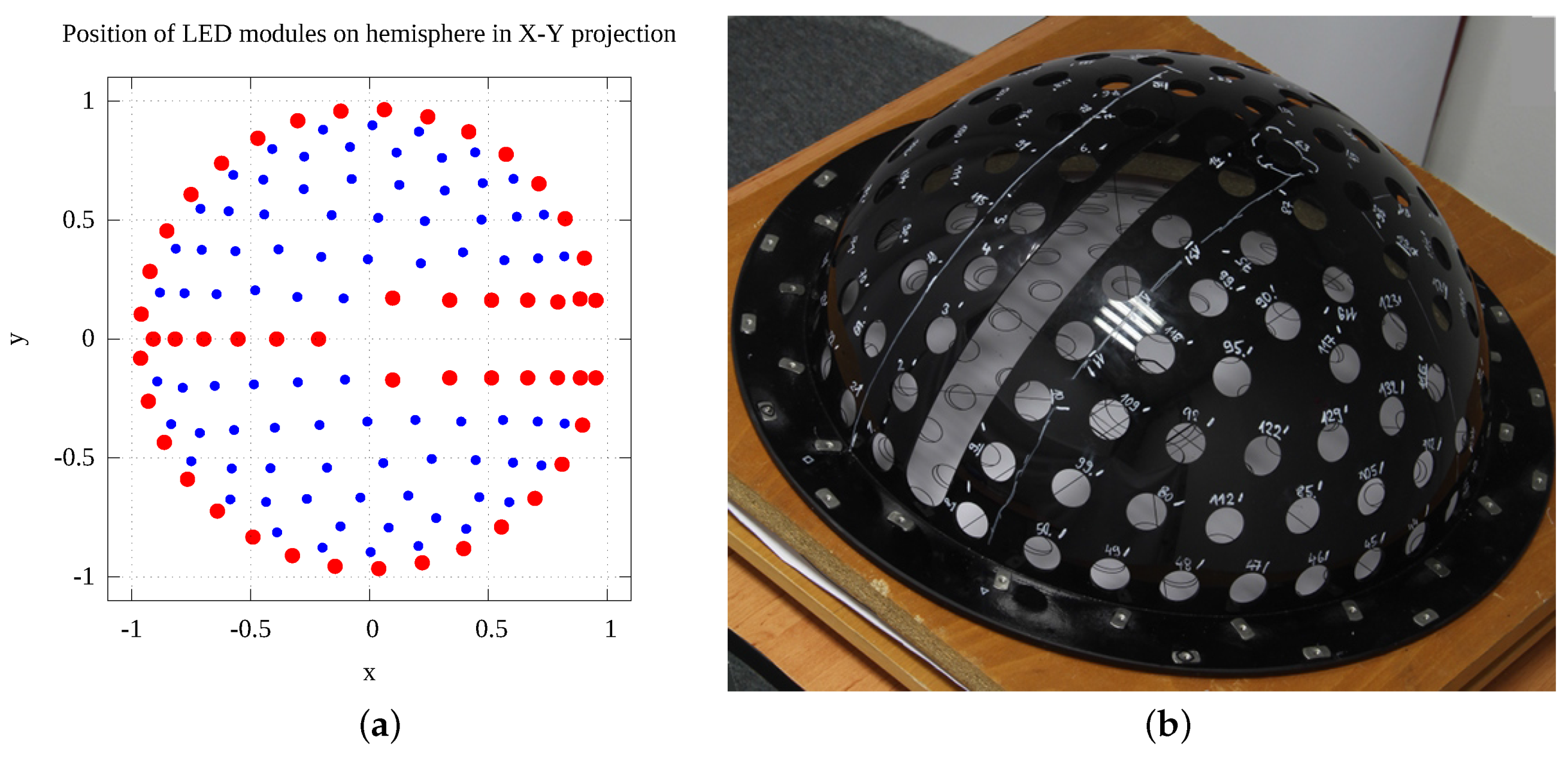
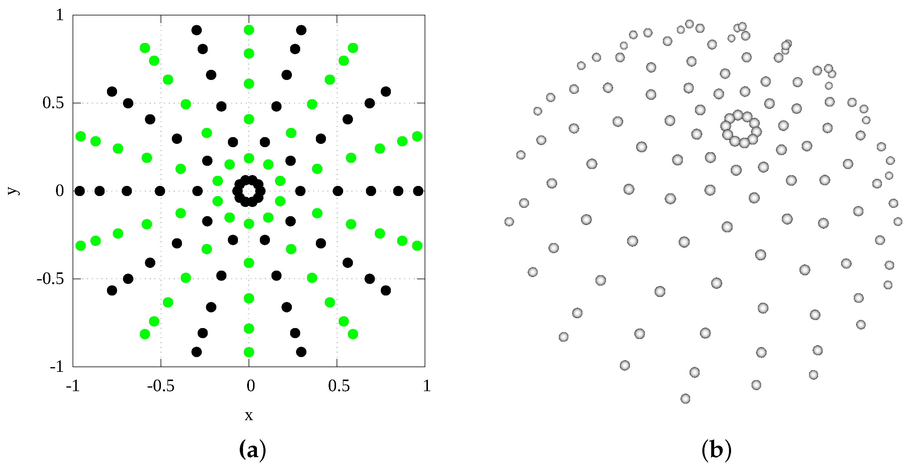
6.3. LED Modules Distribution on Hemispherical Dome
7. Other Measurement Issues
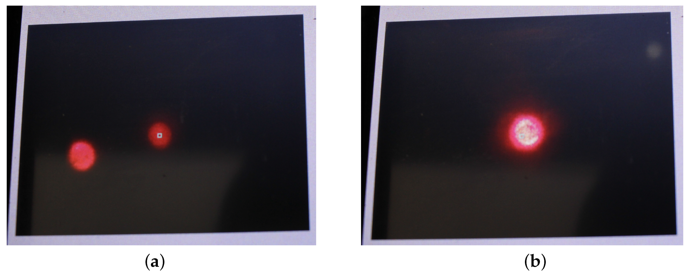
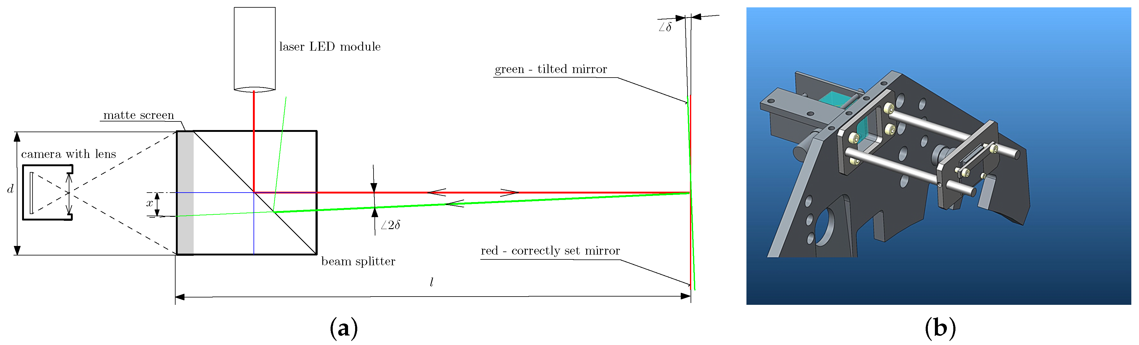
7.1. Auto-Collimator
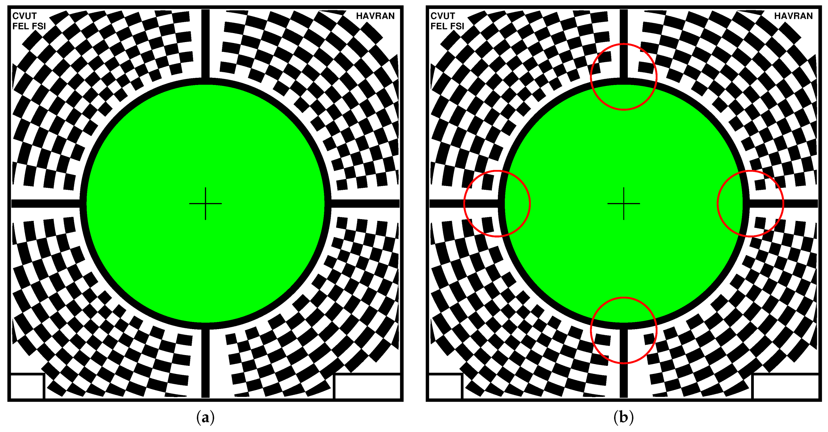
7.2. Marker Sticker Image Registration Method
7.3. Measurement Setup Procedure
- find a locally flat and appropriate position on the measured surface sample, verify it is accessible by the gantry,
- glue on the marker sticker with a selected orientation that can relate to the structure of the measured surface sample,
- temporarily fasten the mirror (by appropriate means such as power tape) so that the middle of the marker sticker contains the mirror, while the fastener of the mirror can be removed, and the border of the marker sticker with its centring marks is still visible. The 40 mm mirror width allows us to put the mirror at an angle of 45 to the centring marks so that they remain visible.
- position the measurement instrument, adjust both its perpendicularity and position against the sample using the mirror and centring marks on the marker sticker,
- carefully remove the mirror fasteners, and slide the mirror away from the instrument’s measurement aperture. The 500 mm length of the mirror allows for easy manipulation of the mirror upon its removal, before the measurement takes place.
- recheck the position of the instrument against the sample and start the measurement.
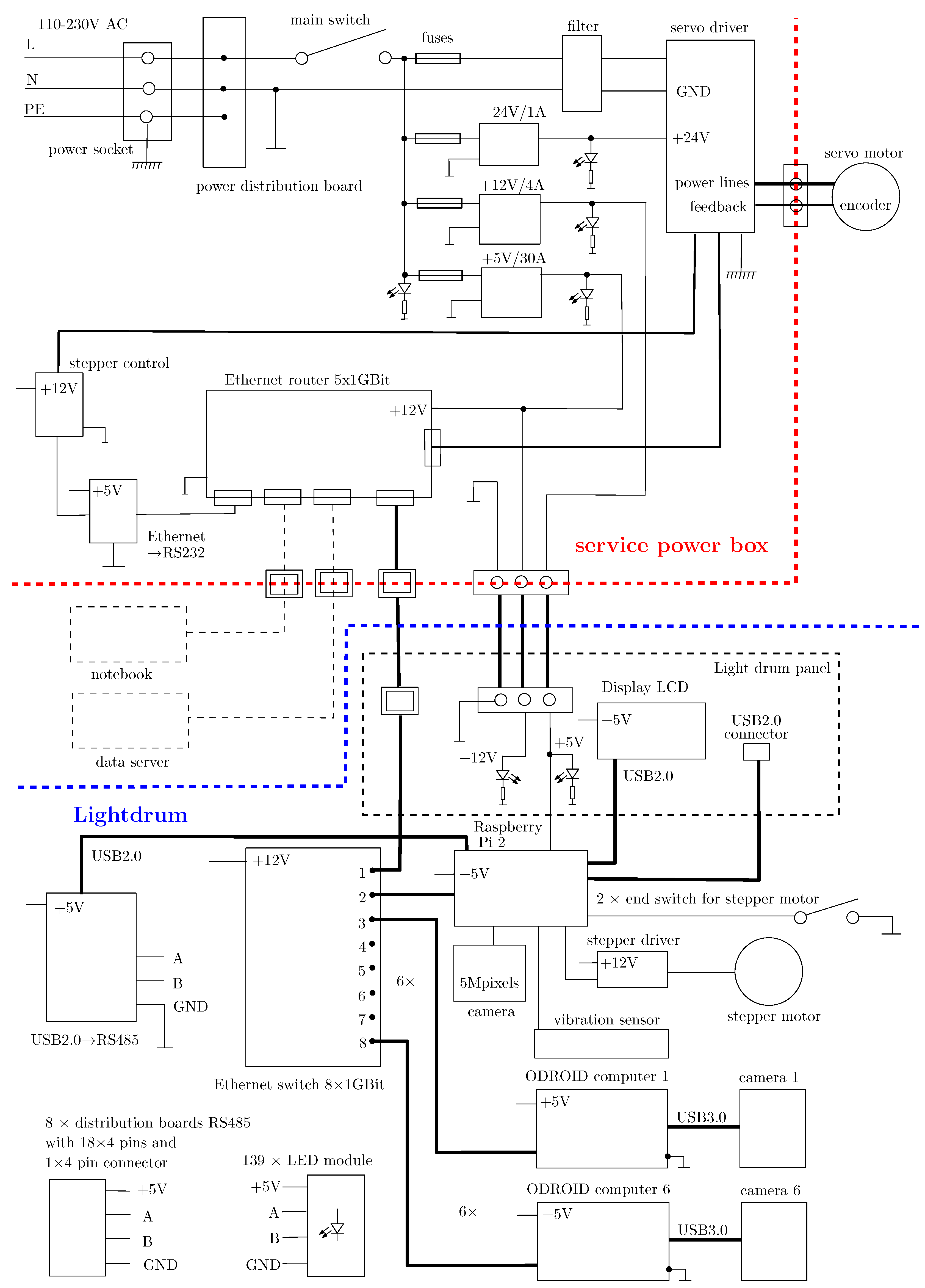
7.4. Electronics
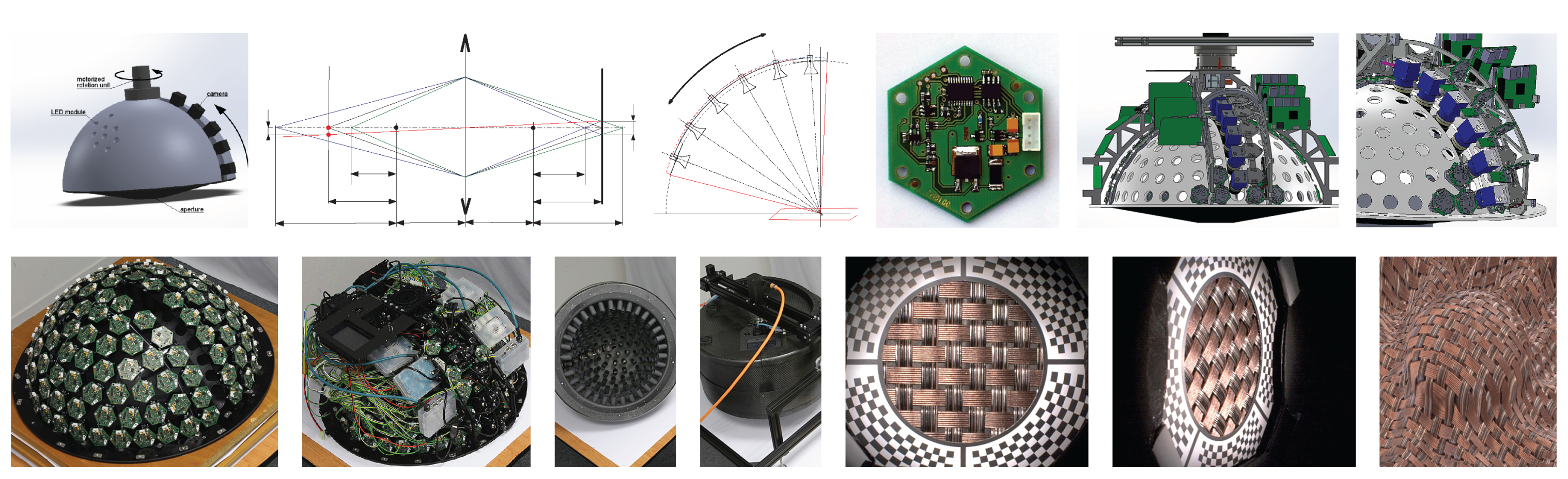
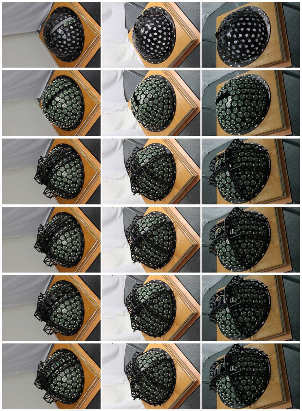
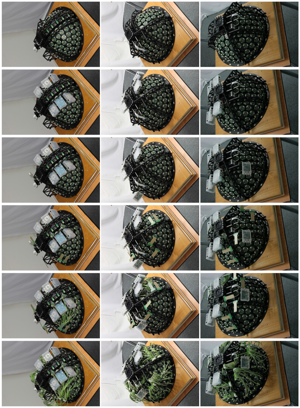
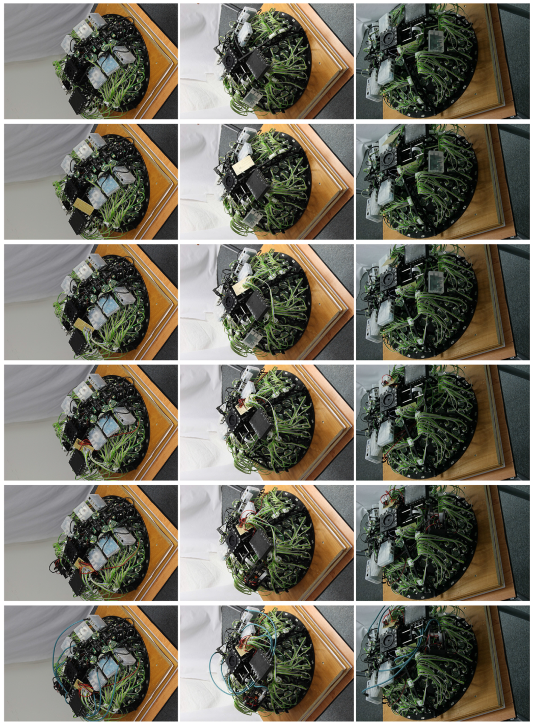
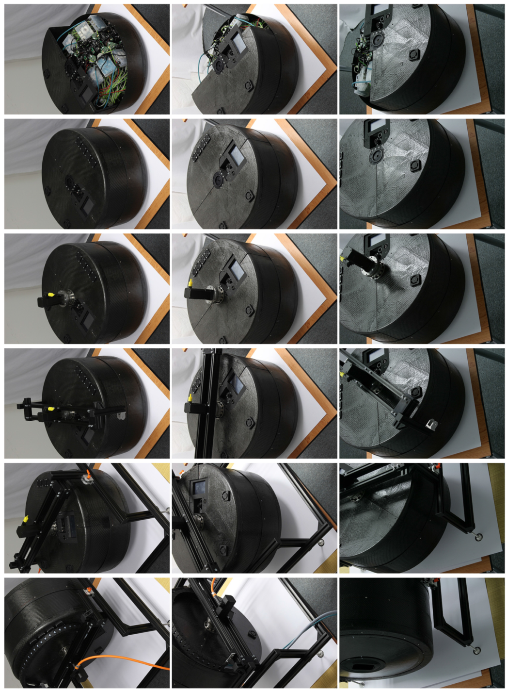
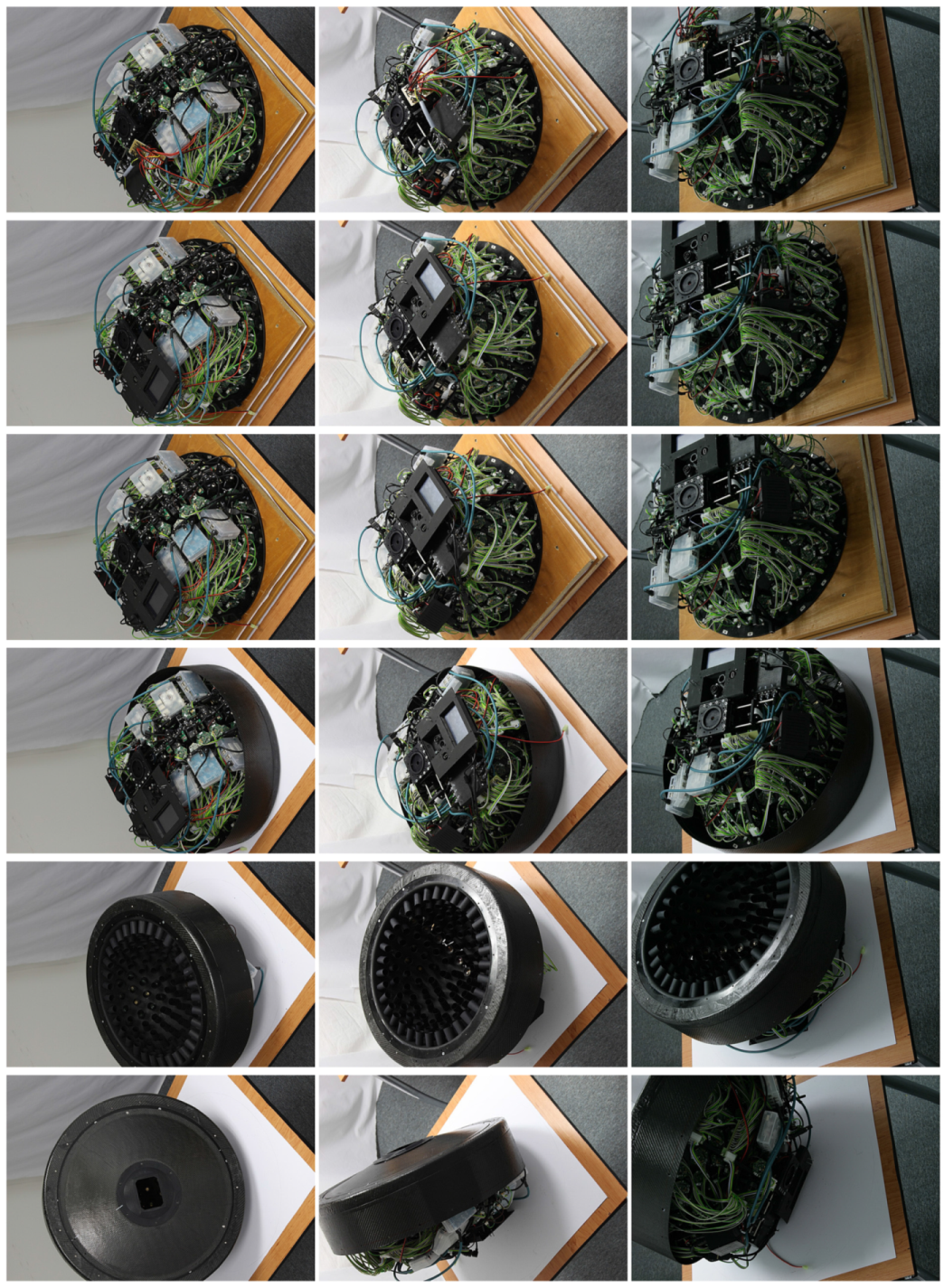
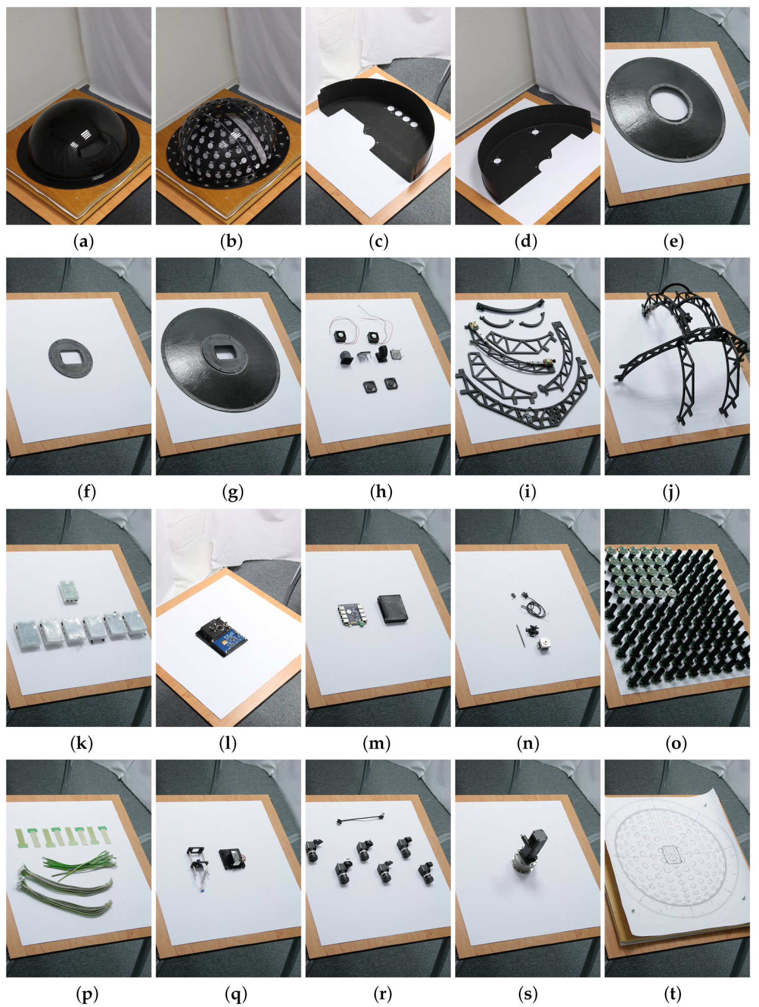
8. Parts Production, Assembly and Debugging
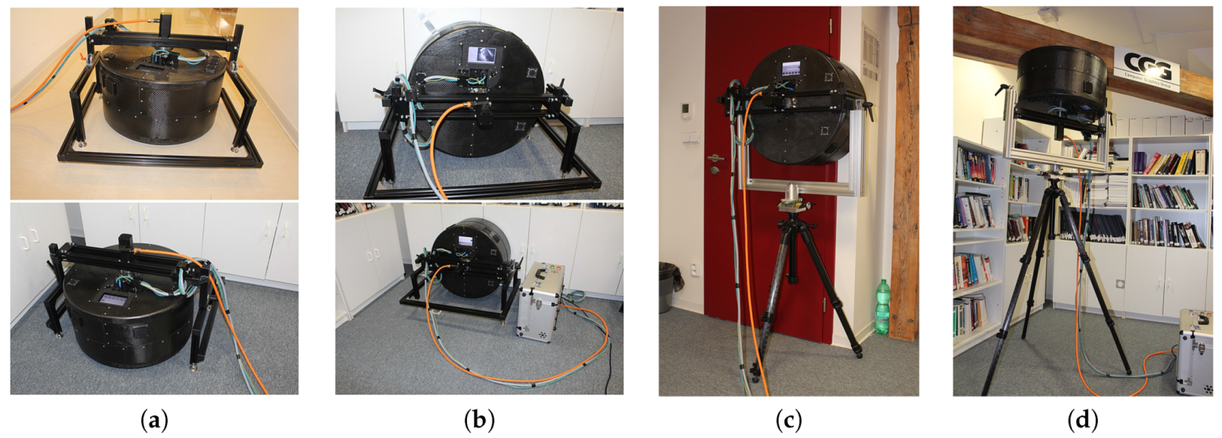
- the holding frame for measurement on the floor or the desk, or the tripod for measurement on the wall or ceiling, shown in Figure 4,
- the aluminium frame with geared servo motor (shown in Figure 16s) on which the lightdrum is mounted,
- the service power box with electronics (power supplies, servo motor drive, and gigabit Ethernet router), shown in Figure 4b,
- the outer carbon cover consisting of three parts, protecting the instrument from damage and disturbing external light, in Figure 16c–g,
- the inner aluminium frame construction that provides mechanical support and is mounted on the servo motor gear output, in Figure 16i,j,
- the PMMA dome mounted on the inner aluminium frame, in Figure 16a,b,
- the six cameras mounted on the approximate circular motion mechanism, in Figure 16r,
- the six embedded microcomputers for operating the cameras (Hardkernel Odroid-XU3), in Figure 16k,
- the additional 5 Mpixel camera connected to the Raspberry Pi 2 and the laser module for the auto-collimator, in Figure 16q,
- the embedded gigabit Ethernet switch and its cover, in Figure 16m,
- the 139 LED modules (in Figure 16o) mounted on the PMMA dome,
- the cables inside the lightdrum; power, RS485 (in Figure 16p), and gigabit Ethernet),
- and the three cables between the external service power box and the lightdrum with the servo motor, shown in Figure 4.
9. Adjustment
10. Data Acquisition and Calibration
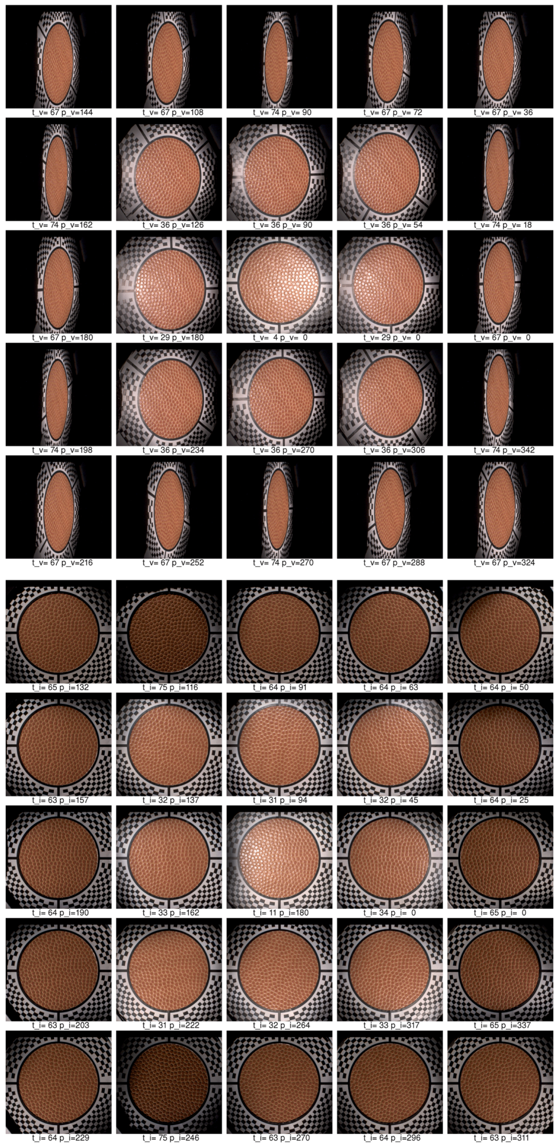
10.1. Data Acquisition
10.2. Radiometric and Colourimetric Calibration
11. Data Processing
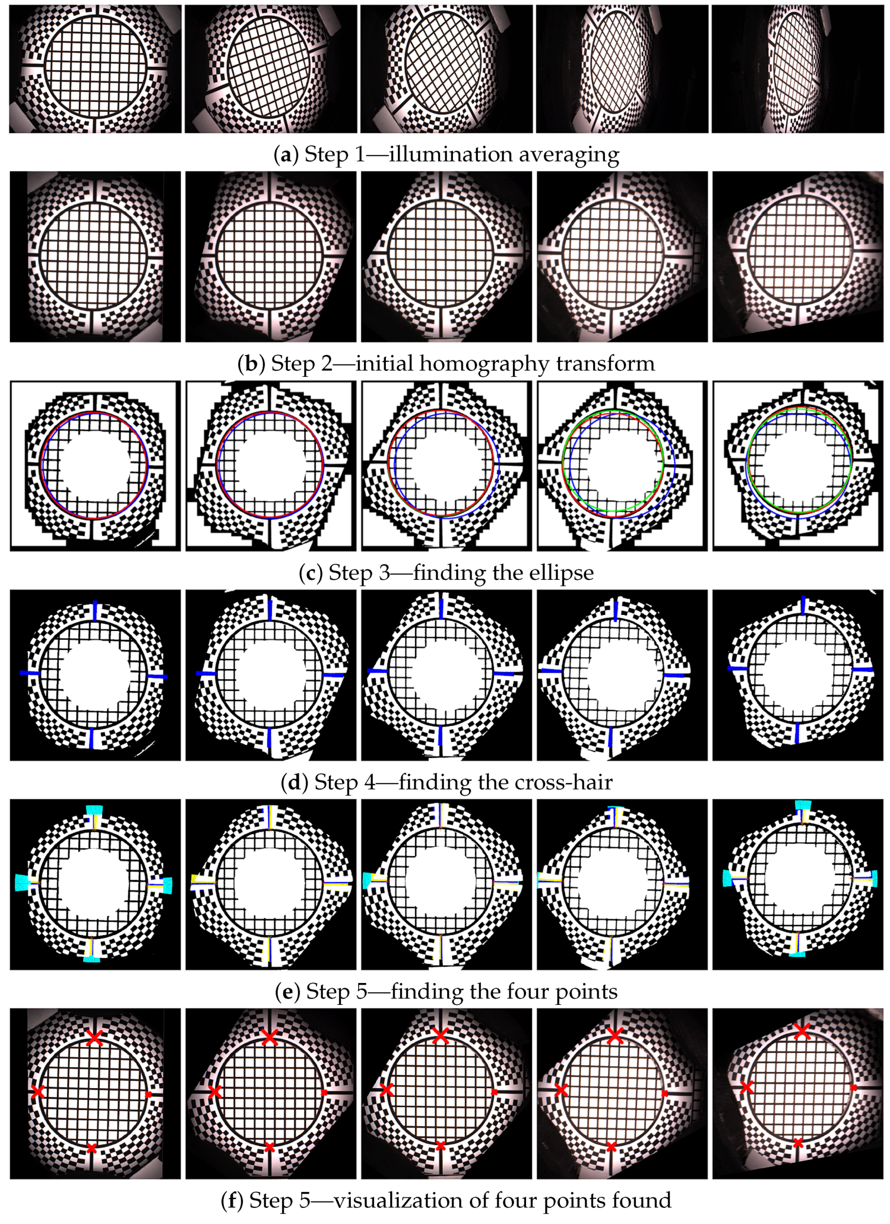
11.1. Step 1—Illumination Averaging
11.2. Step 2—Initial Homography Transform
11.3. Step 3—Ellipse Finding
11.4. Step 4—Cross-Hair Finding
11.5. Step 5—Four Points Location
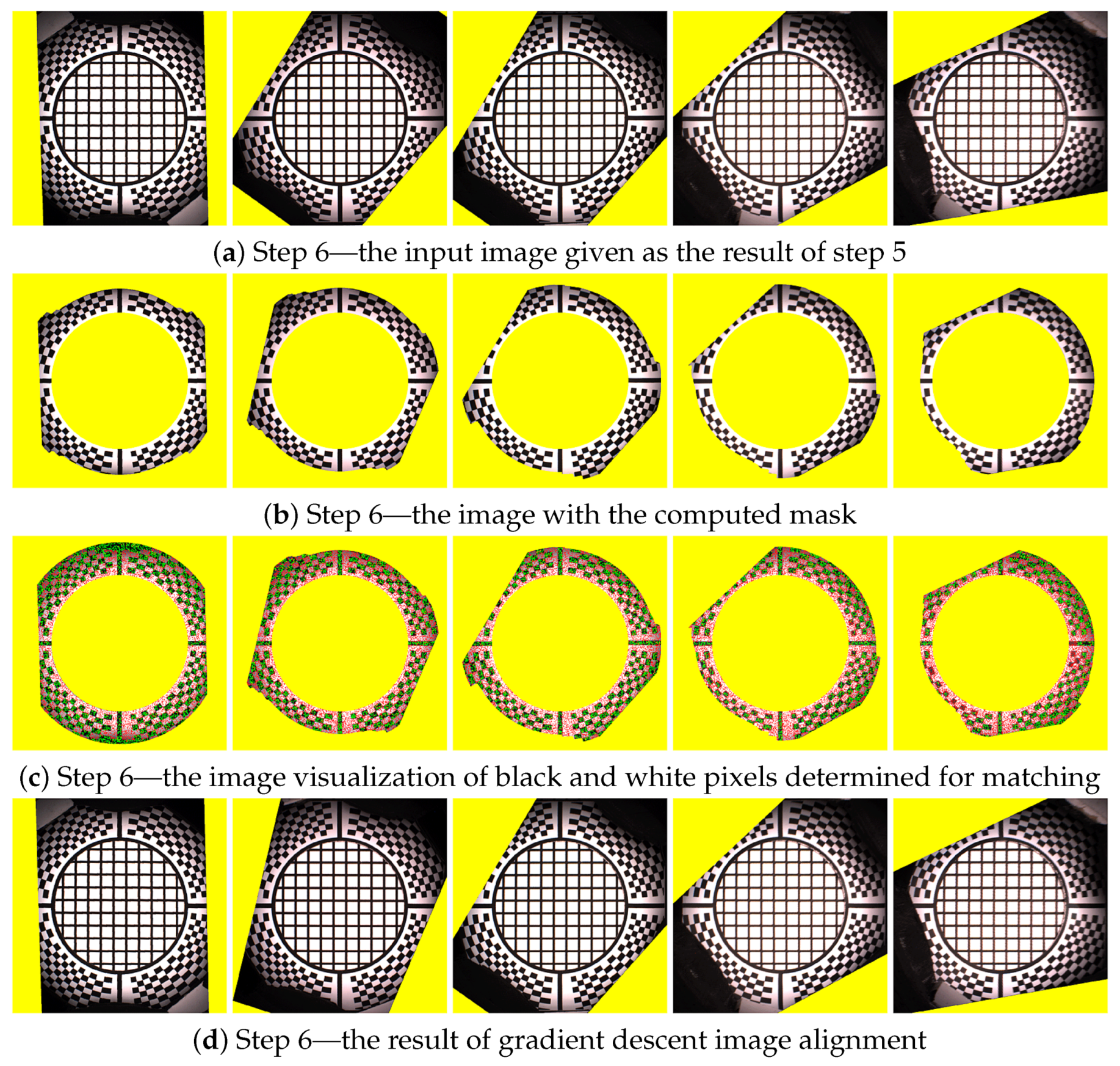
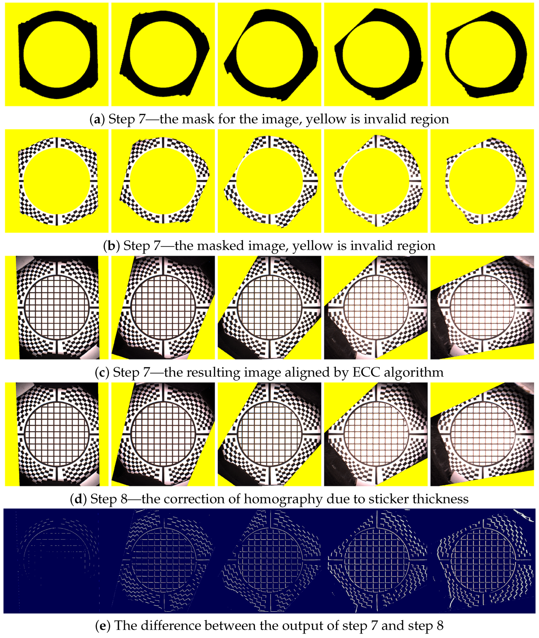
11.6. Step 6—Chequerboard Fitting
11.7. Step 7—Chequerboard Subpixel Fitting
11.8. Step 8—Marker Sticker Thickness Correction
11.9. Step 9—Data Transform and Processing
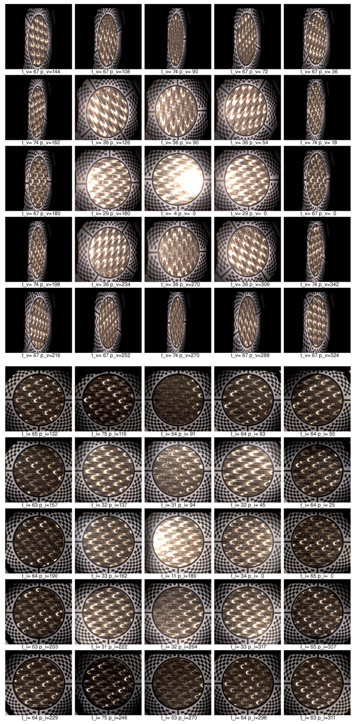
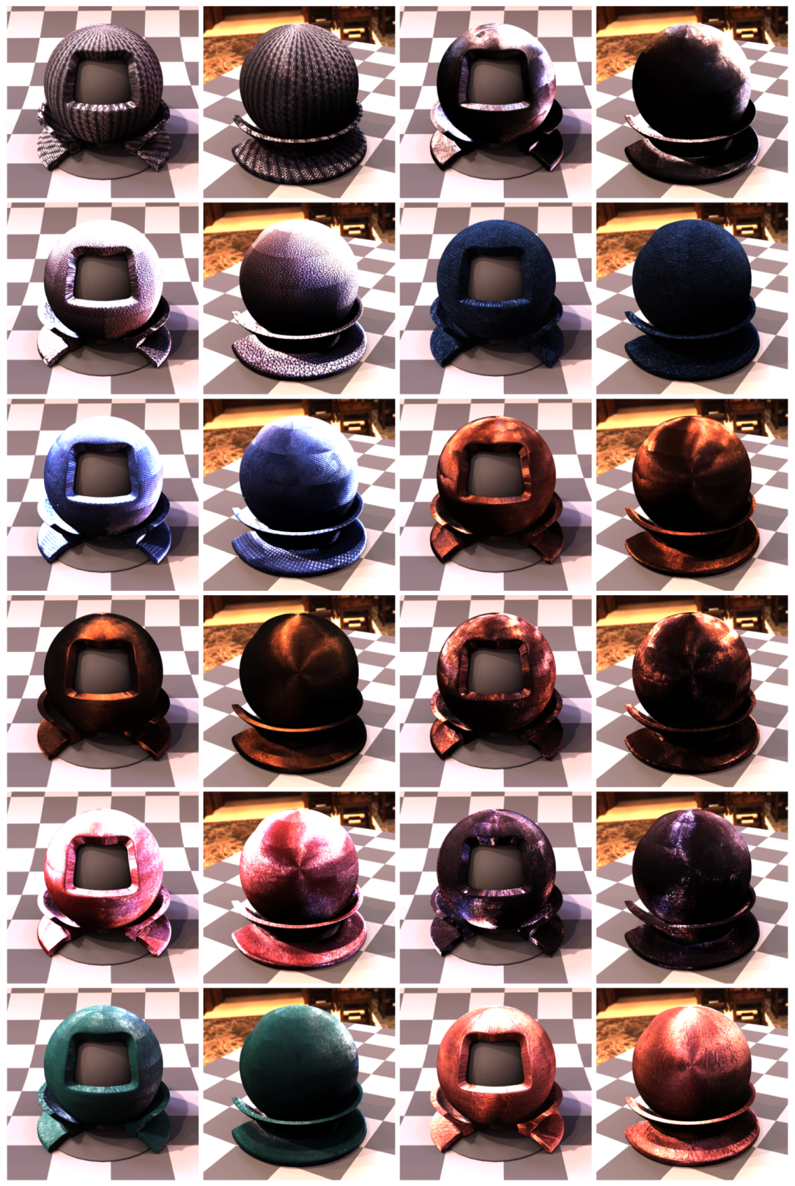
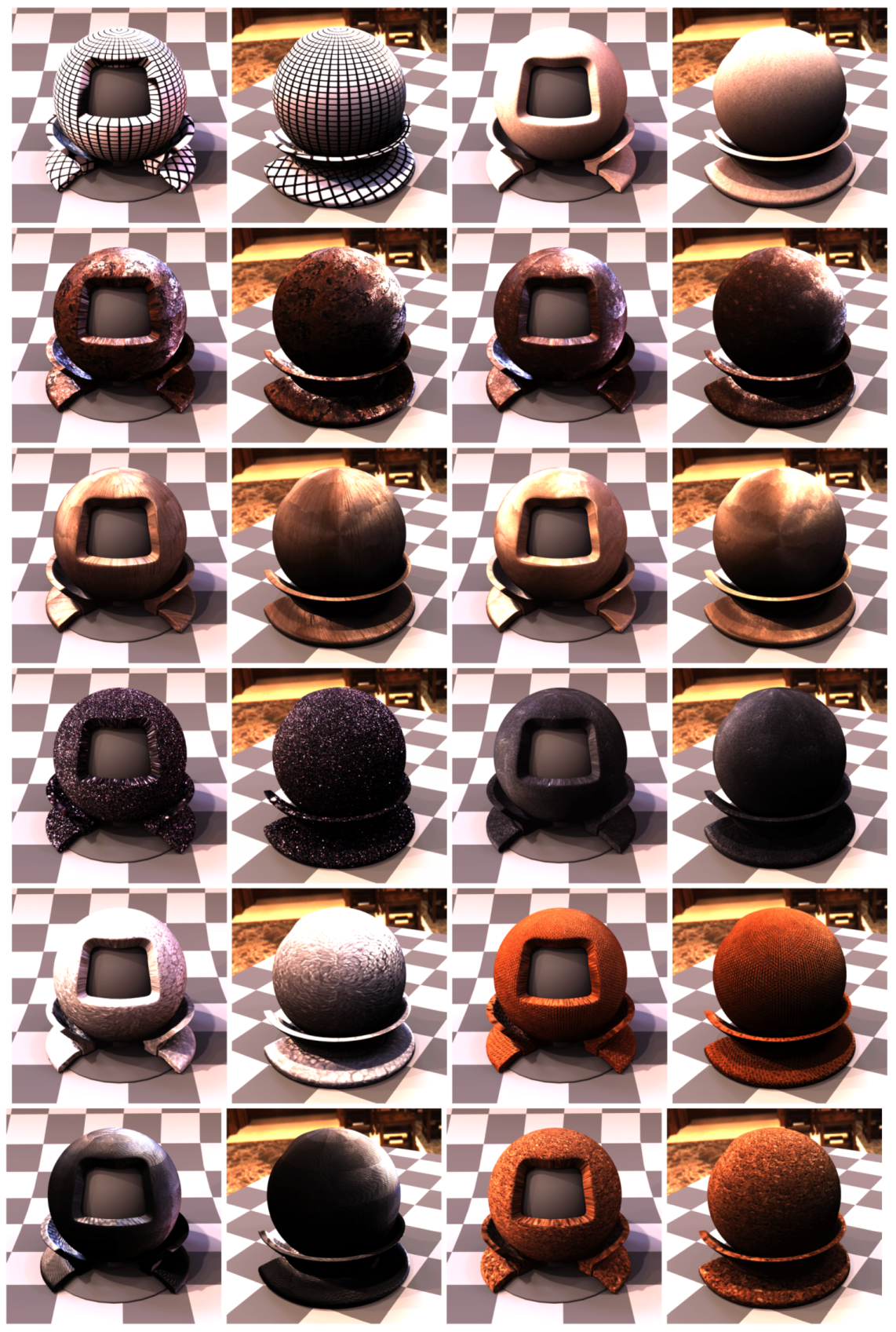
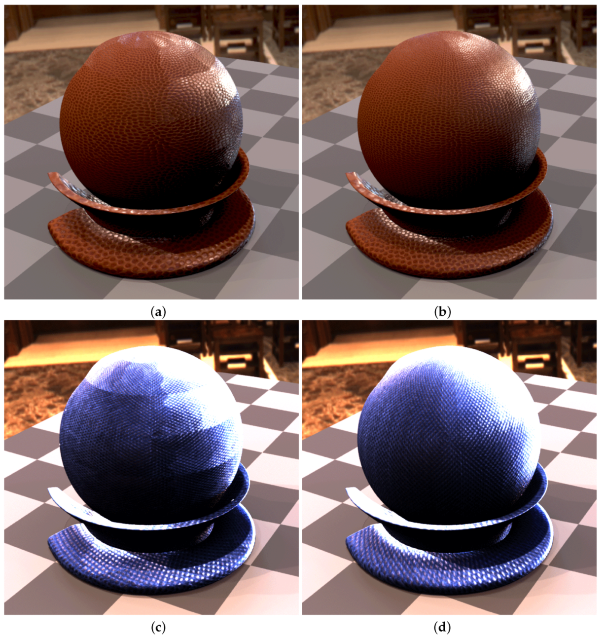
12. Results
12.1. Software
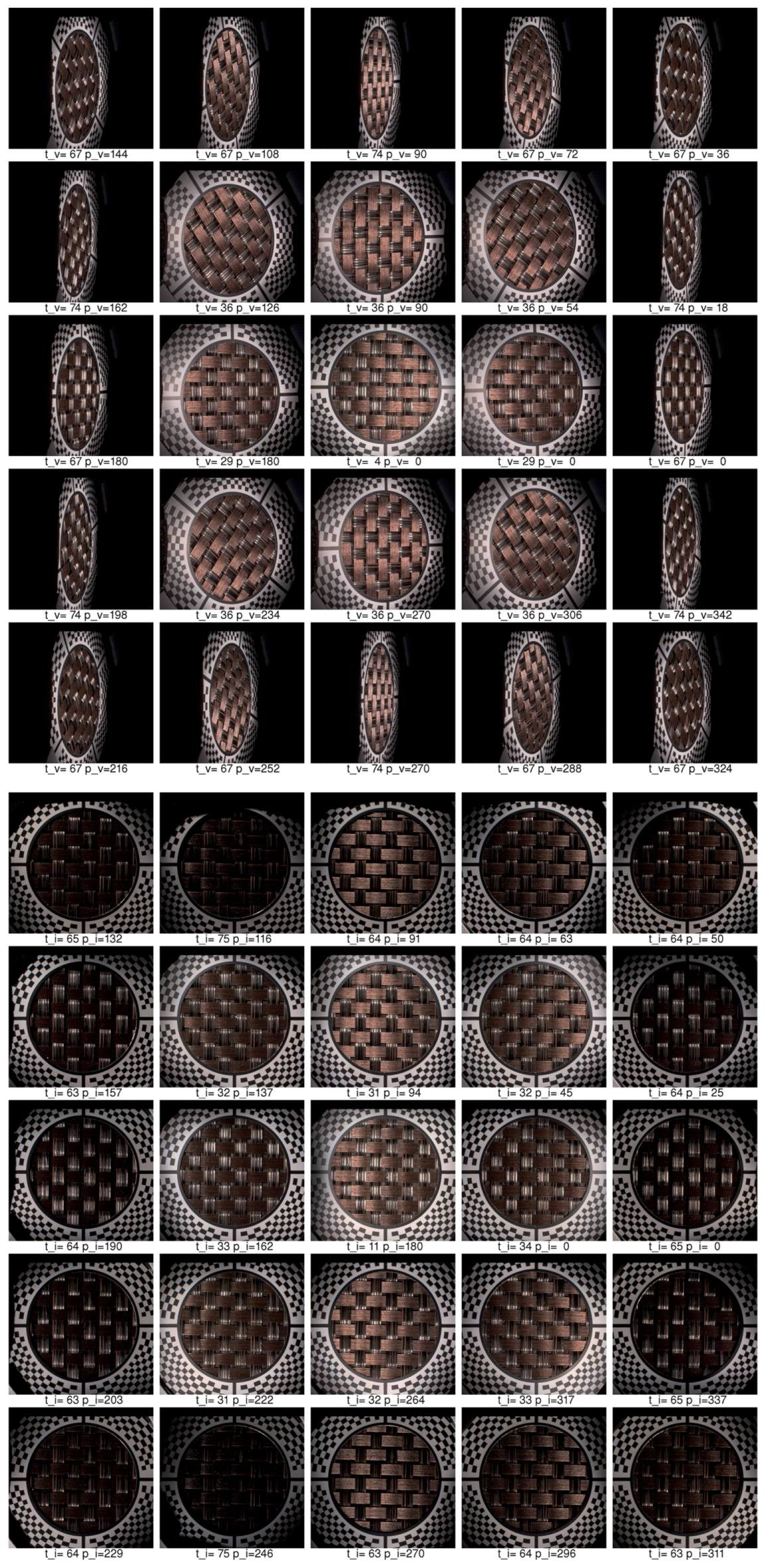
12.2. Measurements
12.3. MAM 2014 Sample Set Measurements
12.4. Data Processing
12.5. Rendering
12.6. Comparison
12.7. Data and Videos
13. Limitations
13.1. Optical and Spatial Limitations
13.2. Camera Limitations
13.3. Angular Limitations of Illumination
13.4. Highly Glossy BTF
13.5. Construction and Environmental Limitations
13.6. Other Limitations
14. Conclusions
Supplementary Materials
Acknowledgments
Author Contributions
Conflicts of Interest
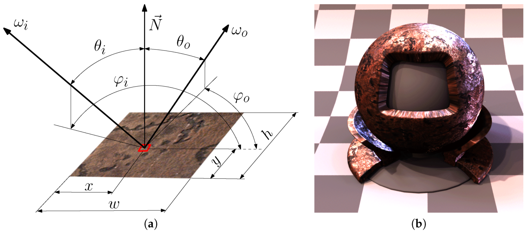
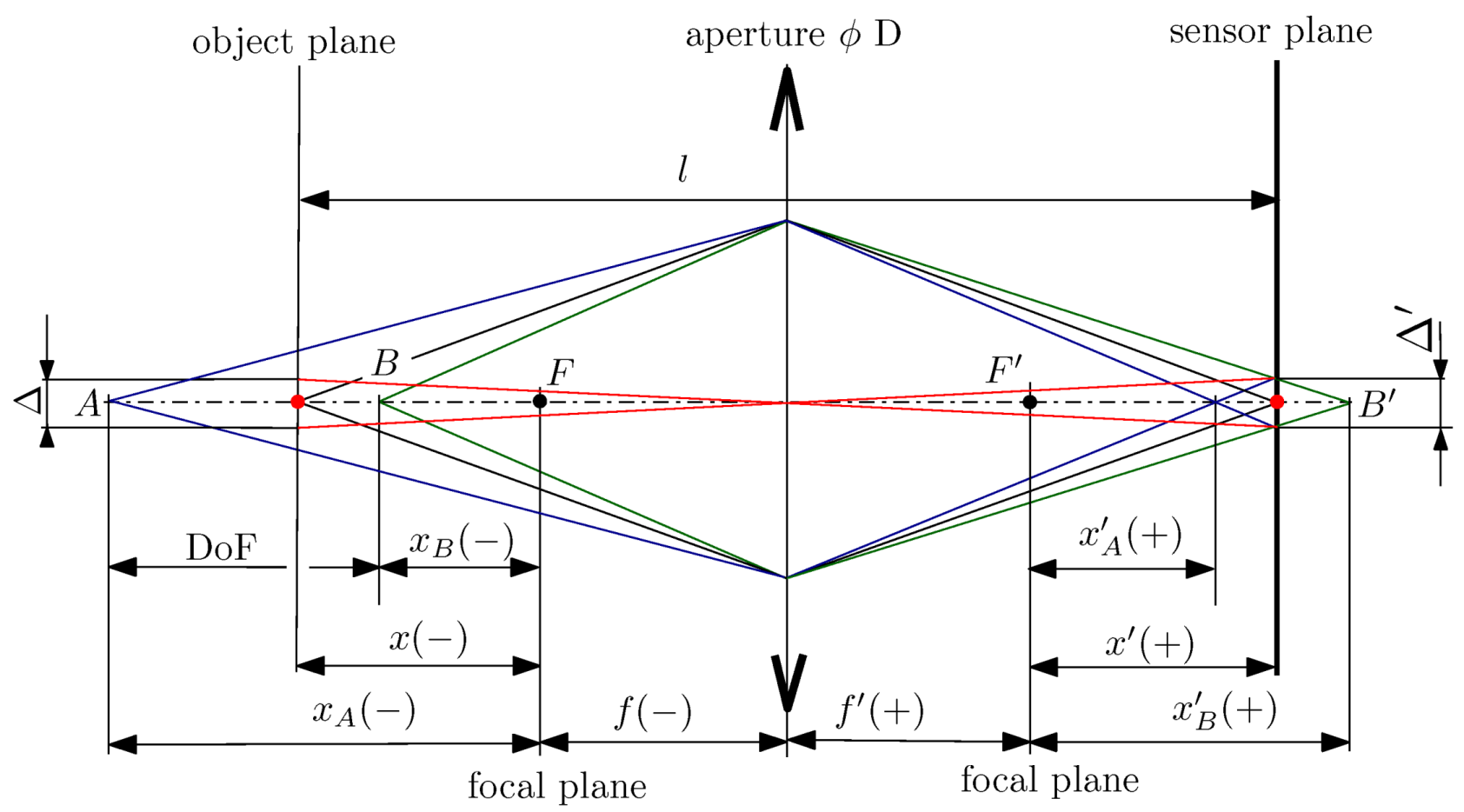
Appendix A. DoF Derivation for BTF Instrument with Thin Lens Imaging
Appendix B. Geometric Uncertainty and Accuracy of Illumination and Cameras
Appendix B.1. Evaluation of Angular Position Uncertainty of Illumination Source

| Illumination Alignment Uncertainty | Meridional Direction | Zonal Direction |
|---|---|---|
| LED chip soldered to the platform | mm | mm |
| LED chip inclination | 0–15 | 0–15 |
| LED chip inclination compensated | ||
| with condenser decentration | 20–2.6 mm | 20–2.6 mm |
| adjustment screws clearance | mm | mm |
| adjustable platform alignment range | ||
| LED chip shift by adjustment | mm | mm |
| liner clearance in the dome hole | mm | mm |
| dome misalignment during machining | mm | mm |
| dome inclination towards sample | ||
| dome misalignment towards sample | mm | mm |
Appendix B.2. Evaluation of Angular Position Uncertainty of Cameras
| Camera Alignment Uncertainty | Meridional Direction | Zonal Direction |
|---|---|---|
| camera mount on adjustable platform | mm | mm |
| adjustment screws clearance | mm | mm |
| adjustable platform alignment range | ||
| camera shift by adjustment | mm | mm |
| fixtures mount on the arm | mm | mm |
| linear guide clearance | - | mm |
| threaded screw axial end play | mm | - |
| frame’s leg mounting position | mm | mm |
| inner aluminium frame misalignment during machining | mm | mm |
| inner aluminium frame inclination towards sample | ||
| inner aluminium frame misalignment towards sample | mm | mm |
Appendix C. Marker Sticker Code Listing in ANSI C++ Language
  1 // The source code written by Vlastimil Havran, September 2015
  2 #include <cstdlib>
  3 #include <iostream>
  4 #include <fstream>
  5 #include <cmath>
  6 #include "Board.h"
  7
  8 using namespace LibBoard;
  9 using namespace std;
 10
 11 #define MIDCOLOR 0,255,0
 12
 13 // Positive - printing black on white background
 14 #define WHITE 255,255,255
 15 #define BLACK 0,0,0
 16 #define NOINVERT 1
 17 #define HOLE 1
 18
 19 inline float sqr(float a) { return a*a;}
 20
 21 // From Libboard library https://github.com/c-koi/libboard by Sebastien Fourey
 22 Board board;
 23
 24 void PutRectangle(float centerx, float centery, float width, float height)
 25 {
 26   board.fillRectangle(centerx-width/2.0, centery+height/2.0, width, height);
 27 }
 28
 29 int CropPoint(Point &p1, float mSize)
 30 {
 31   int cnt = 0;
 32   float dist = sqrt(p1.x*p1.x + p1.y*p1.y);
 33   float maxdist = sqrt(2.0)*mSize;
 34   bool crop = false;
 35   if (p1.x > mSize) {crop = true;}
 36   if (p1.x < -mSize) {crop = true;}
 37   if (p1.y > mSize) {crop = true;}
 38   if (p1.y < -mSize) {crop = true;}
 39
 40   if (crop) { // Find the closest point to the center in the square
 41     int cnt = 10000;
 42     for (int i = cnt; i ; i–) {
 43       float mult = (float)i/(float)cnt;
 44       Point pp = p1;
 45       pp.x *= mult;
 46       pp.y *= mult;
 47       bool crop2 = false;
 48       if (pp.x > mSize) {crop2 = true;}
 49       if (pp.x < -mSize) {crop2 = true;}
 50       if (pp.y > mSize) {crop2 = true;}
 51       if (pp.y < -mSize) {crop2 = true;}
 52       if (!crop2) {
 53         p1 = pp;
 54         return true; // was cropped
 55       }
 56     }
 57   }
 58   return false;
 59 }
 60
 61 int CropPointXY1(Point &pp, float mSizeX, float mSizeY)
 62 {
 63   int cnt = 0;
 64   if ((pp.x < mSizeX)&&(pp.y < mSizeY))
 65     cnt++;
 66   return cnt;
 67 }
 68
 69 int CropPointXY2(Point &pp, float mSizeX, float mSizeY)
 70 {
 71   int cnt = 0;
 72   if ((pp.x > mSizeX)&&(pp.y < mSizeY))
 73     cnt++; // inside;
 74   return cnt;
 75 }
 76
 77 bool CMP(float phi, float endPhi, int q)
 78 {
 79   if ((q % 2) == 0)
 80     return phi < endPhi;
 81   return phi > endPhi;
 82 }
 83
 84 template<class T> void Swap(T &x, T &y) { T temp = x; x = y; y = temp;}
 85
 86 int main(int argc, char *argv[])
 87 {
 88   board.clear( Color(WHITE) );
 89   float mSize = 85.f; // mm - size of marker
 90
 91   board.setLineWidth( 12.5 ).setPenColorRGBi( WHITE );
 92   board.setLineStyle( Shape::SolidStyle );
 93   board.setLineJoin( Shape::MiterJoin );
 94   board.setLineCap( Shape::RoundCap );
 95
 96   // Draw a frame around the image - black
 97   board.setLineWidth( 4.0 ).setPenColorRGBi( BLACK );
 98   board.drawRectangle(-0.5, 0.5, 1.0, 1.0);
 99   // Draw a small frame right bottom
100   board.setLineWidth( 1.5 ).setPenColorRGBi( BLACK );
101   board.drawRectangle(0.325, -0.43, 0.175, 0.07);
102   // Draw a small frame left bottom
103   board.setLineWidth( 1.5 ).setPenColorRGBi( BLACK );
104   board.drawRectangle(-0.5, -0.43, 0.092, 0.07);
105
106   // chequerboard pattern in polar coordinates
107   float deltaPhi = 2.9*M_PI/(64.0)/2.0; // radians
108   float deltaRad = 4.3f/mSize/2.0; // mm
109   const float phiStartOffset = 0.1f;
110   const float phiEndOffset = 0.08f;
111   // Each quarter part of radial chequerboard patttern has its own data
112   for (int q = 0; q < 4; q++) {
113     int odd2 = 0;
114     float begPhi, endPhi, stepPhi;
115     // Set initial conditions
116     if (q == 0) {
117       begPhi = phiStartOffset;
118       endPhi = M_PI/2.0 - phiEndOffset;
119       stepPhi = deltaPhi;
120     }
121     if (q == 1) {
122       begPhi = M_PI - phiStartOffset;
123       endPhi = M_PI/2.0f + phiEndOffset;
124       stepPhi = -deltaPhi;
125     }
126     if (q == 2) {
127       begPhi = M_PI + phiStartOffset;
128       endPhi = 3.0/2.0*M_PI - phiEndOffset;
129       stepPhi = deltaPhi;
130     }
131     if (q == 3) {
132       begPhi = 2.0*M_PI - phiStartOffset;
133       endPhi = 3.0/2.0*M_PI + phiEndOffset;
134       stepPhi = -deltaPhi*1.05;
135     }
136
137     // Increasing phi
138     for (float phi = begPhi; CMP(phi+stepPhi, endPhi, q); phi += stepPhi, odd2++) {
139      if (q == 0)
140         stepPhi *= 1.03f;
141       if (q == 1)
142         stepPhi = -deltaPhi*1.3 - deltaPhi*0.3*sin((phi-begPhi)*3.5 + M_PI*2.0f/4.0);
143       if (q == 2)
144         stepPhi = deltaPhi*1.3 + deltaPhi*0.3*sin((phi-begPhi)*5.0 + M_PI*1.25f/4.0);
145       if (q == 3)
146         stepPhi = -deltaPhi*1.3 + deltaPhi*0.3*cos((phi-begPhi)*5.5 + M_PI*1.25f/4.0);
147       int odd = 0; // if to start with black or white region of chequerboard pattern
148       if ((odd2%2) == 0) odd = 1;
149       // Increasing radius by a fixed step
150       for (float rad = 28.5/mSize; rad < 0.61; rad += deltaRad) {
151         int cnt = 0;
152         // 4 corners defining the radial region of the chequerboard pattern element
153         Point p1(rad*cos(phi), rad*sin(phi));
154         Point p2((rad+deltaRad)*cos(phi), (rad+deltaRad)*sin(phi));
155         Point p3((rad+deltaRad)*cos(phi+stepPhi), (rad+deltaRad)*sin(phi+stepPhi));
156         Point p4(rad*cos(phi+stepPhi), rad*sin(phi+stepPhi));
157         if ((q == 1) || (q==3)) {
158           Swap(p2, p3);
159           Swap(p1, p4);
160         }
161         float maxf = 0.487;
162         cnt += CropPoint(p1, maxf);
163         cnt += CropPoint(p2, maxf);
164         cnt += CropPoint(p3, maxf);
165         cnt += CropPoint(p4, maxf);
166         float phi2 = atan2(p2.y, p2.x);
167         float phi3 = atan2(p3.y, p3.x);
168
169         float th = 0.004f;
170         float maxcheck = 0.48f;
171         if ( (q==0) && (p1.x > maxcheck) && (fabs(p1.x - p2.x) < th) &&
172              (fabs(p2.x - p3.x) < th) && (fabs(p4.x - p3.x) < th) ) continue;
173         if ( (q==0) && (p1.y > maxcheck) && (fabs(p1.y - p2.y) < th) &&
174              (fabs(p2.y - p3.y) < th) && (fabs(p4.y - p3.y) < th) ) continue;
175         if ( (q==1) && (p1.x < -maxcheck) && (fabs(p1.x - p2.x) < th) &&
176              (fabs(p2.x - p3.x) < th) && (fabs(p4.x - p3.x) < th) ) continue;
177         if ( (q==1) && (p1.y > maxcheck) && (fabs(p1.y - p2.y) < th) &&
178              (fabs(p2.y - p3.y) < th) && (fabs(p4.y - p3.y) < th) ) continue;
179         if ( (q==2) && (p1.x < -maxcheck) && (fabs(p1.x - p2.x) < th) &&
180              (fabs(p2.x - p3.x) < th) && (fabs(p4.x - p3.x) < th) ) continue;
181         if ( (q==2) && (p1.y < -maxcheck) && (fabs(p1.y - p2.y) < th) &&
182              (fabs(p2.y - p3.y) < th) && (fabs(p4.y - p3.y) < th) ) continue;
183         if ( (q==3) && (p1.x > maxcheck) && (fabs(p1.x - p2.x) < th) &&
184              (fabs(p2.x - p3.x) < th) && (fabs(p4.x - p3.x) < th) ) continue;
185         if ( (q==3) && (p1.y < -maxcheck) && (fabs(p1.y - p2.y) < th) &&
186              (fabs(p2.y - p3.y) < th) && (fabs(p4.y - p3.y) < th) ) continue;
187
188         if (cnt < 8) { // We have not cropped the whole region, draw it
189           // Avoid right bottom corner
190           const float bottomDistMarkY1 = -0.43;
191           const float bottomDistMarkX1 = 0.36;
192           int cnt2 = CropPointXY2(p1, bottomDistMarkX1, bottomDistMarkY1);
193           cnt2 += CropPointXY2(p2, bottomDistMarkX1, bottomDistMarkY1);
194           cnt2 += CropPointXY2(p3, bottomDistMarkX1, bottomDistMarkY1);
195           cnt2 += CropPointXY2(p4, bottomDistMarkX1, bottomDistMarkY1);
196           if (cnt2 > 0) {
197             continue;
198           }
199           // Avoid left bottom corner
200           const float bottomDistMarkY2 = -0.43;
201           const float bottomDistMarkX2 = -0.42;
202           cnt2 = 0;
203           cnt2 += CropPointXY1(p1, bottomDistMarkX2, bottomDistMarkY2);
204           cnt2 += CropPointXY1(p2, bottomDistMarkX2, bottomDistMarkY2);
205           cnt2 += CropPointXY1(p3, bottomDistMarkX2, bottomDistMarkY2);
206           cnt2 += CropPointXY1(p4, bottomDistMarkX2, bottomDistMarkY2);
207           if (cnt2 > 0) {
208             odd = !odd;
209             continue;
210          }
211           // Draw a filed polygon of polar chequerboard region in black
212           vector<Point> polyline;
213           // First vertex p1
214           polyline.push_back(p1);
215           cnt2 = 200; // how finely decompose arc to line segments
216           // From p2 to p3
217           float rad1 = sqrt(p2.x*p2.x + p2.y*p2.y);
218           float rad2 = sqrt(p3.x*p3.x + p3.y*p3.y);
219           float phi1 = atan2(p2.y, p2.x);
220           float phi2 = atan2(p3.y, p3.x);
221           int i = 0;
222           if (phi2 > phi1) {
223             for (float p = phi1; p < phi2; p += (phi2-phi1)/(float)cnt2, i++) {
224               float alpha = (float)i/(float)cnt2;
225               float r = rad1*(1.0 - alpha) + rad2*alpha;
226               Point pp(r*cos(p), r*sin(p));
227               polyline.push_back(pp);
228             }
229           } else {
230             for (float p = phi1; p > phi2; p -= (phi1-phi2)/(float)cnt2, i++) {
231               float alpha = (float)i/(float)cnt2;
232               float r = rad1*(1.0 - alpha) + rad2*alpha;
233               Point pp(r*cos(p), r*sin(p));
234               polyline.push_back(pp);
235             } // for i
236           }
237           polyline.push_back(p3);
238           // From p4 to p1
239           rad1 = sqrt(p4.x*p4.x + p4.y*p4.y);
240           rad2 = sqrt(p1.x*p1.x + p1.y*p1.y);
241           phi1 = atan2(p4.y, p4.x);
242           phi2 = atan2(p1.y, p1.x);
243           i = 0;
244           if (phi2 > phi1) {
245             for (float p = phi1; p < phi2; p += (phi2-phi1)/(float)cnt2, i++) {
246               float alpha = (float)i/(float)cnt2;
247               float r = rad1*(1.0 - alpha) + rad2*alpha;
248               Point pp(r*cos(p), r*sin(p));
249               polyline.push_back(pp);
250             }
251           } else {
252             for (float p = phi1; p > phi2; p -= (phi1-phi2)/(float)cnt2, i++) {
253               float alpha = (float)i/(float)cnt2;
254               float r = rad1*(1.0 - alpha) + rad2*alpha;
255               Point pp(r*cos(p), r*sin(p));
256               polyline.push_back(pp);
257             } // for i
258           }
259           if (odd) // draw only black regions of polar chequerboard pattern
260             board.fillPolyline(polyline, -1);
261         }
262         odd = !odd; // change the order of black and white the next time
263       } // rad
264     } // phi
265   } // for q
266
267   // Add four rectangles to represent cross hair
268   float bw = 0.02;
269   float bh = 0.18;
270   const float offsetMark = 0.40;
271   float kw = 1.0;
272   float kh = 1.0;
273   // top middle
274   PutRectangle(0.0, offsetMark, bw*kw, bh*kh);
275   // bottom middle
276   PutRectangle(0.0, -offsetMark, bw*kw, bh*kh);
277   // right middle
278   PutRectangle(offsetMark, 0, bh*kh, bw*kw);
279   // left middle
280   PutRectangle(-offsetMark, 0, bh*kh, bw*kw);
281
282   const float RADIUS = 23.5; // mm
283   const float RADIUS2 = 20.0; // mm
284   const float RADIUS3 = 51.0/2.0f; // mm
285   // Draw the important circle by black color
286   if (!HOLE) {
287     if (NOINVERT) {
288       // black
289       board.setLineWidth( RADIUS2 ).setPenColorRGBi( BLACK );
290       board.drawCircle(0, 0, 1.00*RADIUS/mSize, -1);
291     }
292     else {
293       float RADIUS3 = RADIUS + RADIUS2/6.0 + 0.215f;
294       board.setLineWidth(0.f).setPenColorRGBi( BLACK );
295       board.fillCircle(0, 0, RADIUS3/mSize,-1);
296     }
297   } else {
298     // Make a hole in special color
299     board.setLineWidth( RADIUS2 ).setPenColorRGBi( BLACK );
300     board.drawCircle(0, 0, 1.00*RADIUS/mSize,-1);
301     board.setLineWidth(0.f).setPenColorRGBi( MIDCOLOR );
302     board.fillCircle(0, 0, RADIUS3/mSize,-1);
303   }
304
305   // Draw a cross in the middle of the sticker - black
306   if (NOINVERT) {
307     // This makes no sense for a sticker production company
308     board.setLineWidth( 0.5 ).setPenColorRGBi( BLACK );
309     float deltaCross = 0.04f;
310     board.drawLine( -deltaCross, 0, deltaCross, 0);
311     board.drawLine( 0, -deltaCross, 0, deltaCross);
312   }
313
314   board.setPenColor( Color(BLACK) ).setFont( Fonts::HelveticaBold, 5.5 )
315     .drawText( -0.488, 0.440, "FEL FSI" );
316   board.setPenColor( Color(BLACK) ).setFont( Fonts::HelveticaBold, 5.5 )
317     .drawText( -0.488, 0.466, "CVUT" );
318   board.setPenColor( Color(BLACK) ).setFont( Fonts::HelveticaBold, 5.5 )
319     .drawText( 0.380, 0.466, "HAVRAN" );
320
321   // 85x85mm - final size of EPS/FIG/SVG
322   board.saveEPS("markersticker.eps", mSize, mSize, 0);
323   return 0;
324 }
Appendix D. Gantry Assembly


References
- Nicodemus, F.E.; Richmond, J.C.; Hsia, J.J.; Ginsberg, I.W.; Limperis, T. Geometric Considerations and Nomenclature for Reflectance; Monograph 161, National Bureau of Standards (US); Jones and Bartlett Publishers: Burlington, MA, USA, 1977. [Google Scholar]
- Dana, K.; Van-Ginneken, B.; Nayar, S.; Koenderink, J. Reflectance and Texture of Real World Surfaces. ACM Trans. Graph. 1999, 18, 1–34. [Google Scholar] [CrossRef]
- Dana, K.J.; Nayar, S.K.; van Ginneken, B.; Koenderink, J.J. Reflectance and Texture of Real-World Surfaces. In Proceedings of the IEEE Computer Society Conference on Computer Vision and Pattern Recognition, San Juan, Puerto Rico, 17–19 June 1997; pp. 151–157.
- Schwartz, C.; Sarlette, R.; Weinmann, M.; Rump, M.; Klein, R. Design and Implementation of Practical Bidirectional Texture Function Measurement Devices Focusing on the Developments at the University of Bonn. Sensors 2014, 14, 7753–7819. [Google Scholar] [CrossRef] [PubMed]
- Filip, J.; Haindl, M. Bidirectional Texture Function Modeling: A State of the Art Survey. IEEE Trans. Pattern Anal. Mach. Intell. 2009, 31, 1921–1940. [Google Scholar] [CrossRef] [PubMed]
- Weyrich, T.; Lawrence, J.; Lensch, H.; Rusinkiewicz, S.; Zickler, T. Principles of Appearance Acquisition and Representation. Found. Trends Comput. Graph. Vis. 2008, 4, 75–191. [Google Scholar] [CrossRef]
- Müller, G.; Meseth, J.; Sattler, M.; Sarlette, R.; Klein, R. Acquisition, Synthesis, and Rendering of Bidirectional Texture Functions. Comput. Graph. Forum 2005, 24, 83–109. [Google Scholar] [CrossRef]
- Weinmann, M.; Klein, R. Advances in Geometry and Reflectance Acquisition (Course Notes). In SIGGRAPH Asia 2015 Courses; ACM: New York, NY, USA, 2015; pp. 1:1–1:71. [Google Scholar]
- Riviere, J.; Peers, P.; Ghosh, A. Mobile Surface Reflectometry. Comput. Graph. Forum 2016, 35, 191–202. [Google Scholar] [CrossRef]
- Aittala, M.; Weyrich, T.; Lehtinen, J. Practical SVBRDF Capture in the Frequency Domain. ACM Trans. Graph. 2013, 32, 110:1–110:12. [Google Scholar] [CrossRef]
- Dana, K. BRDF/BTF Measurement Device. In Proceedings of the Eighth IEEE International Conference on Computer Vision, Vancouver, BC, Canada, 7–14 July 2001; Volume 2, pp. 460–466.
- Han, J.Y.; Perlin, K. Measuring Bidirectional Texture Reflectance with a Kaleidoscope. ACM Trans. Graph. 2003, 22, 741–748. [Google Scholar] [CrossRef]
- Ben-Ezra, M.; Wang, J.; Wilburn, B.; Li, X.; Ma, L. An LED-Only BRDF Measurement Device. In Proceedings of the IEEE Conference on Computer Vision and Pattern Recognition (CVPR 2008), Anchorage, AK, USA, 23–28 June 2008; IEEE Computer Society: Los Alamitos, CA, USA, 2008; pp. 1–8. [Google Scholar]
- Debevec, P.; Hawkins, T.; Tchou, C.; Duiker, H.P.; Sarokin, W.; Sagar, M. Acquiring the Reflectance Field of a Human Face. In Proceedings of the 27th Annual Conference on Computer Graphics and Interactive Techniques, Seattle, WA, USA, 14–18 July 1980; ACM Press: New York, NY, USA, 2000; pp. 145–156. [Google Scholar]
- Malzbender, T.; Gelb, D.; Wolters, H. Polynomial Texture Maps. In Proceedings of the 28th Annual Conference on Computer Graphics and Interactive Techniques, Los Angeles, CA, USA, 12–17 August 2001; ACM: New York, NY, USA, 2001; pp. 519–528. [Google Scholar]
- Foo, S.C. A Gonioreflectometer for Measuring the Bidirectional Reflectance of Material for Use in Illumination Computation. Master’s Thesis, Cornell University, Ithaca, NY, USA, August 1997. [Google Scholar]
- Sattler, M.; Sarlette, R.; Klein, R. Efficient and Realistic Visualization of Cloth. In Proceedings of the 14th Eurographics Workshop on Rendering, Leuven, Belgium, 25–26 June 2003; Eurographics Association: Aire-la-Ville, Switzerland, 2003; pp. 167–177. [Google Scholar]
- Huenerhoff, D.; Grusemann, U.; Hope, A. New robot-based gonioreflectometer for measuring spectral diffuse reflection. Metrologia 2006, 43, S11. [Google Scholar] [CrossRef]
- Schwartz, C.; Sarlette, R.; Weinmann, M.; Klein, R. DOME II: A Parallelized BTF Acquisition System. In Proceedings of the Eurographics 2013 Workshop on Material Appearance Modeling, Issues and Acquisition, MAM ’13, Zaragoza, Spain, 19 June 2013; Eurographics Association: Aire-la-Ville, Switzerland, 2013; pp. 25–31. [Google Scholar]
- Köhler, J.; Noll, T.; Reis, G.; Stricker, D. A Full-Spherical Device for Simultaneous Geometry and Reflectance Acquisition. In Proceedings of the 2013 IEEE Workshop on Applications of Computer Vision, Clearwater Beach, FL, USA, 15–17 January 2013; pp. 355–362.
- Filip, J.; Vávra, R.; Krupička, M. Rapid Material Appearance Acquisition Using Consumer Hardware. Sensors 2014, 14, 19785–19805. [Google Scholar] [CrossRef] [PubMed]
- Hošek, J.; Havran, V.; Čáp, J.; Němcová, S.; Macúchová, K.; Bittner, J.; Zicha, J. Realisation of Circular Motion for Portable BTF Measurement Instrument. Romanian Rev. Precis. Mech. Opt. Mechatron. 2015, 48, 252–255. [Google Scholar]
- Tong, X.; Wang, J.; Lin, S.; Guo, B.; Shum, H.Y. Modeling and rendering of quasi-homogeneous materials. ACM Trans. Graph. 2005, 24, 1054–1061. [Google Scholar] [CrossRef]
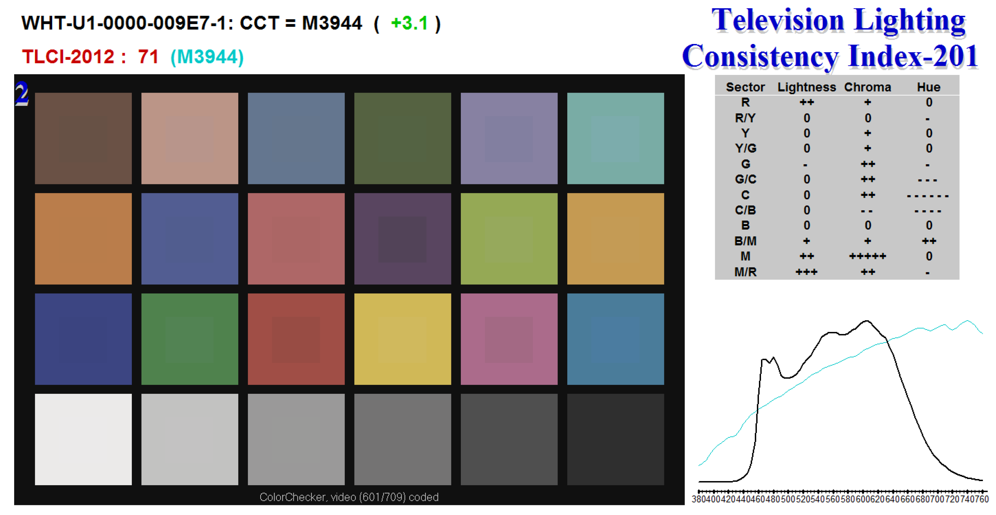
- CIE 13.3-95. Method of Measuring and Specifying Colour Rendering Properties of Light Sources, Publication 13.3-1995. In A Verbatim Re-Publication of the 1974, 2nd ed.; Commission Internationale de l’Eclairage: Vienna, Austria, 1995. [Google Scholar]
- CIE 177:2007. CIE Technical Report 177:2007, Color Rendering of White LED Light Sources; Commission Internationale de l’Eclairage: Vienna, Austria, 2007. [Google Scholar]
- EBU. TECH 3355—Method for the Assesment of the Colorimetric Properties of Luminaires—The Television Lighting Consistency Index (TLCI-2012); EBU: Geneva, Switzerland, 2014. [Google Scholar]
- Lloyd, S. Least Squares Quantization in PCM. IEEE Trans. Inf. Theory 2006, 28, 129–137. [Google Scholar] [CrossRef]
- Vávra, R.; Filip, J. Registration of Multi-View Images of Planar Surfaces. In Proceedings of the 11th Asian Conference on Computer Vision, ACCV, Daejeon, Korea, 5–9 November 2012.
- Havran, V. Practical Experiences with Using Autocollimator for Surface Reflectance Measurement. In Workshop on Material Appearance Modeling; Klein, R., Rushmeier, H., Eds.; The Eurographics Association: Geneva, Switzerland, 2016. [Google Scholar]
- Billinghurst, M.; Clark, A.; Lee, G. A Survey of Augmented Reality. Found. Trends Hum. Comput. Interact. 2015, 8, 73–272. [Google Scholar] [CrossRef]
- Haindl, M.; Filip, J. Visual Texture. In Advances in Computer Vision and Pattern Recognition; Springer: London, UK, 2013. [Google Scholar]
- Press, W.H.; Teukolsky, S.A.; Vetterling, W.T.; Flannery, B.P. Numerical Recipes in C++; Cambridge University Press: Cambridge, UK, 2002. [Google Scholar]
- Evangelidis, G.D.; Psarakis, E.Z. Parametric Image Alignment Using Enhanced Correlation Coefficient Maximization. IEEE Trans. Pattern Anal. Mach. Intell. 2008, 30, 1858–1865. [Google Scholar] [CrossRef] [PubMed]
- Bradski, G.; Kaehler, A. Learning OpenCV: Computer Vision in C++ with the OpenCV Library, 2nd ed.; O’Reilly Media, Inc.: Sebastopol, CA, USA, 2013. [Google Scholar]
- Rushmeier, H. The MAM2014 Sample Set. In Eurographics Workshop on Material Appearance Modeling; Klein, R., Rushmeier, H., Eds.; The Eurographics Association: Geneva, Switzerland, 2014. [Google Scholar]
- Müller, G.; Meseth, J.; Klein, R. Compression and Real-Time Rendering of Measured BTFs Using Local PCA. In Vision, Modeling and Visualisation 2003; Ertl, T., Girod, B., Greiner, G., Niemann, H., Seidel, H.P., Steinbach, E., Westermann, R., Eds.; Akademische Verlagsgesellschaft Aka GmbH: Berlin, Germany, 2003; pp. 271–280. [Google Scholar]
- Haindl, M.; Hatka, M. A Roller—Fast Sampling-Based Texture Synthesis Algorithm. In Proceedings of the 13th International Conference in Central Europe on Computer Graphics, Visualization and Computer Vision 2005, Bory, Czech Republic, 31 January–4 February 2005; Skala, V., Ed.; University of Western Bohemia: Plzen, Czech Republic, 2005; pp. 80–83. [Google Scholar]
- Jakob, W. Mitsuba Renderer. 2010. Available online: http://www.mitsuba-renderer.org (accessed on 20 May 2016).
- Havran, V.; Neummann, A.; Zotti, G.; Purgathofer, W.; Seidel, H.P. On Cross-Validation and Resampling of BRDF Data Measurements. In Proceedings of the 21st Spring Conference on Computer Graphics (SCCG 2005), Budmerice, Slovakia, 12–14 May 2005; Juettler, B., Ed.; ACM SIGGRAPH and EUROGRAPHICS, 2005; pp. 154–161. [Google Scholar]
- Ruiters, R.; Schwartz, C.; Klein, R. Example-Based Interpolation and Synthesis of Bidirectional Texture Functions. Comput. Graph. Forum 2013, 32, 361–370. [Google Scholar] [CrossRef]


| Parameter/Setup | Dome 1 | Dome 2 | Lightdrum | |
|---|---|---|---|---|
| Configuration (Year) | 2004 | 2008/2011 | 2012 | 2016 |
| dimensions (L × W × H) [mm] | ||||
| distance to sample [mm] | 650 | 1000 | 251 | |
| directions | ||||
| resolution | 9.4 | 9 | 11.1 | |
| resolution | 9.4 | 7.6 | 10.1 | |
| maximum θ | 75 | 75 | 75 | |
| equivalent focal length [mm] | 116 | 104 | 190/95 | 80 |
| focal length [mm] | 16.22 | 22 | 100/50 | 12.5 |
| spatial resolution [DPI] | 235 | 450 | 380/190 | 300/150 |
| dynamic range [dB] | 28/33/33 | 25/44/44 | 32/60/∞ | 60.06/78.06/- |
| spectral bands | RGB | RGB | RGB | |
| camera type | Canon P&S | Industrial CCD | Industrial CMOS | |
| camera sensor size [mm] | ||||
| camera sensor pixel resolution | ||||
| #cameras | 151 | 11 | 6 | |
| camera data | 8 BPP JPEG | 12 BPP raw | 12 BPP raw | |
| light source type | flash | LED | LED | |
| #light sources | 151 | 198 | 139 | |
| measurement size [mm] | ⊘ 51 | |||
| direction variation (field of view) | ||||
| BTF raw/HDR images | 91,204/22,801 | 156,816/52,272 | 66,720/16,680 | |
| saved HDR images resolution | ||||
| equivalent BTF HDR size [GB] | 200 | 764 | 612 | 40 |
| BTF size (disk space) [GB] | 22 | 281 | 918 | 40 |
| BTF time [h] | 1.8 | 4.4–9.7 | 0.28 | |
| HDR speed [Msamples/s] | 10.56 | 40.27 | 6–13.2 | 12.58 |
| radiometric repeatability | - | 7.4 | 0.1 | <0.6 |
| geometric repeatability | - | 0.81 px/0.006 | 0.12 px/0.002 | 1.20 px/0.011 |
| and ±0.05 px/0.002 | ||||
| sample flexibility | none | some; arbitrary | arbitrary , dependent | |
| radiometric calib. procedure | complex | easy | easy | |
| geometric calib. procedure | automatic | automatic | automatic | |
| durability (#measurements) | - | ≈265/>347 | >3650 | >20,000 |
© 2017 by the authors. Licensee MDPI, Basel, Switzerland. This article is an open access article distributed under the terms and conditions of the Creative Commons Attribution (CC BY) license ( http://creativecommons.org/licenses/by/4.0/).
Share and Cite
Havran, V.; Hošek, J.; Němcová, Š.; Čáp, J.; Bittner, J. Lightdrum—Portable Light Stage for Accurate BTF Measurement on Site. Sensors 2017, 17, 423. https://doi.org/10.3390/s17030423
Havran V, Hošek J, Němcová Š, Čáp J, Bittner J. Lightdrum—Portable Light Stage for Accurate BTF Measurement on Site. Sensors. 2017; 17(3):423. https://doi.org/10.3390/s17030423
Chicago/Turabian StyleHavran, Vlastimil, Jan Hošek, Šárka Němcová, Jiří Čáp, and Jiří Bittner. 2017. "Lightdrum—Portable Light Stage for Accurate BTF Measurement on Site" Sensors 17, no. 3: 423. https://doi.org/10.3390/s17030423