
A Networked Sensor System for the Analysis of Plot-Scale Hydrology

 , ,
, ,
Abstract
:1. Introduction
2. Materials and Methods
2.1. Equipment
2.1.1. Initial Equipment (MICAz, IRIS, MDA300)
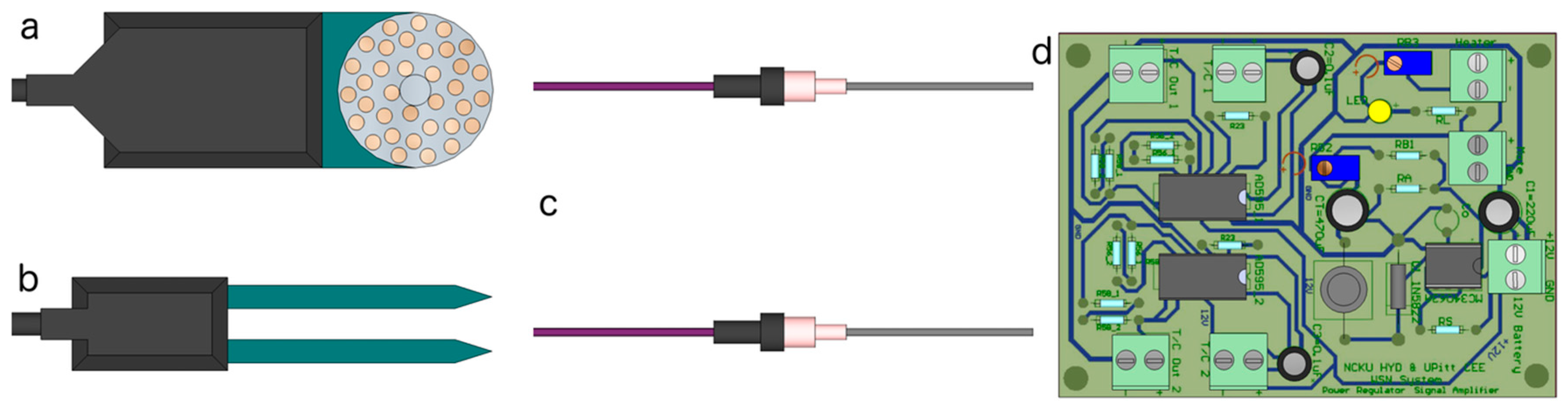
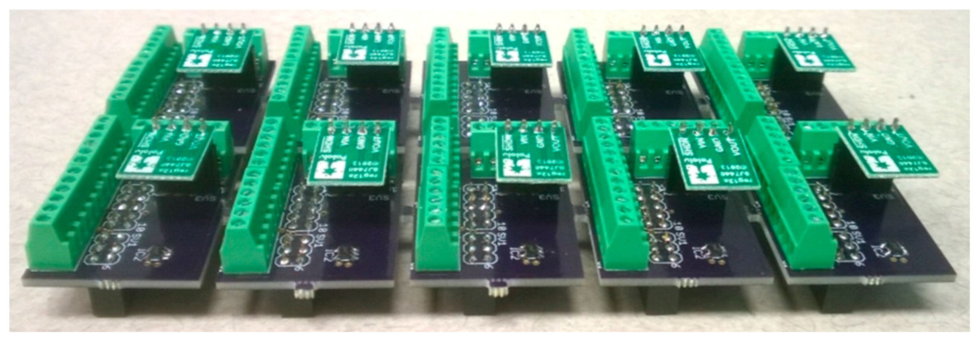
2.1.2. Updated Equipment (TelosB Motes and Custom Sensor Board)
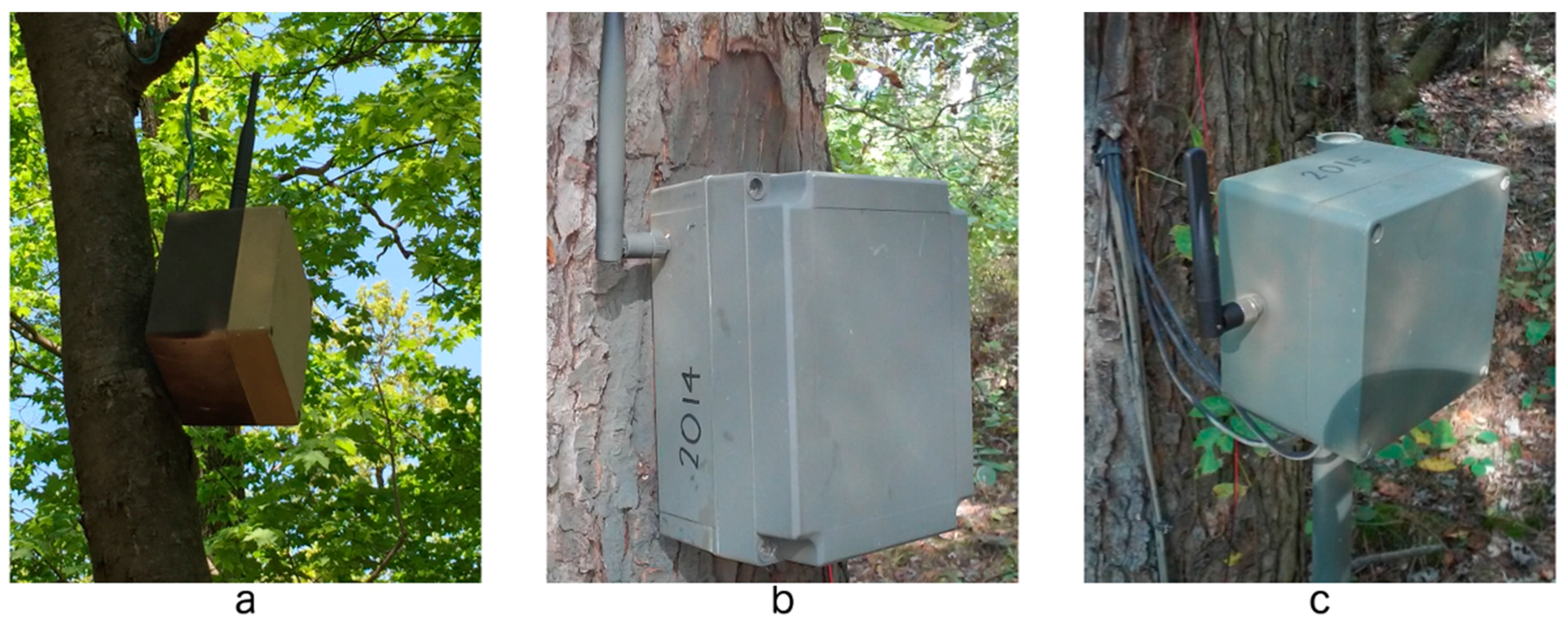
2.1.3. Enclosures
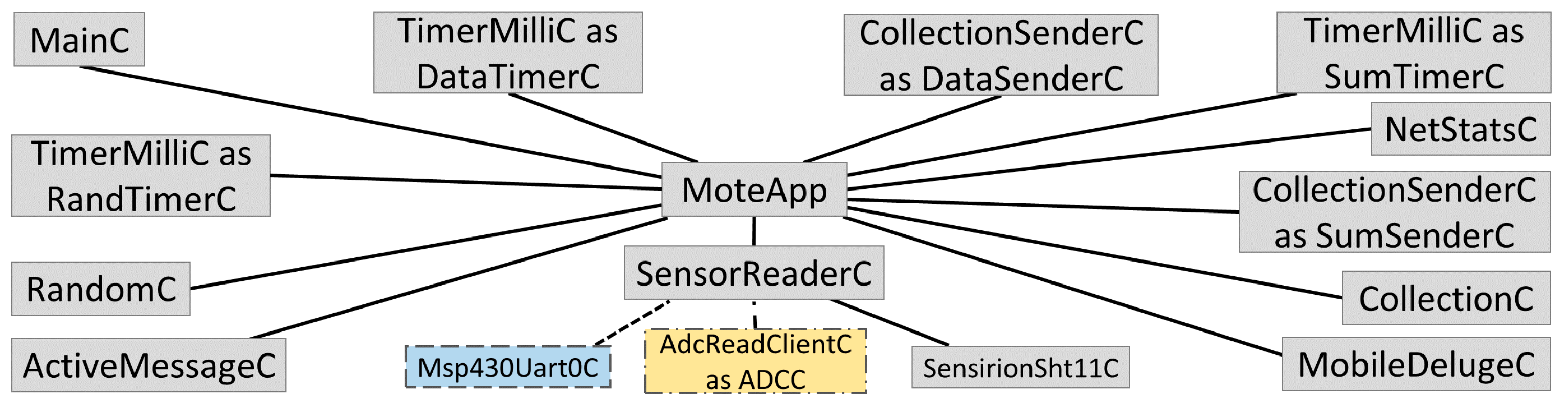
2.2. Mote Application
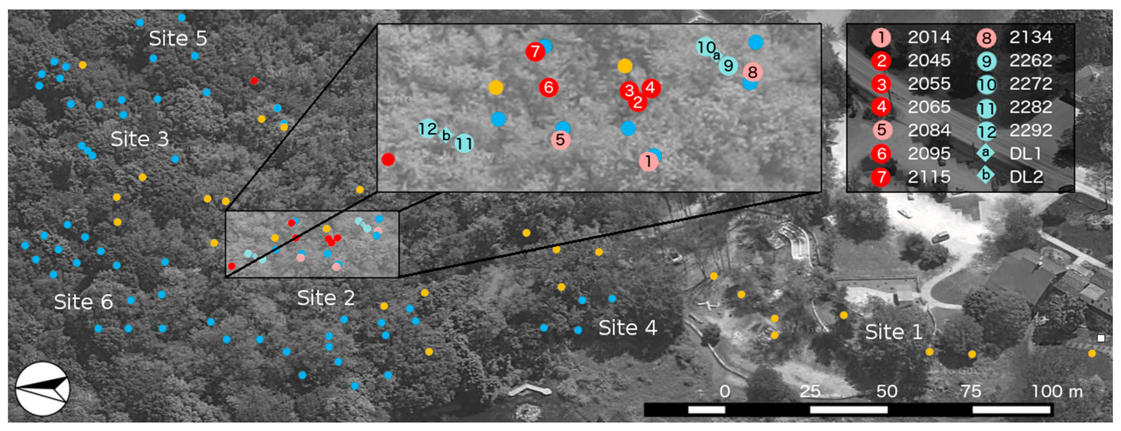
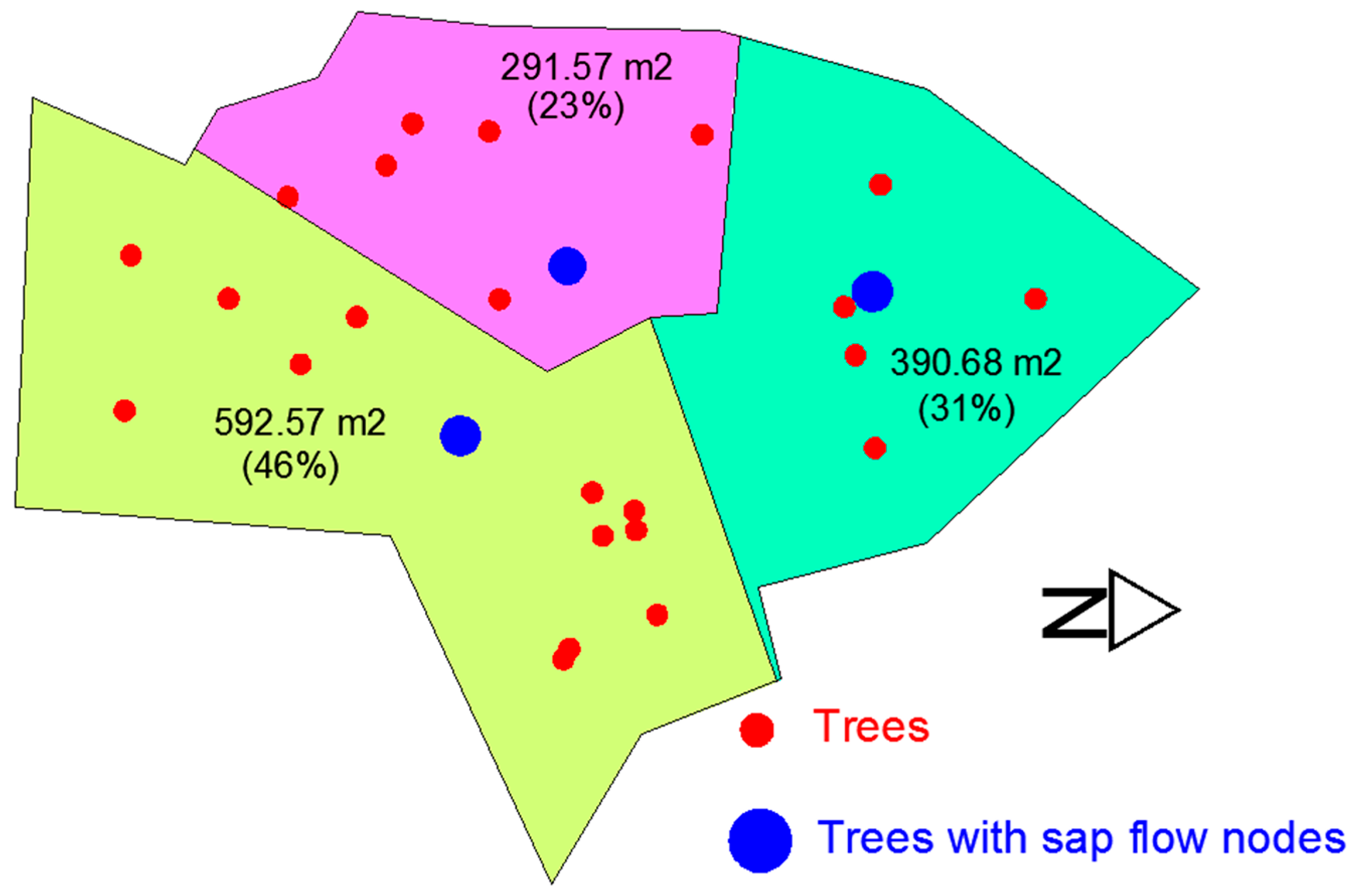
2.3. Deployment
2.4. Calibration of Soil Moisture Measurements
2.5. Hydraulic Properties from Soil Moisture Measurements
2.6. Transpiration Calculations from Sap Flow Measurements
2.7. Geostatistical Analysis of Soil Moisture and Soil Water Potential: Spatiotemporal Trends
3. Results and Discussion
3.1. Data Quality Assessment of WSN Sensors
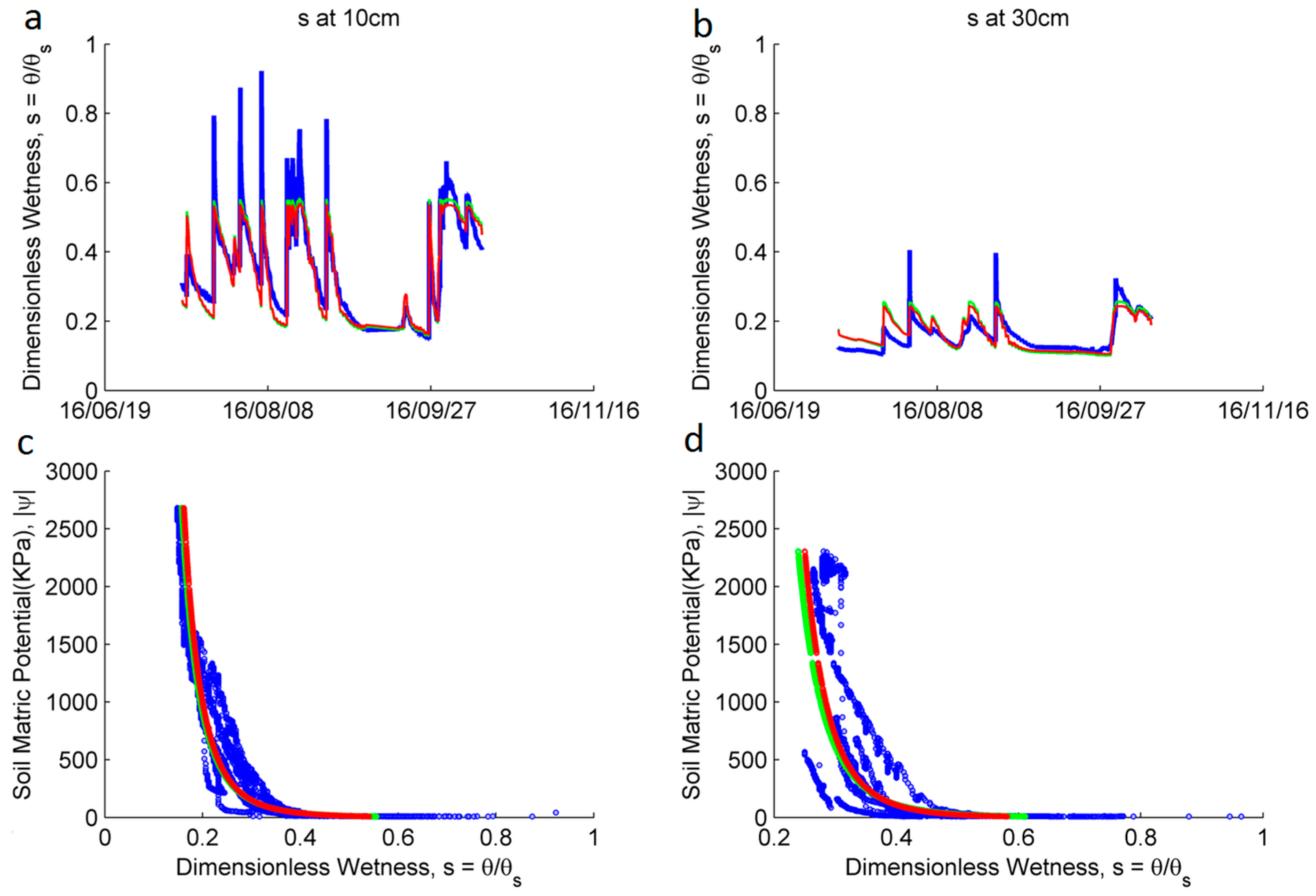
3.2. Hydraulic Properties Estimation
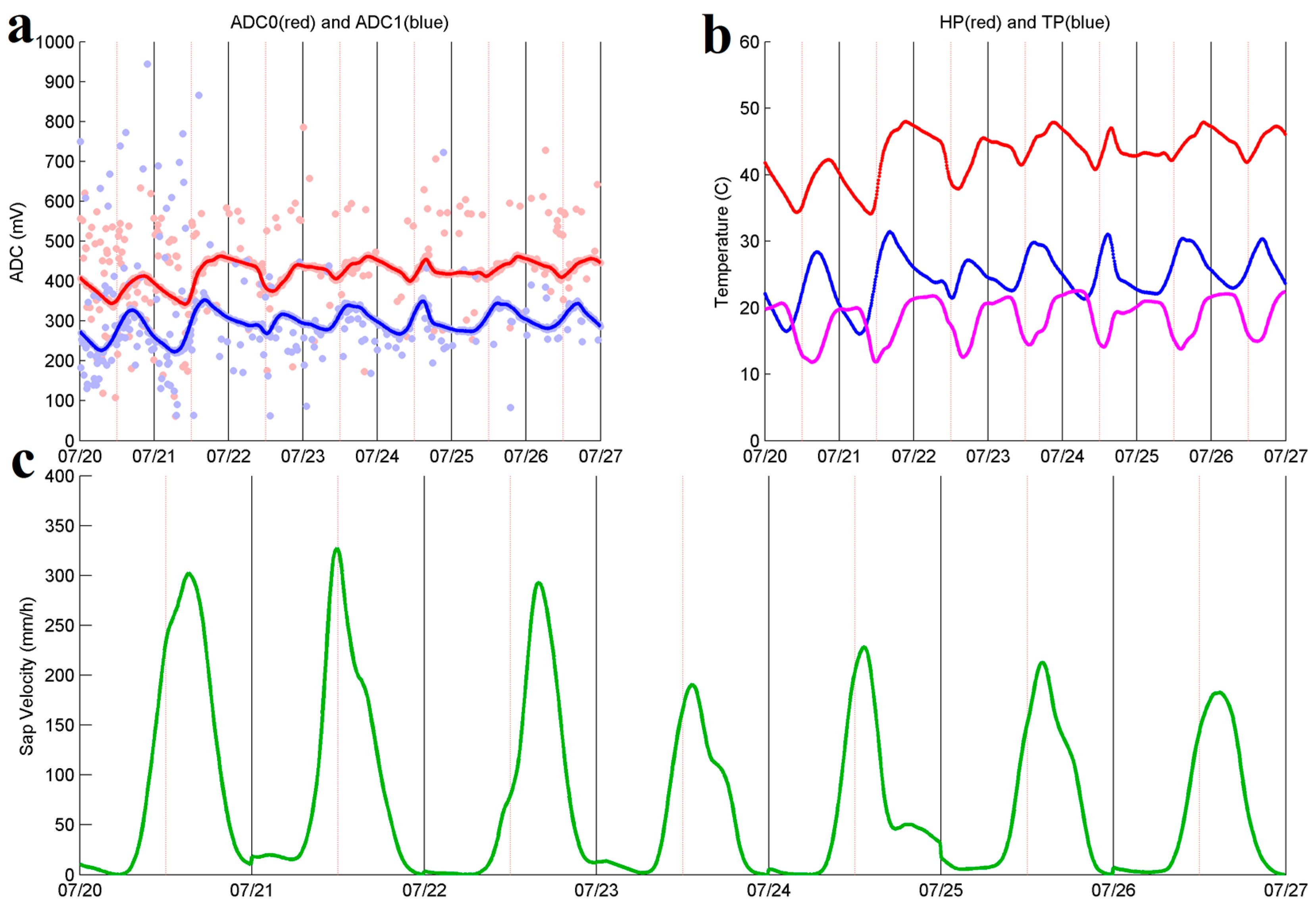
3.3. Sap Flow Data and Transpiration Estimation
3.3.1. Sap Flow Time Series
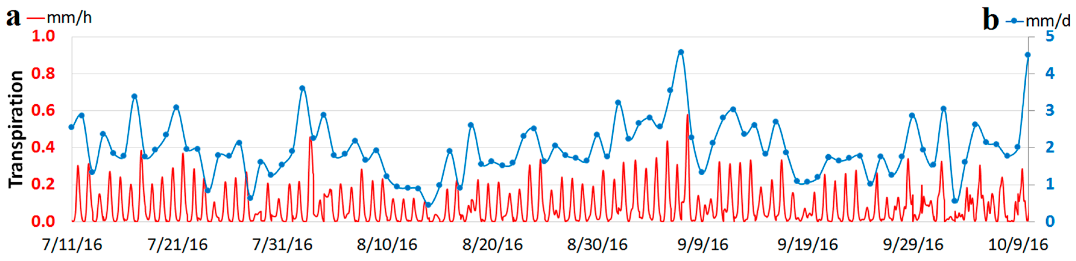
3.3.2. Transpiration Estimates from Sap Flow Measurements
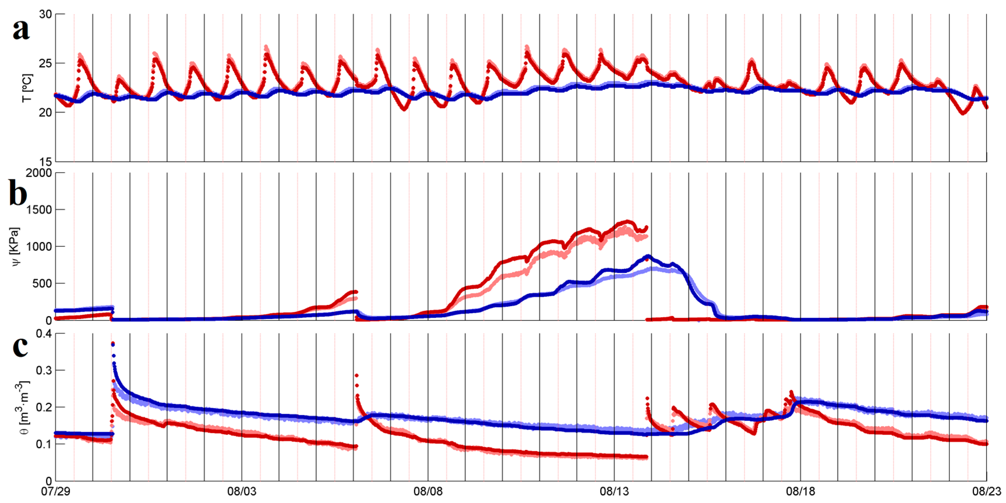
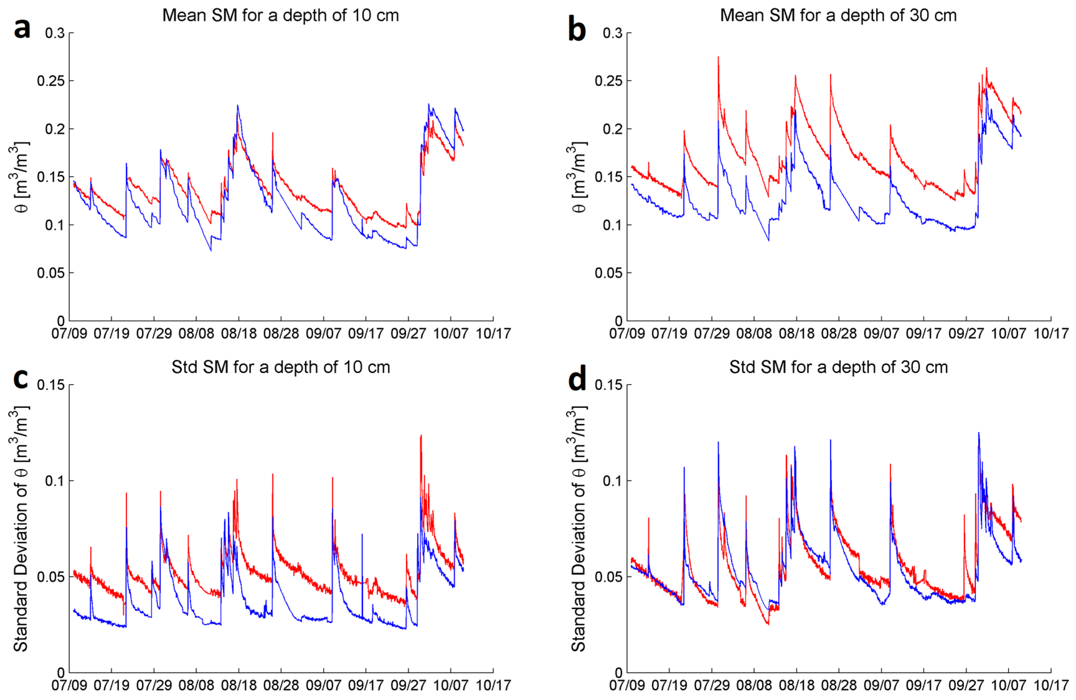
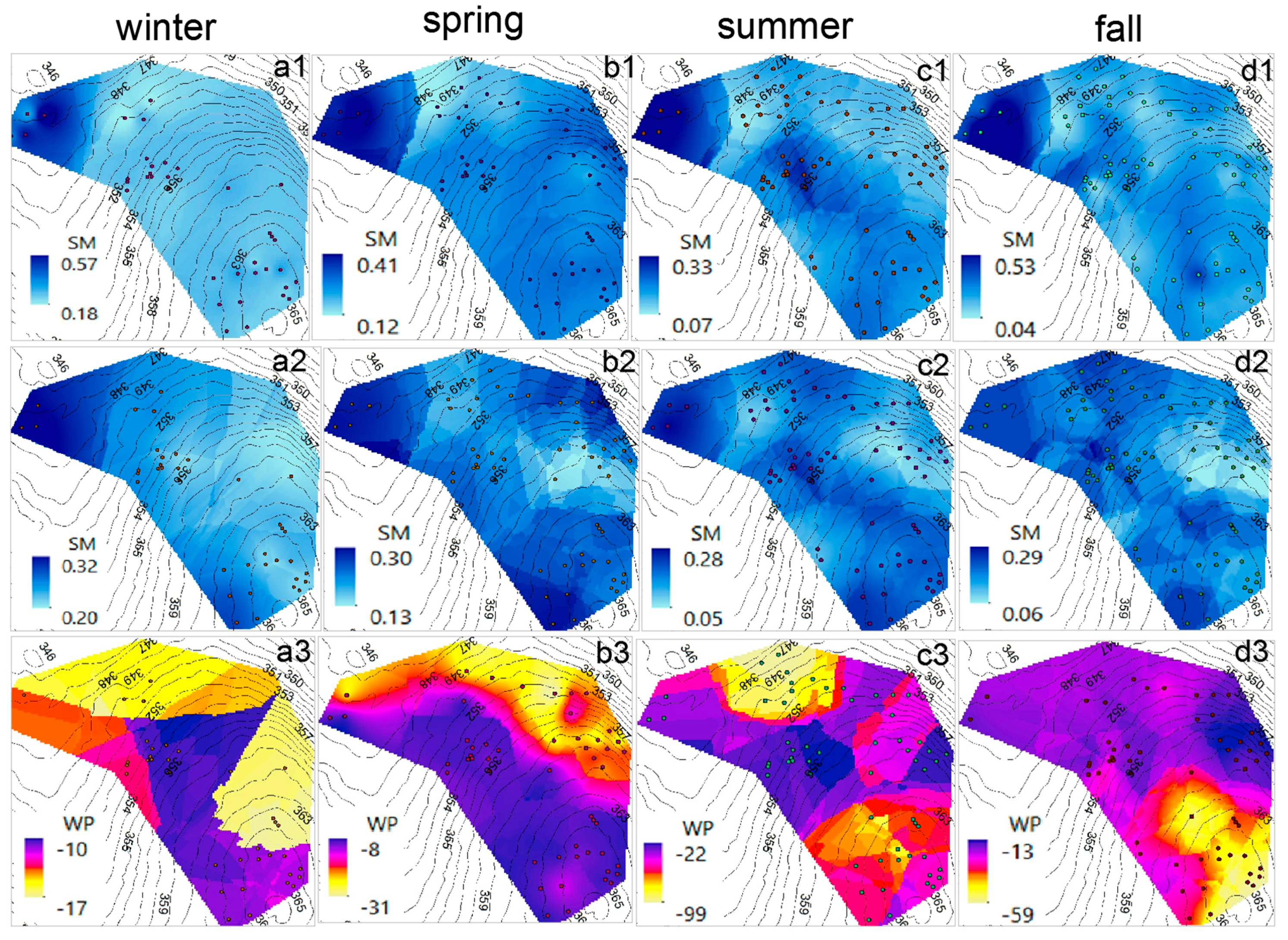
3.4. Exploration of Soil Moisture and Soil Water Potential: Spatiotemporal Trends
3.5. WSN Challenges and Utility in Hydrology
3.5.1. Power Management
3.5.2. Node Maintenance
3.5.3. Network Routing and Scaling
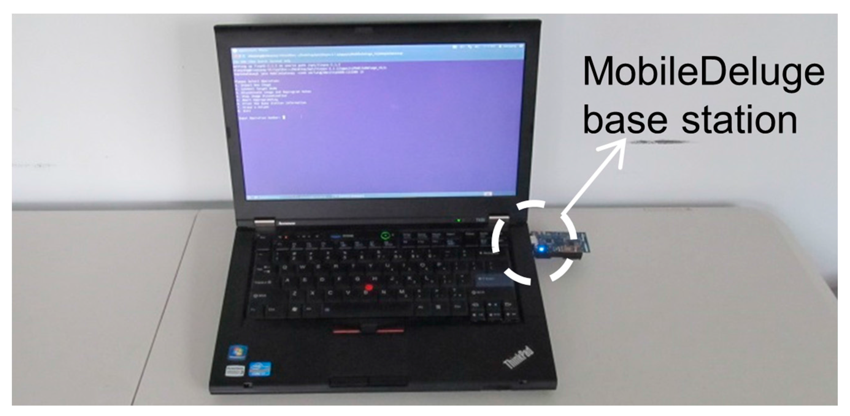
3.5.4. Heterogeneous Mote Reprogramming
3.5.5. Network Costs
3.6. Lessons Learned with Sap Flow
4. Conclusions
Acknowledgments
Author Contributions
Conflicts of Interest
References
- Holland, M.H.; Blood, E.R.; Shaffer, L.R. (Eds.) Achieving Sustainable Freshwater Systems: A Web of Connections; Island Press: Washington, DC, USA, 2003; p. 351.
- Beven, K. Changing ideas in hydrology—The case of physically-based models. J. Hydrol. 1989, 105, 157–172. [Google Scholar] [CrossRef]
- Oren, R.; Phillips, N.; Katul, G.; Ewers, B.E.; Pataki, D.E. Scaling xylem sap flux and soil water balance and calculating variance: A method for partitioning water flux in forests. Ann. For. Sci. 1998, 55, 191–216. [Google Scholar] [CrossRef]
- Ford, C.R.; Hubbard, R.M.; Kloeppel, B.D.; Vose, J.M. A comparison of sap flux-based evapotranspiration estimates with catchment-scale water balance. Agric. For. Meteorol. 2007, 145, 176–185. [Google Scholar] [CrossRef]
- Famiglietti, J.S.; Ryu, D.; Berg, A.A.; Rodell, M.; Jackson, T.J. Field observations of soil moisture variability across scales. Water Resour. Res. 2008, 44, W01423. [Google Scholar] [CrossRef]
- Akyildiz, I.F.; Su, W.; Sankarasubramaniam, Y.; Cayirci, E. Wireless sensor networks: A survey. Comput. Netw. 2002, 38, 393–422. [Google Scholar] [CrossRef]
- Rawat, P.; Singh, K.D.; Chaouchi, H.; Bonnin, J.M. Wireless sensor networks: A survey on recent developments and potential synergies. J. Supercomput. 2014, 68, 1–48. [Google Scholar] [CrossRef]
- Juang, P.; Oki, H.; Wang, Y.; Martonosi, M.; Peh, L.-S.; Rubenstein, D. Energy-efficient computing for wildlife tracking: Design tradeoffs and early experiences with ZebraNet. In Proceedings of the 10th International Conference on Architectural Support for Programming Languages and Operating Systems, San Jose, CA, USA, 5–9 October 2002.
- Mainwaring, A.; Culler, D.; Polastre, J.; Szewczyk, R.; Anderson, J. Wireless sensor networks for habitat monitoring. In Proceedings of the 1st ACM International Workshop on Wireless Sensor Networks and Applications, Atlanta, GA, USA, 28 September 2002.
- Szewczyk, R.; Polastre, J.; Mainwaring, A.; Culler, D. Lessons from a sensor network expedition. In Proceedings of the 1st European Workshop on Wireless Sensor Networks, Berlin, Germany, 19–21 January 2004.
- Tolle, A.; Polastre, J.; Szewczyk, R.; Culler, D.; Turner, N.; Tu, K.; Burgess, S.; Dawson, T.; Buonadonna, P.; Gay, D.; et al. A macroscope in the redwoods. In Proceedings of the 3rd International Conference on Embedded Networked Sensor Systems, San Diego, CA, USA, 2–4 November 2005.
- Hamilton, M.; Graham, E.A.; Rundel, P.W.; Allen, M.F.; Kaiser, W.; Hansen, M.L.; Estrin, D.L. New approaches in embedded networked sensing for terrestrial ecological observatories. Environ. Eng. Sci. 2007, 24, 192–204. [Google Scholar] [CrossRef]
- Werner-Allen, G.; Johnson, J.; Ruiz, M.; Lees, J.; Welsh, M. Monitoring volcanic eruptions with a wireless sensor network. In Proceedings of the Second European Workshop on Wireless Sensor Networks, Istanbul, Turkey, 2 February 2005.
- Werner-Allen, G.; Lorincz, K.; Welsh, M.; Marcillo, O.; Johnson, J.; Ruiz, M.; Lees, J. Deploying a wireless sensor network on an active volcano. IEEE Internet Comput. 2006, 10, 18–25. [Google Scholar] [CrossRef]
- Selavo, L.; Wood, A.; Cao, Q.; Sookoor, T.; Liu, H.; Srinivasan, A.; Wu, Y.; Kang, W.; Stankovic, J.; Young, D.; et al. LUSTER: Wireless sensor network for environmental research. In Proceedings of the 5th International Conference on Embedded Networked Sensor Systems, Sydney, Australia, 6–9 November 2007.
- Panchard, J.; Rao, S.; V, P.T.; Hubaux, J.-P.; Jamadagni, H.S. Commonsense net: A wireless sensor network for resource-poor agriculture in the semiarid areas of developing countries. Inf. Technol. Int. Dev. 2007, 4, 51–67. [Google Scholar] [CrossRef]
- Wark, T.; Corke, P.; Sikka, P.; Klingbeil, L.; Guo, Y.; Crossman, C.; Valencia, P.; Swain, D.; Bishop-Hurley, G. Transforming Agriculture through Pervasive Wireless Sensor Networks. IEEE Pervasive Comput. 2007, 6, 50–57. [Google Scholar] [CrossRef] [Green Version]
- Li, X.; Deng, Y.; Ding, L. Study on precision agriculture monitoring framework based on WSN. In Proceedings of the 2nd International Conference on Anti-Counterfeiting, Security and Identification, Guiyang, China, 20–23 August 2008.
- Martinelli, M.; Ioriatti, L.; Viani, F.; Benedetti, M.; Massa, A. A WSN-based solution for precision farm purposes. In Proceedings of the IEEE International Geoscience and Remote Sensing Symposium, Cape Town, South Africa, 12–17 July 2009.
- López, J.A.; Garcia-Sanchez, A.-J.; Soto, F.; Iborra, A.; Garcia-Sanchez, F.; Garcia-Haro, J. Design and validation of a wireless sensor network architecture for precision horticulture applications. Precis. Agric. 2011, 12, 280–295. [Google Scholar] [CrossRef]
- Viani, F. Experimental Validation of a wireless system for the irrigation management in smart farming applications. Microw. Opt. Technol. Lett. 2016, 58, 2186–2189. [Google Scholar] [CrossRef]
- Ferrández-Pastor, F.J.; Garcia-Chamizo, J.M.; Nieto-Hidalgo, M.; Mora-Pascual, J.; Mora-Martinez, J. Developing Ubiquitous Sensor Network Platform Using Internet of Things: Application in Precision Agriculture. Sensors 2016, 16, 1141. [Google Scholar] [CrossRef] [PubMed] [Green Version]
- Viani, F.; Bertolli, M.; Polo, A. Low-cost wireless system for agrochemical dosage reduction in precision farming. IEEE Sens. J. 2017, 17, 5–6. [Google Scholar] [CrossRef]
- López, J.A.; Soto, F.; Sánchez, P.; Iborra, A.; Suardiaz, J.; Vera, J.A. Development of a Sensor Node for Precision Horticulture. Sensors 2009, 9, 3240–3255. [Google Scholar] [CrossRef] [PubMed]
- Musăloiu-E, R.; Terzis, A.; Szlavecz, K.; Szalay, A.; Cogan, J.; Gray, J. Life under your feet: A wireless soil ecology sensor network. In Proceedings of the 3rd Workshop on Embedded Networked Sensors, Cambridge, UK, 30 May 2006.
- Suri, A.; Iyengar, S.S.; Cho, E. Ecoinformatics using wireless sensor networks: An overview. Ecol. Inform. 2006, 1, 287–293. [Google Scholar] [CrossRef]
- Rundel, P.W.; Graham, E.A.; Allen, M.F.; Fisher, J.C.; Harmon, T.C. Environmental sensor networks in ecological research. New Phytol. 2009, 182, 589–607. [Google Scholar] [CrossRef] [PubMed]
- Burgess, S.S.O.; Krantz, M.L.; Turner, N.E.; Cardell-Oliver, R.; Dawson, T.E. Harnessing wireless sensor technologies to advance forest ecology and agricultural research. Agric. For. Meteorol. 2010, 150, 30–37. [Google Scholar] [CrossRef]
- Trubilowicz, J.; Cai, K.; Weiler, M. Viability of motes for hydrological measurement. Water Resour. Res. 2009, 45, 1–6. [Google Scholar] [CrossRef]
- Ingelrest, F.; Barrenetxea, G.; Schaefer, G.; Vetterli, M.; Couach, O.; Parlange, M. SensorScope: Application-specific sensor network for environmental monitoring. ACM Trans. Sens. Netw. 2010, 6, 1–32. [Google Scholar] [CrossRef]
- Kerkez, B.; Glaser, S.D.; Bales, R.C.; Matthews, M.W. Design and performance of a wireless sensor network for catchment-scale snow and soil moisture measurements. Water Resour. Res. 2012, 48. [Google Scholar] [CrossRef]
- Navarro, M.; Davis, T.W.; Villalba, G.; Li, Y.; Zhong, X.; Erratt, N.; Liang, X.; Liang, Y. Towards long-term multi-hop WSN deployments for environmental monitoring: An experimental network evaluation. J. Sens. Actuator Netw. 2014, 4, 297–330. [Google Scholar] [CrossRef]
- Majone, B.; Viani, F.; Filippi, E.; Bellin, A.; Massa, A.; Toller, G.; Robol, F.; Salucci, M. Wireless sensor network deployment for monitoring soil moisture dynamics at the field scale. Procedia Environ. Sci. 2013, 19, 426–435. [Google Scholar] [CrossRef]
- Ryu, D.; Famiglietti, J.S. Characterization of footprint-scale surface soil moisture variability using Gaussian and beta distribution functions during the Southern Great Plains 1997 (SGP97) hydrology experiment. Water Resour. Res. 2005, 41. [Google Scholar] [CrossRef]
- Bogena, H.R.; Herbst, M.; Huisman, J.A.; Rosenbaum, U.; Weuthen, A.; Vereecken, H. Potential of Wireless Sensor Networks for Measuring Soil Water Content Variability. Vadose Zone J. 2010, 9, 1002–1013. [Google Scholar] [CrossRef]
- TinyOS. Available online: http://tinyos.net/ (accessed on 15 November 2016).
- Gnawali, O.; Fonseca, R.; Jamieson, K.; Kazandjieva, M.; Moss, D.; Levis, P. CTP: An efficient, robust, and reliable collection tree protocol for wireless sensor networks. ACM Trans. Sens. Netw. 2013, 10, 16. [Google Scholar] [CrossRef]
- Navarro, M.; Liang, Y. Efficient and Balanced Routing in Energy-Constrained Wireless Sensor Networks for Data Collection. In Proceedings of the 2016 International Conference on Embedded Wireless Systems and Networks (EWSN), Graz, Austria, 15–17 February 2016; pp. 101–113.
- Davis, T.W.; Kuo, C.-M.; Liang, X.; Yu, P.-S. Sap Flow Sensors: Construction, Quality Control and Comparison. Sensors 2012, 12, 954–971. [Google Scholar] [CrossRef] [PubMed]
- Granier, A. Une nouvelle méthode pour la mesure du flux de sève brute dans le tronc des arbres. Ann. Sci. For. 1985, 42, 193–200. [Google Scholar] [CrossRef]
- Granier, A. Evaluation of transpiration in a Douglas fir stand by means of sap flow measurements. Tree Physiol. 1987, 14, 179–190. [Google Scholar] [CrossRef]
- MPS-2 User Manual. Available online: http://manuals.decagon.com/Manuals/13755_MPS-2and6_Web.pdf (accessed on 13 March 2017).
- Davis, T.W.; Liang, X.; Kuo, C.-M.; Liang, Y. Analysis of Power Characteristics for Sap Flow, Soil Moisture, and Soil Water Potential Sensors in Wireless Sensor Networking Systems. IEEE Sens. J. 2012, 12, 1933–1945. [Google Scholar] [CrossRef]
- Llosa, J.; Vilajosana, I.; Vilajosana, X.; Navarro, N.; Surinach, E.; Marques, J.M. REMOTE, a wireless sensor network based system to monitor rowing performance. Sensors 2009, 9, 7069–7082. [Google Scholar] [CrossRef] [PubMed]
- Seto, E.Y.; Giani, A.; Shia, V.; Wang, C.; Yan, P.; Yang, A.Y.; Jerrett, M.; Bajcsy, R. A wireless body sensor network for the prevention and management of asthma. In Proceedings of the IEEE International Symposium on Industrial Embedded Systems (SIES’09), Lausanne, Switzerland, 8–10 July 2009; pp. 120–123.
- Kuryloski, P.; Giani, A.; Giannantonio, R.; Gilani, K.; Gravina, R.; Seppa, V.P.; Seto, E.; Shia, V.; Wang, C.; Yan, P.; et al. DexterNet: An open platform for heterogeneous body sensor networks and its applications. In Proceedings of the IEEE Sixth International Workshop on Wearable and Implantable Body Sensor Networks (BSN 2009), Berkeley, CA, USA, 3–5 June 2009; pp. 92–97.
- Cama, A.; Montoya, F.G.; Gómez, J.; De La Cruz, J.L.; Manzano-Agugliaro, F. Integration of communication technologies in sensor networks to monitor the Amazon environment. J. Clean. Prod. 2013, 59, 32–42. [Google Scholar] [CrossRef]
- Strazdins, G.; Elsts, A.; Nesenbergs, K.; Selavo, L. Wireless sensor network operating system design rules based on real-world deployment survey. J. Sens. Actuator Netw. 2013, 2, 509–556. [Google Scholar] [CrossRef]
- Amjad, M.; Sharif, M.; Afzal, M.K.; Kim, S.W. TinyOS-New Trends. Comparative Views, and Supported Sensing Applications: A Review. IEEE Sens. J. 2016, 16, 2865–2889. [Google Scholar] [CrossRef]
- Moss, D.; Levis, P. BoX-MACs: Exploiting Physical and Link Layer Boundaries in Low-Power Networking; Computer Systems Laboratory Stanford University: Stanford, CA, USA, 2008. [Google Scholar]
- Sensirion SHT11 Datasheet V5. Available online: https://www.sensirion.com/fileadmin/user_upload/customers/sensirion/Dokumente/2_Humidity_Sensors/Sensirion_Humidity_Sensors_SHT1x_Datasheet_V5.pdf (accessed on 13 March 2017).
- Zhong, X.; Navarro, M.; Villalba, G.; Liang, X.; Liang, Y. MobileDeluge: Mobile Code Dissemination for Wireless Sensor Networks. In Proceedings of the 2014 IEEE 11th International Conference on Mobile Ad Hoc and Sensor Systems, Philadelphia, PA, USA, 27–30 October 2014; pp. 363–370.
- Xu, Z.; Hu, T.; Song, Q. Bulk Data Dissemination in Low Power Sensor Networks: Present and Future Directions. Sensors 2017, 17, 156. [Google Scholar] [CrossRef] [PubMed]
- Cornelis, W.M.; Ronsyn, J.; van Meirvenne, M.; Hartmann, R. Evaluation of Pedotransfer Functions for Predicting the Soil Moisture Retention Curve. Soil Sci. Soc. Am. J. 2001, 65, 638. [Google Scholar] [CrossRef]
- Lin, H.; Zhang, W.; Yu, H. Hydropedology: Linking Dynamic Soil Properties with Soil Survey Data. In Application of Soil Physics in Environmental Analyses; Springer: Cham, Switzerland, 2014; pp. 23–50. [Google Scholar]
- Clapp, R.B.; Hornberger, G.M. Empirical equations for some soil hydraulic properties. Water Resour. Res. 1978, 14, 601–604. [Google Scholar] [CrossRef]
- Van Genuchten, M. A closed-form equation for predicting the hydraulic conductivity of unsaturated soils. Soil Sci. Soc. Am. J. 1980, 44, 892–898. [Google Scholar] [CrossRef]
- Edwards, W.; Becker, P.; Èermák, J. A unified nomenclature for sap flow measurements. Tree Physiol. 1996, 17, 65–67. [Google Scholar] [CrossRef]
- Granier, A.; Huc, R.; Barigah, S.T. Transpiration of natural rain forest and its dependence on climatic factors. Agric. For. Meteorol. 1996, 78, 19–29. [Google Scholar] [CrossRef]
- Wilson, K.B.; Hanson, P.J.; Mulholland, P.J.; Baldocchi, D.D.; Wullschleger, S.D. A comparison of methods for determining forest evapotranspiration and its components: Sap-flow, soil water budget, eddy covariance and catchment water balance. Agric. For. Meteorol. 2001, 106, 153–168. [Google Scholar] [CrossRef]
- Wullschleger, S.D. Transpiration from a multi-species deciduous forest as estimated by xylem sap flow techniques. For. Ecol. Manag. 2001, 143, 205–213. [Google Scholar] [CrossRef]
- Pataki, D.E.; Oren, R. Species differences in stomatal control of water loss at the canopy scale in a mature bottomland deciduous forest. Adv. Water Res. 2003, 26, 1267–1278. [Google Scholar] [CrossRef]
- Asbjornsen, H.; Tomer, M.D.; Gomez-Cardenas, M.; Brudvig, L.A.; Greenan, C.M.; Schilling, K. Tree and stand transpiration in a Midwestern bur oak savanna after elm encroachment and restoration thinning. For. Ecol. Manag. 2007, 247, 209–219. [Google Scholar] [CrossRef]
- Kumagai, T.; Aoki, S.; Nagasawa, H.; Mabuchi, T.; Kubota, K.; Inoue, S.; Utsumi, Y.; Otsuki, K. Effects of tree-to-tree and radial variations on sap flow estimates of transpiration in Japanese cedar. Agric. For. Meteorol. 2005, 135, 110–116. [Google Scholar] [CrossRef]
- Vertessy, R.A.; Benyon, S.K.; O’Sullivan, S.K.; Gribben, P.R. Relationships between stem diameter, sapwood area, leaf area, and transpiration in a young mountain ash forest. Tree Physiol. 1995, 15, 559–567. [Google Scholar] [CrossRef] [PubMed]
- Davis, T. Environmental Monitoring Through Wireless Sensor Networks. Ph.D. Thesis, University of Pittsburgh, Pittsburgh, PA, USA, 2012. [Google Scholar]
- Kang, J.; Jin, R.; Li, X. Regression kriging-based upscaling of soil moisture measurements from a wireless sensor network and multiresource remote sensing information over heterogeneous cropland. IEEE Lett. Geosci. Remote Sens. 2015, 12, 92–96. [Google Scholar] [CrossRef]
- Crow, W.T.; Berg, A.A.; Cosh, M.H.; Loew, A.; Mohanty, B.P.; Panciera, R.; deRosnay, P.; Ryu, D.; Walker, J.P. Upscaling sparse ground-based soil moisture observations for the validation of coarse-resolution satellite soil moisture products. Rev. Geophys. 2012, 50, RG2002. [Google Scholar] [CrossRef]
- Bosch, D.; Lakshmi, V.; Jackson, T.; Choi, M.; Jacobs, J. Large scale measurements of soil moisture for validation of remotely sensed data: Georgia soil moisture experiment of 2003. J. Hydrol. 2006, 323, 120–137. [Google Scholar] [CrossRef]
- Ford, T.W.; Quiring, S.M. Comparison and application of multiple methods for temporal interpolation of daily soil moisture. Int. J. Climatol. 2014, 34, 2604–2621. [Google Scholar] [CrossRef]
- Zhang, M.; Li, M.; Wang, W.; Liu, C.; Gao, H. Temporal and spatial variability of soil moisture based on WSN. Math. Comput. Model. 2013, 58, 826–833. [Google Scholar] [CrossRef]
- Zou, H.; Yue, Y.; Li, Q.; Yeh, A.G.O. An improved distance metric for the interpolation of link-based traffic data using kriging: A case study of a large-scale urban road network. Int. J. Geogr. Inf. Sci. 2012, 26, 667–689. [Google Scholar] [CrossRef]
- Zhang, J.; Chen, H.; Su, Y.; Shi, Y.; Zhang, W.; Kong, X. Spatial Variability of Surface Soil Moisture in a Depression Area of Karst Region. Clean Soil Air Water 2011, 39, 619–625. [Google Scholar] [CrossRef]
- Lyon, S.W.; Sorensen, R.; Stendahl, J.; Seibert, J. Using landscape characteristics to define an adjusted distance metric for improving kriging interpolations. Int. J. Geogr. Inf. Sci. 2010, 24, 723–740. [Google Scholar] [CrossRef] [Green Version]
- Lakhankar, T.; Jones, A.S.; Combs, C.L.; Sengupta, M.; Vonder Haar, T.H.; Khanbilvardi, R. Analysis of Large Scale Spatial Variability of Soil Moisture Using a Geostatistical Method. Sensors 2010, 10, 913–932. [Google Scholar] [CrossRef] [PubMed]
- Ali, A.; Ikpehai, A.; Adebisi, B.; Mihaylova, L. Location prediction optimisation in WSNs using Kriging interpolation. IET Wirel. Sens. Syst. 2016, 6, 74–81. [Google Scholar] [CrossRef] [Green Version]
- Oliver, M.; Webster, R. A tutorial guide to geostatistics: Computing and modelling variograms and kriging. Catena 2014, 113, 56–69. [Google Scholar] [CrossRef]
- Konak, A. Estimating path loss in wireless local area networks using ordinary kriging. In Proceedings of the 2010 Winter Simulation Conference, Baltimore, MD, USA, 5–8 December 2010; pp. 2888–2896.
- Umer, M.; Kulik, L.; Tanin, E. Spatial interpolation in wireless sensor networks: Localized algorithms for variogram modeling and kriging. Geoinformatica 2010, 14, 101–134. [Google Scholar] [CrossRef]
- Camilli, A.; Cugnasca, C.E.; Saraiva, A.M.; Hirakawa, A.R.; Corrêa, P.L.P. From wireless sensors to field mapping: Anatomy of an application for precision agriculture. Comput. Electron. Agric. 2007, 58, 25–36. [Google Scholar] [CrossRef]
- Bardossy, A.; Lehmann, W. Spatial distribution of soil moisture in a small catchment. Part 1: Geostatistical analysis. J. Hydrol. 1998, 206, 1–15. [Google Scholar] [CrossRef]
- Teegavarapu, R.S.V.; Chandramouli, V. Improved weighting methods, deterministic and stochastic data-driven models for estimation of missing precipitation records. J. Hydrol. 2005, 312, 191–206. [Google Scholar]
- Vicente-Serrano, S.M.; Sanchez, S.; Cuadrat, J.M. Comparative analysis of interpolation methods in the middle Ebro Valley (Spain): Application to annual precipitation and temperature. Clim. Res. 2003, 24, 161–180. [Google Scholar] [CrossRef]
- Goovaerts, P. Geostatistical approaches for incorporating elevation into the spatial interpolation of rainfall. J. Hydrol. 2000, 228, 113–129. [Google Scholar] [CrossRef]
- Nash, J.E.; Sutcliffe, J.V. River flow forecasting through conceptual models. Part I—A discussion of principles. J. Hydrol. 1970, 10, 282–290. [Google Scholar] [CrossRef]
- Cleveland, W.S. Robust Locally Weighted Regression and Smoothing Scatterplots. J. Am. Stat. Assoc. 1979, 74, 829–836. [Google Scholar] [CrossRef]
- Northeast Regional Climate Center (NRCC). Available online: http://www.nrcc.cornell.edu (accessed on 15 November 2016).
- Tromp-van Meerveld, H.J.; McDonnell, J.J. On the interrelations between topography, soil depth, soil moisture, transpiration rates and species distribution at the hillslope scale. Adv. Water Resour. 2006, 29, 293–310. [Google Scholar] [CrossRef]
- Domec, J.-C.; Sun, G.; Noormets, A.; Gavazzi, M.J.; Treasure, E.A.; Cohen, E.; Swenson, J.J.; McNulty, S.G.; King, J.S. A Comparison of Three Methods to Estimate Evapotranspiration in Two Contrasting Loblolly Pine Plantations: Age-Related Changes in Water Use and Drought Sensitivity of Evapotranspiration Components. For. Sci. 2012, 58, 497–512. [Google Scholar] [CrossRef]
- Chang, N.-B. Multiscale Hydrologic Remote Sensing: Perspectives and Applications; Taylor & Francis: Boca Raton, FL, USA, 2012. [Google Scholar]
- Pittsburgh Airport Meteorological Station. Available online: http://www.usclimatedata.com/climate/pittsburgh/pennsylvania/united-states/uspa3601 (accessed on 15 November 2016).
- Thierfelder, T.K.; Grayson, R.B.; von Rosena, D.; Western, A.W. Inferring the location of catchment characteristic soil moisture monitoring sites: Covariance structures in the temporal domain. J. Hydrol. 2003, 280, 13–32. [Google Scholar] [CrossRef]
- Oliveira, L.M.; Rodrigues, J.J. Wireless Sensor Networks: A Survey on Environmental Monitoring. J. Commun. 2011, 6. [Google Scholar] [CrossRef]
- Davis, T.W.; Liang, X.; Navarro, M.; Bhatnagar, D.; Liang, Y. An Experimental Study of WSN Power Efficiency: MICAz Networks with XMesh. Int. J. Distrib. Sens. Netw. 2012, 2012, 1–14. [Google Scholar] [CrossRef]
- Navarro, M.; Li, Y.; Liang, Y. Energy profile for environmental monitoring wireless sensor networks. In Proceedings of the 2014 IEEE Colombian Conference on Communications and Computing (COLCOM), Bogota, Colombia, 4–6 June 2014; pp. 1–6.
- Beutel, J.; Romer, K.; Ringwald, M.; Woehrle, M. Deployment techniques for sensor networks. In Sensor Networks: Where Theory Meets Practice; Ferrari, G., Ed.; Springer: Berlin, Germany, 2010; pp. 219–248. [Google Scholar]
- Navarro, M.; Bhatnagar, D.; Liang, Y. An integrated network and data management system for heterogeneous WSNs. In Proceedings of the IEEE MASS 2011, Wuhan, China, 12–14 August 2011; pp. 819–824.
- Ringgaard, R.; Herbst, M.; Friborg, T. Partitioning of forest evapotranspiration: The impact of edge effects and canopy structure. Agric. For. Meteorol. 2012, 166, 86–97. [Google Scholar] [CrossRef]
- Hui, J.W.; Culler, D. The dynamic behavior of a data dissemination protocol for network programming at scale. In Proceedings of the 2nd International Conference on Embedded Networked Sensor Systems—SenSys’04; ACM Press: New York, NY, USA, 2004; p. 81. [Google Scholar]
- Burgess, S.O.; Dawson, T.E. Using branch and basal trunk sap flow measurements to estimate whole-plant water capacitance: A caution. Plant Soil 2008, 305, 5–13. [Google Scholar] [CrossRef]


| Location | Depth (cm) | θs | b | ψs (kPa) | NSE (Clapp-Hornberger) | n | α | NSE (Van Genuchten) |
|---|---|---|---|---|---|---|---|---|
| DL1 | 10 | 0.32 | 9.63 | 0.045 | 0.914 | 1.093 | 62.34 | 0.929 |
| DL1 | 30 | 0.44 | 10.69 | 0.00066 | 0.800 | 1.081 | 10814.0 | 0.821 |
| DL2 | 10 | 0.31 | 4.49 | 0.658 | 0.921 | 1.215 | 1.808 | 0.922 |
| DL2 | 30 | 0.42 | 5.87 | 0.521 | 0.801 | 1.154 | 3.51 | 0.812 |
| Node | (cm) a | (%) b | (cm2) c | (cm2) d | (cm2) e |
|---|---|---|---|---|---|
| 2045 | 34 | 77.4 | 839 | 650 | 700 |
| 2055 | 30.7 | 70 | 682 | 478 | 601 |
| 2065 | 31.5 | 76.7 | 719 | 552 | 633 |
| 2095 | 41.2 | 81.7 | 1250 | 1020 | 954 |
| 2115 | 24.3 | 83.1 | 415 | 345 | 394 |
| Survey Regions | (m2) a | (ha) b | (m2/ha) |
|---|---|---|---|
| 2134 | 0.375 | 0.0292 | 12.87 |
| 2084 | 0.38 | 0.0391 | 9.73 |
| 2014 | 0.784 | 0.0593 | 13.23 |
| Interpolated Surface | SM (m3·m−3) at 10 cm | SM (m3·m−3) at 30 cm | WP (kPa) at 30 cm | |||||||||
|---|---|---|---|---|---|---|---|---|---|---|---|---|
| # Nodes | Max SM | Min SM | RMSE | # Nodes | Max SM | Min SM | RMSE | # Nodes | Max WP | Min WP | RMSE | |
| Winter 2010–2016 | 38 | 0.570 | 0.180 | 0.061 | 38 | 0.320 | 0.200 | 0.030 | 37 | −10 | −17 | 2.12 |
| Spring 2010–2016 | 55 | 0.410 | 0.120 | 0.062 | 57 | 0.300 | 0.130 | 0.048 | 51 | −8 | −31 | 4.94 |
| Summer 2010–2016 | 71 | 0.330 | 0.070 | 0.061 | 72 | 0.280 | 0.050 | 0.052 | 59 | −22 | −99 | 17.46 |
| Fall 2010–2016 | 72 | 0.530 | 0.040 | 0.063 | 72 | 0.290 | 0.060 | 0.051 | 57 | −13 | −59 | 6.01 |
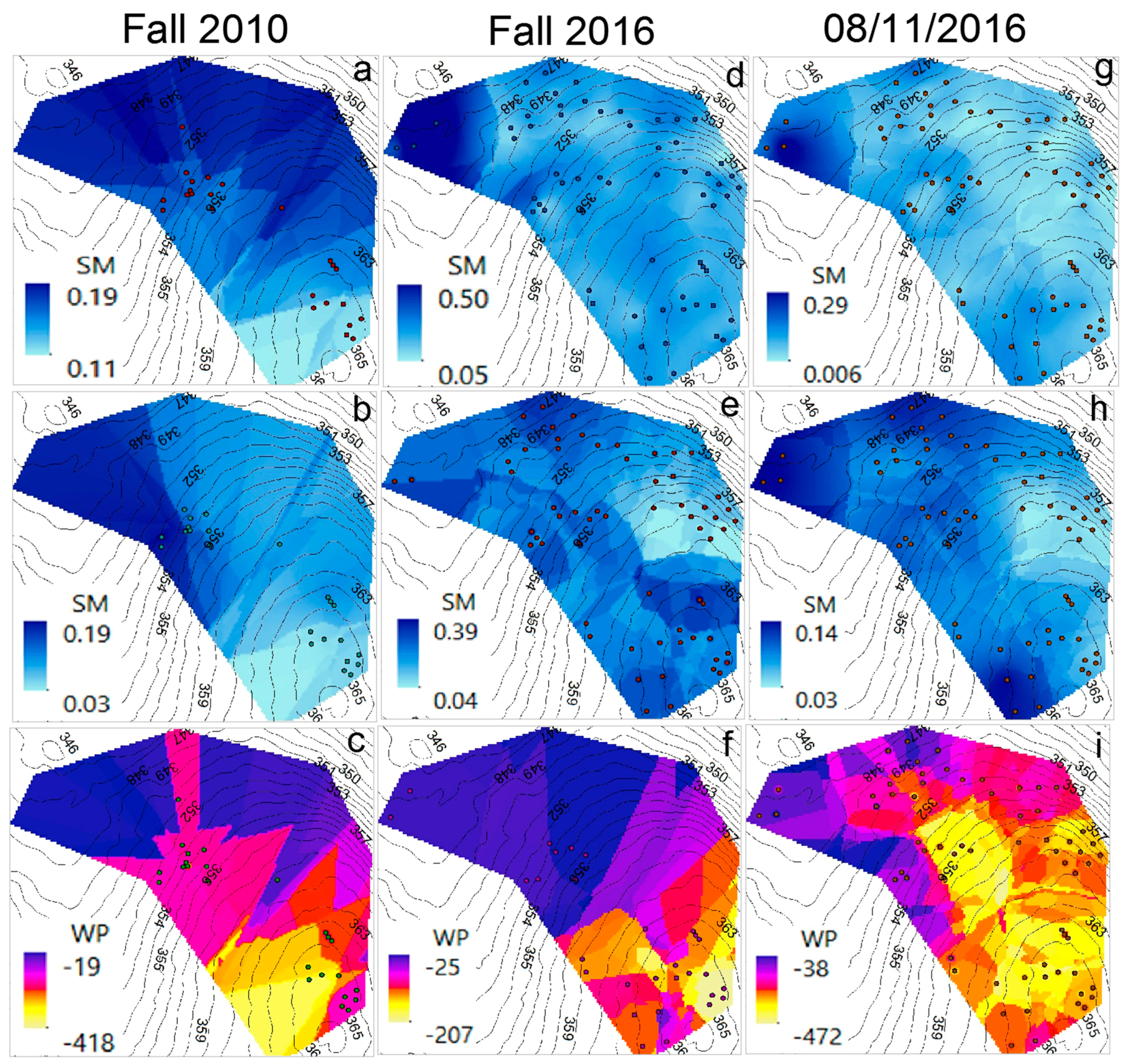
| Fall 2010 | 24 | 0.190 | 0.110 | 0.059 | 23 | 0.190 | 0.030 | 0.058 | 24 | −19 | −418 | 41.91 |
| Fall 2016 | 72 | 0.500 | 0.050 | 0.026 | 72 | 0.390 | 0.040 | 0.057 | 69 | −25 | −207 | 17.88 |
| 8/11/2016 | 74 | 0.290 | 0.006 | 0.031 | 74 | 0.140 | 0.030 | 0.024 | 74 | −38 | −472 | 26.53 |
| App Type | Number |
|---|---|
| Relays | 27 |
| Soil Moisture Water Potential (EC-5 × 2, MPS-1 × 1) | 31 |
| Soil Moisture Water Potential (EC-5 × 2, MPS-2 × 1) | 36 |
| Sap Flow | 10 |
© 2017 by the authors. Licensee MDPI, Basel, Switzerland. This article is an open access article distributed under the terms and conditions of the Creative Commons Attribution (CC BY) license ( http://creativecommons.org/licenses/by/4.0/).
Share and Cite
Villalba, G.; Plaza, F.; Zhong, X.; Davis, T.W.; Navarro, M.; Li, Y.; Slater, T.A.; Liang, Y.; Liang, X. A Networked Sensor System for the Analysis of Plot-Scale Hydrology. Sensors 2017, 17, 636. https://doi.org/10.3390/s17030636
Villalba G, Plaza F, Zhong X, Davis TW, Navarro M, Li Y, Slater TA, Liang Y, Liang X. A Networked Sensor System for the Analysis of Plot-Scale Hydrology. Sensors. 2017; 17(3):636. https://doi.org/10.3390/s17030636
Chicago/Turabian StyleVillalba, German, Fernando Plaza, Xiaoyang Zhong, Tyler W. Davis, Miguel Navarro, Yimei Li, Thomas A. Slater, Yao Liang, and Xu Liang. 2017. "A Networked Sensor System for the Analysis of Plot-Scale Hydrology" Sensors 17, no. 3: 636. https://doi.org/10.3390/s17030636