
Indoor Autonomous Control of a Two-Wheeled Inverted Pendulum Vehicle Using Ultra Wide Band Technology

Key Laboratory of Micro-inertial Instrument and Advanced Navigation Technology, Ministry of Education, School of Instrument Science and Engineering, Southeast University, Nanjing 210096, China
*
Author to whom correspondence should be addressed.
Sensors 2017, 17(6), 1401; https://doi.org/10.3390/s17061401
Submission received: 6 March 2017
/
Revised: 10 May 2017
/
Accepted: 10 May 2017
/
Published: 15 June 2017
(This article belongs to the Collection Modeling, Testing and Reliability Issues in MEMS Engineering)
Abstract
:In this paper, we aimed to achieve the indoor tracking control of a two-wheeled inverted pendulum (TWIP) vehicle. The attitude data are acquired from a low cost micro inertial measurement unit (IMU), and the ultra-wideband (UWB) technology is utilized to obtain an accurate estimation of the TWIP’s position. We propose a dual-loop control method to realize the simultaneous balance and trajectory tracking control for the TWIP vehicle. A robust adaptive second-order sliding mode control (2-RASMC) method based on an improved super-twisting (STW) algorithm is investigated to obtain the control laws, followed by several simulations to verify its robustness. The outer loop controller is designed using the idea of backstepping. Moreover, three typical trajectories, including a circle, a trifolium and a hexagon, have been designed to prove the adaptability of the control combinations. Six different combinations of inner and outer loop control algorithms have been compared, and the characteristics of inner and outer loop algorithm combinations have been analyzed. Simulation results demonstrate its tracking performance and thus verify the validity of the proposed control methods. Trajectory tracking experiments in a real indoor environment have been performed using our experimental vehicle to further validate the feasibility of the proposed algorithm in practice.
1. Introduction
Two-wheeled inverted pendulum (TWIP) vehicles are a popular test platform to validate the performance of advanced control algorithms, such as the control capacity for nonlinear, instability and rapidity situations. The motion of a TWIP vehicle is governed by its under-actuated configuration, which makes it difficult to control by simply applying traditional robotics approaches [1]. In recent years, control design for the stability and robustness of TWIP vehicles has attracted great research interest. In [2], a neural network control method was proposed for an under-actuated wheeled inverted pendulum model with small overshoot and quick response to changes in the desired trajectories. In [3], adaptive backstepping control for a two-wheeled autonomous robot around an operating point was investigated. In [4], an adaptation concept was brought into neural network control, which demonstrated the yaw angle and pitch angle convergence time was less than 0.4 s with an initial value of 0.3 rad.
The sliding mode control (SMC) method was first proposed by Soviet scholars in the 1960s. The SMC method has some advantages such as robustness to parameter uncertainty, insensitivity to bounded disturbances, fast dynamic response, a remarkable computational simplicity with respect to other robust control approaches, and easy implementation of the controller [5,6]. However, the chattering caused by the discontinuous sliding controller more or less limits its application in practice [7].
The high-order sliding mode control (HOSMC) method is the further improvement of the traditional sliding mode control, yielding less chattering and better convergence accuracy while preserving its robustness properties [8,9]. Consequently, HOSMC methods have been actively investigated in recent years for chattering attenuation and robust control of unknown uncertainties and perturbations, respectively. Levant put forward the 2-SMC method based on a differentiation and output-feedback control system in [10], and there are many different 2-SMC algorithms that have been presented such as the ‘twisting’ and ‘super-twisting’ ones put forward by Levant, the ‘sub-optimal’ and ‘global’ ones developed by Bartolini and so on.
The objective of this paper is to sustain the self-balance and trajectory tracking of a TWIP vehicle in a GPS denied environment. Nakano et al. have proposed an estimation/control structure in a two-wheeled vehicle where both a camera and a target object are attached to the vehicle [11]. The major drawback of the approach based on camera is that it may produce a heavy computational load and lead to a low real-time performance. Accuracy and precision are the two main performance parameters of the indoor localization system. Portable UWB radio ranging technology was introduced in [12,13]. The UWB local positioning system can be used as a standalone system or as a complementary system where the GPS is unavailable or denied, can meet high real-time requirements and even penetrate through objects (such as walls, obstacles, bodies, etc.) to a certain extent.
In this paper, a prototype TWIP vehicle (shown in Figure 1) was built in our lab. The TWIP vehicle consists of two independent drive wheels on the same axle, two rotary encoders, a car body and other auxiliary devices such as a sensor (MPU-6050) which has an embedded 3-axis MEMS gyroscope, a 3-axis MEMS accelerometer (MEMS sensors have the advantages of miniaturization and high-performance [14]) and a portable I-UWB locating tag.
The control system configuration of our testbed is illustrated in Figure 2. The attitude data of the TWIP vehicle is measured via the onboard IMU, the location information of the TWIP vehicle is measured by an onboard UWB receiver and used to control the motion of the vehicle. In Figure 2, A0, A1, A2 and A3 are four UWB positioning technology anchors, T0 is a UWB receiver used as an onboard tag. The TWIP vehicle can communicate with both cellphones and laptops via Bluetooth devices.
This paper is organized as follows: in Section 2, the nonlinear dynamic model of the TWIP vehicle is established using a Lagrange energy equation. In Section 3, inner and outer loop controllers are designed, and necessary stability considerations are discussed. Then the feasibility and effectiveness of the different control methods are compared by MATLAB simulation in Section 4, followed by the conclusions in Section 5. The configuration of an experimental set-up of the TWIP vehicle and the results are given in Section 6.
2. Related Work
A second-order adaptive sliding mode control method based on STW algorithm was proposed for the control of an under-actuated system in [15], which performed better effectiveness and reduced chattering compared with conventional SMC and ordinary second-order SMC. However, the adaptive sliding mode control method is not very effective for a controller of multi-control parameters. In [16], the structure of the inner/outer loop control system has been used in simultaneous balancing and trajectory tracking control for two-wheeled inverted pendulum vehicles, and two trajectories, including a circle and a trifolium have been designed for tracking. For the purpose of controlling the TWIP vehicle, an inner/outer loop control structure and a second-order STW algorithm have been also used in this paper. We proposed a different adaptive control method in this paper to keep convergence of sliding mode surface under unknown disturbances. What’s more, three typical trajectories, including a circle, a trifolium and a hexagon, have been designed to prove the adaptability of our controller.
3. System Description and Modeling
The motion of the TWIP vehicle is described under an inertial coordinate system. The simplified schematic diagram and the two-dimensional plan view of the vehicle are shown in Figure 3.
The origin O of the fixed coordinate system OXY is the center of the axle, the positive direction of OX-axis is the forward motion of TWIP, OY-axis is coincident with the axle, the positive direction of OZ-axis is vertically upward. The parameters and variables of the system are shown in Table 1. During the motion process of our two-wheeled vehicle, since there are only two points contacting with the ground, and the body has a motion similar to inverted pendulum motion, we can make a few assumptions in order to build dynamic model for the system:
- (1)
- There exists sufficient friction between the wheels and the ground, which makes the system subject to non-holonomic constraints, i.e., the assumption of no sliding and skidding holds throughout.
- (2)
- Take the TWIP vehicle as a perfectly rigid body, the distance from the center of mass of the body to the axle is ;
- (3)
- The influence caused by the dynamic characteristics of DC motors is ignored;
- (4)
- Ignore the effects caused by friction and damping force of bearings and revolute pairs to the motion state of the system.
In the paper, we adopt the Lagrange energy equation to build the kinematic model of the two-wheeled car. In order to eliminate the effect caused by the non-holonomic constraint, we choose as the generalized coordinates system, then the kinematic model of the two-wheeled car can be written in the following form:
where, denotes the inertia matrix, is the vector of coriolis and centrifugal forces is the vector of gravitational forces, denotes the matrix of control coefficients, is the vector of control inputs.
Defining a new velocity vector , then the relationship between a new coordinate vector and the generalized coordinate vector can be written as follows:
Then the dynamics of the system can be formulated as follows:
where:
In order to simplify the controller design, the state-space equations can be derived from (3):
where:
is known as the system state. is the system control input, and , .
4. Design of the Controller
An inner/outer loop controller needs to be designed to make the vehicle achieve trajectory tracking on the ground while maintaining its own balance. The structure of the designed inner/outer loop control system is shown in Figure 4. The inner loop control consists of two control subsystems: the rotational velocity control subsystem and the longitudinal velocity and balance control subsystem. , are defined as the desired value of the longitudinal velocity v and the rotational velocity ω respectively. And the tracking errors of v and ω are introduced as , . A reference trajectory is known in prior as , , , and the control laws of and are given by the outer loop controller.
4.1. Inner Loop Controller Design
Considering the desired inclination angle = 0, a set of error state-space equations can be obtained as follows:
4.1.1. The Rotational Velocity Control
It is well known that the classical discontinuous sliding mode control provides finite-time convergence for a system of relative degree one. As the rotational velocity control subsystem (7) has a relative degree equal to two, a sliding surface is needed when using STW algorithm.
The tracking error of δ is introduced as . And the equilibrium point of system (7) can be defined as . Defining a traditional linear sliding surface as:
where, is a positive constant. Differentiating (10) with respect to time, it follows that:
where, .
The continuous control law is constituted by two terms. The first is defined by means of its discontinuous time derivative, while the other is a continuous function of the available sliding surface .
Assume that there exists a bounded time-variable disturbance signal in the system (7), which satisfies , L is a Lipschitz constant. According to the STW algorithm [10], the control law of can be obtained as follows:
Theorem 1.
According to the convergent method proposed in [17], when , , the states of system (7) can reach in finite time, and converge to origin.
4.1.2. The Longitudinal Velocity and Balance Control
We define , as the expected values of longitudinal displacement and longitudinal velocity v respectively and consider the tracking errors of , as , . The equilibrium point of systems (8) and (9) can be defined as . The control law of is designed to make the vehicle accomplish the ultimate objective, that is, when t → ∞, as well as .
Due to its ingenious design, simple algorithm structure and good control effect, hierarchical sliding mode control theory is widely used in complex under-actuated systems control [18,19,20]. Therefore, we adopt the hierarchical sliding mode surface to design the control law of .
In order to design control strategy, two traditional linear sliding mode surfaces with known positive constants c2 and c3 are defined as:
Differentiating s2 and s3 with respect to time, we can obtain:
A control law based on piecewise linear hierarchical sliding mode control method needs to be changed occasionally, bringing in severe oscillation during the control process. In view of the decoupled sliding-mode control method introduced in [21], a hierarchical sliding mode control method based on model analysis is proposed.
The first layer sliding mode surface s2 and s3 is used to construct the second layer sliding mode surface S. Define the second layer sliding mode surface S as:
Differentiating (15) with respect to time and then:
where and are Lipschitz continuous.
Assume that there exists a bounded time-variable disturbance signal in the systems (8) and (9), which satisfies , is a Lipschitz constant. Similar to the analysis of rotational angle control, the 2-SMC control law for the longitudinal velocity and balance control subsystems (8) and (9) can be deduced as follows:
where, S is the sliding mode surface of the control subsystem.
Theorem 2.
According to Theorem 1, when , the states of subsystems (8) and (9) can reach and converge to origin in finite time with the control law (17).
Proof.
The process to prove the subsystems (8) and (9) can reach is similar to Theorem 1’s, so for simplicity, the proof is omitted here. Suppose that at a moment before the system return back to the equilibrium position. A negative control input is given to push to zero, that is,. At this moment, under the same negative control input, and . Since α is chosen as a positive constant, when S converges to 0, and can always satisfy the condition that , , and gradually converge to 0 and vice versa. It can be concluded that subsystems (8) and (9) will converge to in exponential form. ☐
4.1.3. Robust Adaptive 2-SMC (2-RASMC)
Considering the rotational velocity control subsystem (7), when are unknown functions, defining a new coordinate vector , the system model can be written as the following form:
where is assumed strict positivity without loss of generality, and are bounded unknown functions, and satisfying the following inequalities with positive constants :
As the system model contains uncertain part, the control input can be designed as two parts:
where, is the nominal part of , and is the compensation control part of .
The nominal system model ( can be obtained as:
According to Theorem 2, the control system (22) is asymptotically stable and reach within finite time with the following control law of :
In view of an adaptive sliding mode control method introduced in [19], an adaptive sliding mode control law of is proposed, with which the system perturbation can be compensated. Firstly, an auxiliary variable is introduced and satisfying , then define a sliding mode variable as:
Differentiating (24) with respect to time, it is easily obtained that:
where, is the total uncertainty of the system, and satisfying , where is an unknown positive constant. Let us consider as the estimation of true value , and consequently an estimated error can be governed by . In addition, considering the fact that is exhibiting slow time-varying behaviors, then, it holds that .
The compensation control law for the subsystem can be given by:
with the adaptive law as follows:
Theorem 3.
Consider the given dynamic sliding mode (24) with the nominal controller (23) and the compensation controller(26), the sliding mode variable σ = 0 can be guaranteed in finite time.
Proof.
Consider a positive Lyapunov candidate as:
By differentiating V with respect to time and considering , it holds that:
It can be seen that for . By LaSalle's invariance principle [22,23] and the Lyapunov stability criterion [24], the theorem is proved.
Similar to the above analysis, we can deduce the robust adaptive 2-SMC control law for the longitudinal velocity and balance control subsystems (8) and (9) as follows:
where, S is the sliding mode surface (15) of the control subsystem. ☐
Theorem 4.
According to Theorems 2 and 3, when , the state of systems (8) and (9) can reach with the control law (31), and converge to origin in finite time. The proof process is similar with above and is omitted here.
4.1.4. Comparative Simulations for the Robust Performance
In this section, a comparative simulation has been done to verify the robustness of the modified 2-RASMC control method. Since the 2-RASMC controller is based on the 2-SMC controller, they share the same control parameters, except two additional parameters and . We have done a lot of simulations to find the appropriate control parameters of the designed controller.
Set rad/s, m/s as the control target for the 2-RASMC controller. Then the initial state variables are supposed as .
Figure 5 depicts the control performance of our controller for tracking the descried and with six different sets of designed parameters as Table 2 shows. Figure 5 shows the control performance of case1~case6 without system uncertainty. It can be concluded that the controllers have the same control performance when the control parameters of the nominal controllers are the same. It can be easily obtained that case 1 and case 2 have the best control performance.
During the process of tuning the control parameters, we have found the effects of the controller parameters on control performance. The increases of , , , , and contribute to the faster convergence speed, and make overshoot volume increase. However, the increase of contributes to bigger overshoot volume and longer settling time of θ, and bigger overshoot volume and shorter settling time of v. The increase of makes overshoot volume of θ decrease, overshoot volume of v increase, and slows down the convergence speed of θ and v.
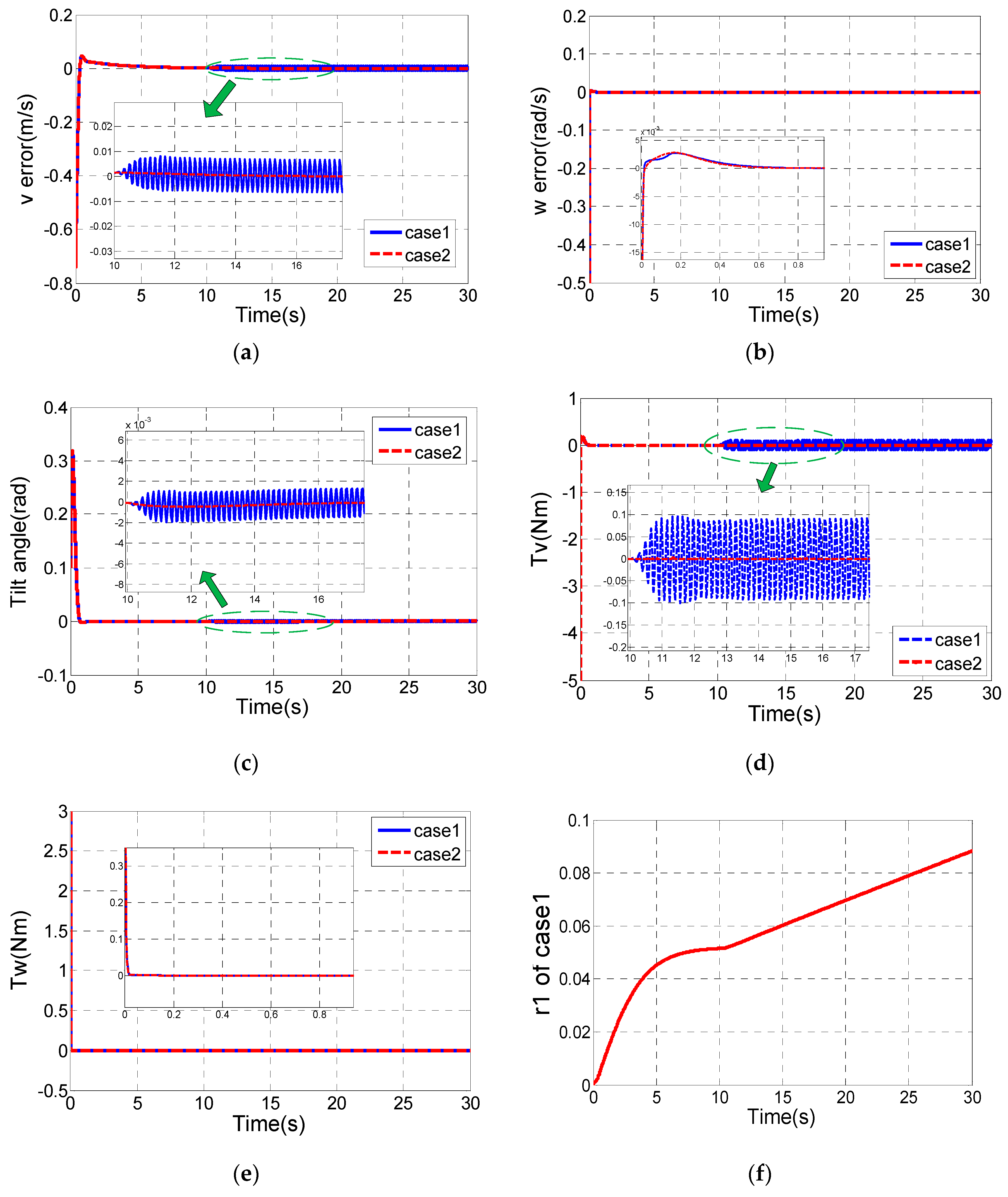
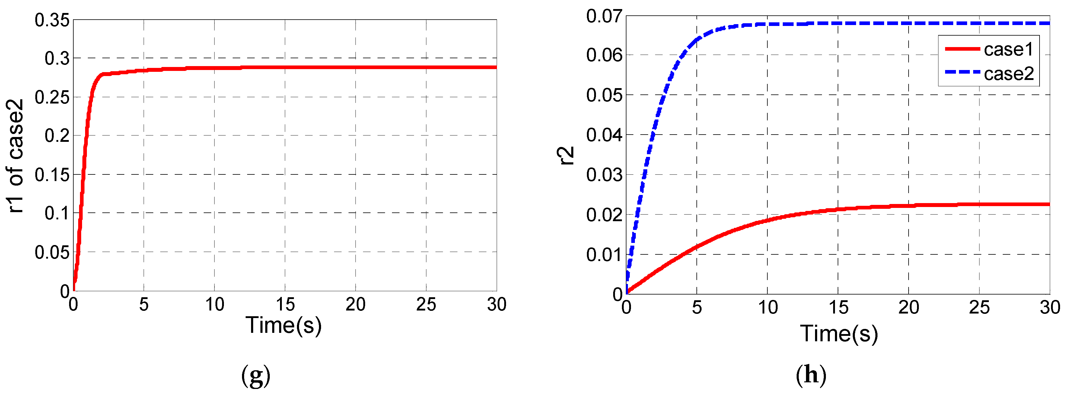
Then we will consider the control performance of case1 and case2 with system uncertainty. We assumed that the mass of the body is considered as a variable value in the simulation:
Figure 6 shows the simulation results of case1 and case2.
It can be seen that case2 has better robustness than case1, so we choose the same control parameters as case2. The designed parameters of the inner loop controller are shown in Table 3.
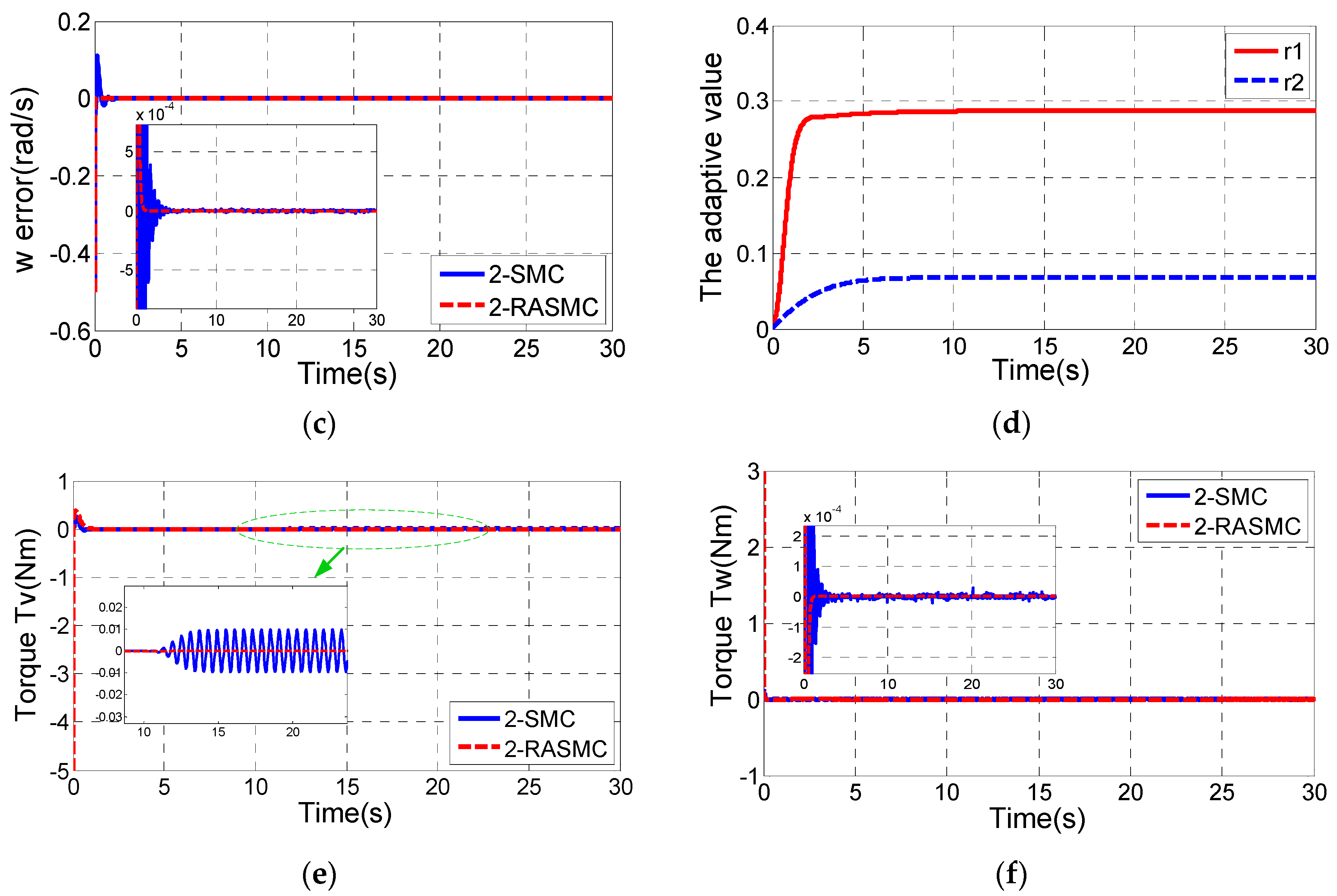
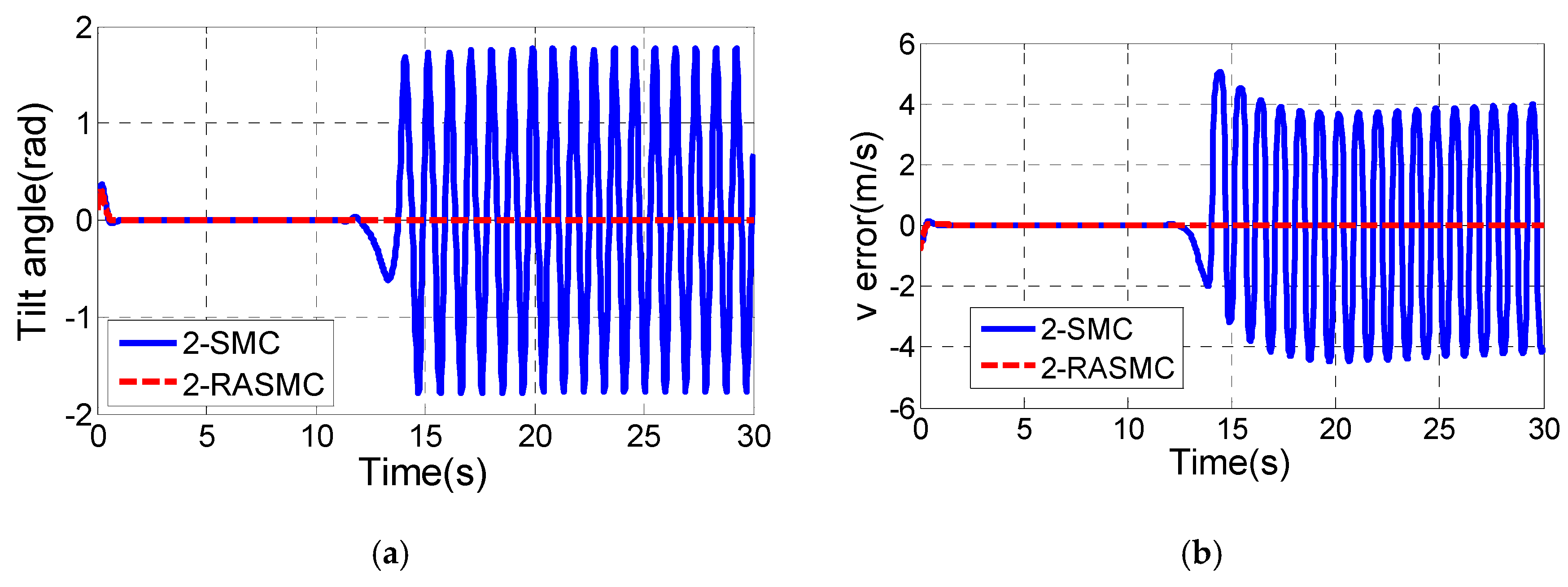
Set rad/s, m/s as the control target for our inner loop controller. Then the initial state variables are supposed as . In order to verify the robustness of the two controllers, the mass of the body is considered as a variable value in the simulation:
Figure 7 shows the simulation results.
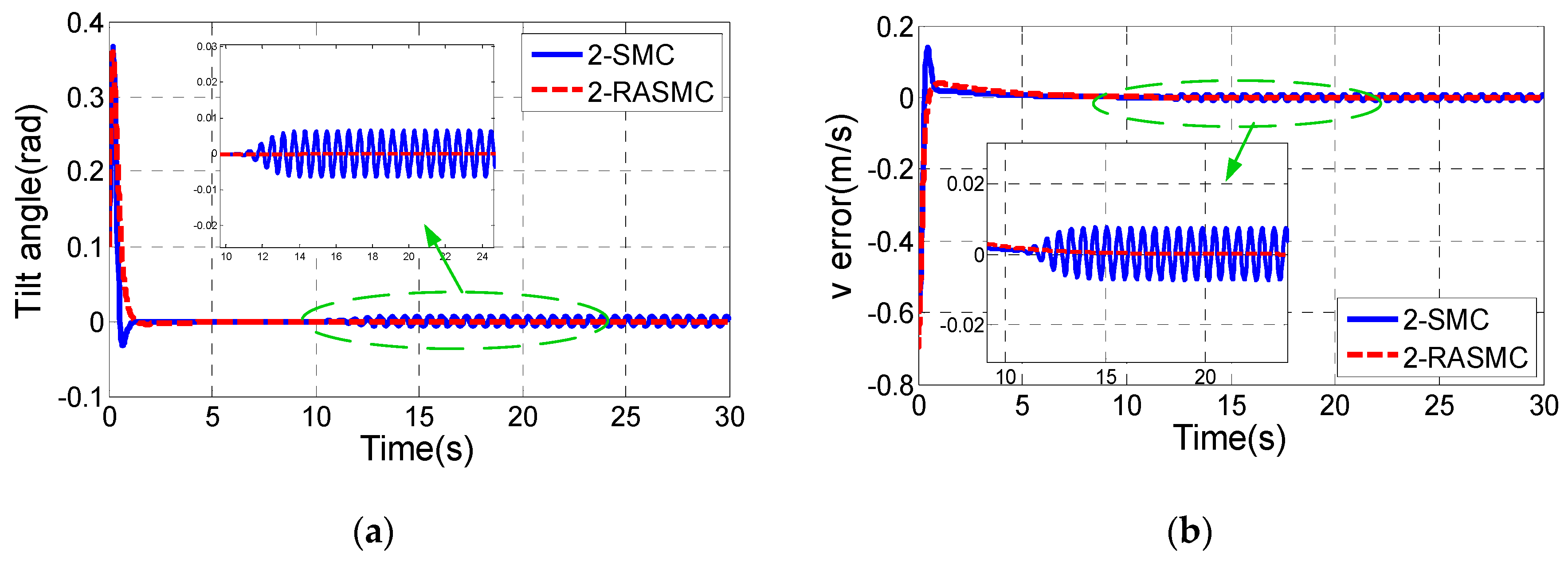
Comparing Figure 7a,b,e with Figure 7c,f, it can be concluded that the robust performance of the control law of ω is much better than that of the control law of v in the 2-SMC controller. Considering Figure 7a,b,e, it can be easily seen that the state variables of the subsystems (8) and (9) in the 2-SMC controller oscillates near the equilibrium point after t > 10 s, while the control performance of the 2-RASMC controller is almost unaffected.
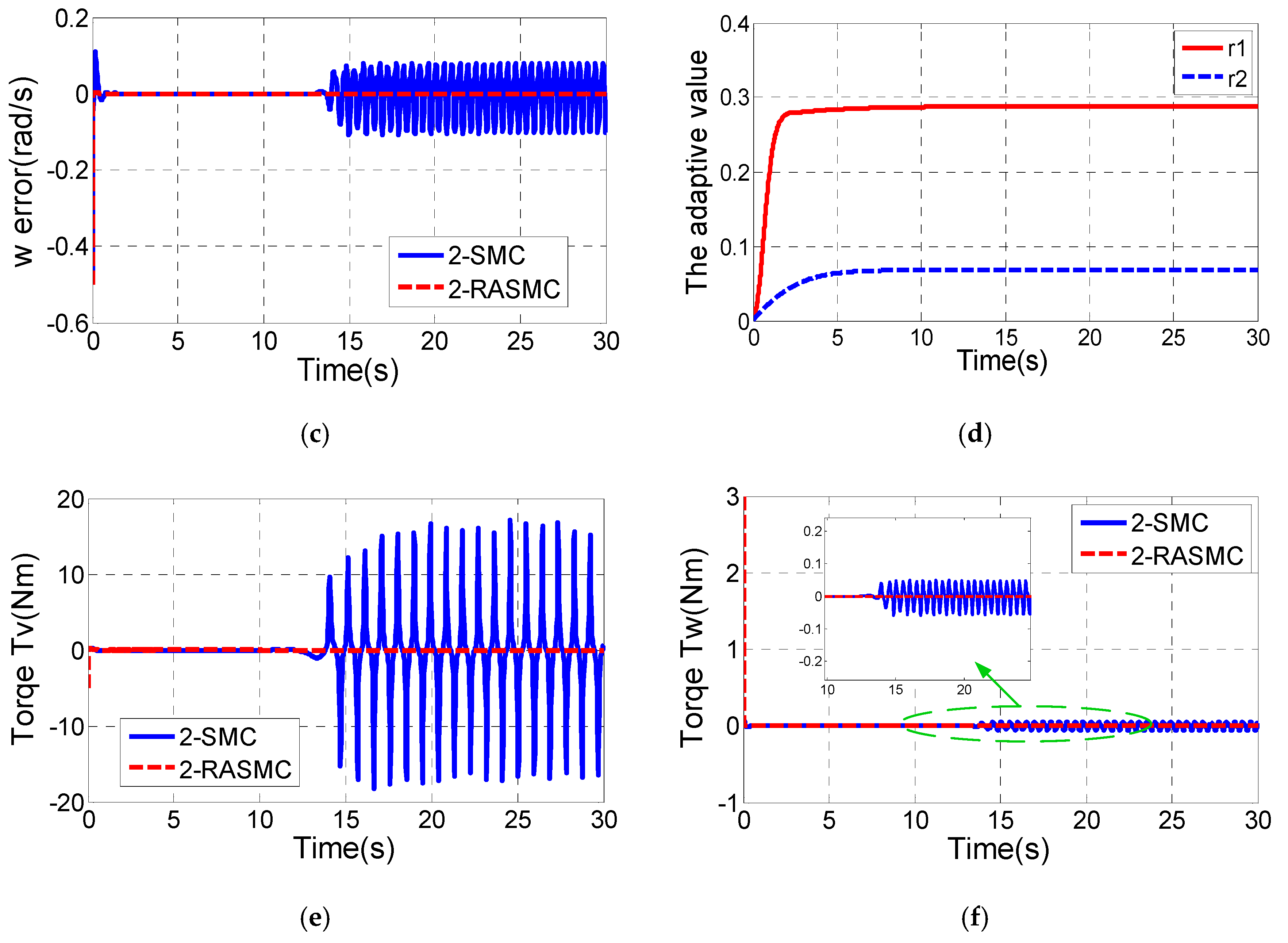
By increasing the value of m, the comparison of the robust performance of the two controllers will be more obvious. Set the value of m as , then the simulation result is shown as Figure 8.
From Figure 8, we can see the control performance of the 2-SMC controller becomes terrible after t > 10 s, while the 2-RASMC controller still maintains good control performance although the degree of system uncertainty is exacerbated. Combining Figure 7 and Figure 8, it can be observed that the 2-RASMC controller has better robustness.
4.2. Outer Loop Controller Design
The motion states of the TWIP vehicle on x-y plane are described by the center position of its wheel axis O (x, y) and the heading angle δ as shown in Figure 9. Defining , , the kinematic equations of the vehicle can be obtained as:
Defining as the reference trajectory in the earth fixed coordinate system, then the reference longitudinal and rotational velocities can be calculated in prior respectively. The position and orientation errors are defined as:
Differentiating (33) with respect to time, the tracking error dynamics can be obtained as:
Backstepping control method is often used to deal with underactuated stabilization. Backstepping has good tracking performance, fast response time without overshoot and is suitable for online control. Therefore, we design the outer-loop controller using the idea of backstepping.
Take as a virtual control variable, the new error variable is defined as:
When and , according to Equation (35):
Lemma 1.
For all , and the absolute value of x is bounded, there is , if and only if x = 0 the equality holds.
So, when t→ ∞, ye exponentially converges to zero, thus xe→0.
Adopting backstepping control method, the control law is deduced as follows:
where, λ1, λ2, λ3 and λ4 are the designed positive constants.
Theorem 5.
The control system (34) is stable, and the posture errors are asymptotically stable with the backstepping control law (37).
Proof.
First, define a Lyapunov candidate as:
Differentiating Equation (38) with respect to time:
Substituting the control law equations of ω and v (37) into Equation (39), then:
5. Simulation and Discussion
In this section, a lot of comparative simulations have been done to verify the validity of the proposed control methods. We have done a lot of simulations and found the appropriate control parameters of the designed outer loop controller as shown in Table 4. Table 5 exhibits several different algorithmic approaches combined by diverse control methods of inner and outer loop controllers. The simulation framework for 2S-B controller is shown in Figure A1 of the Appendix.
The control parameters of the PID controller used for comparison in this paper are settled by the Ziegler-Nichols method and shown in Table 6.
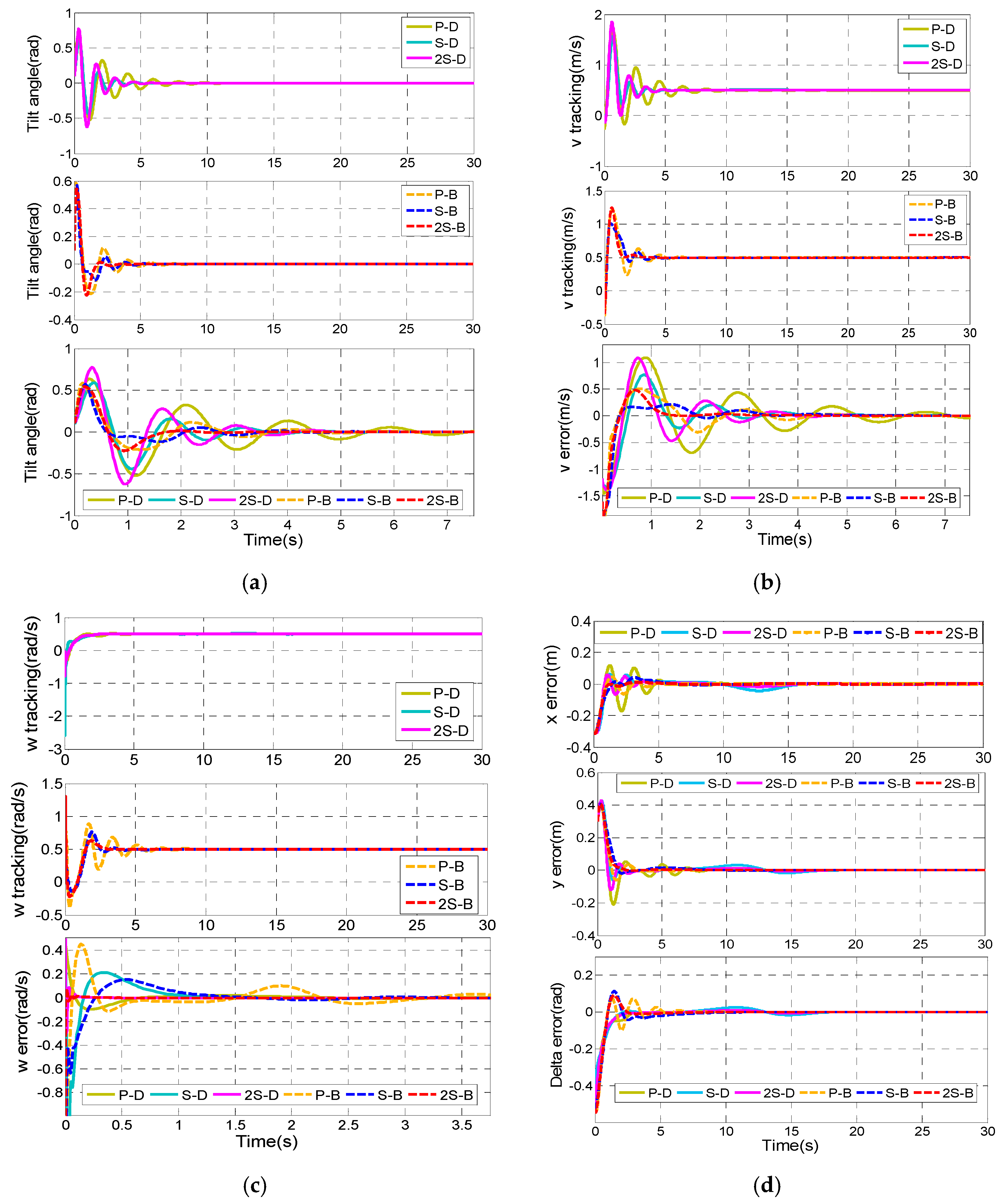
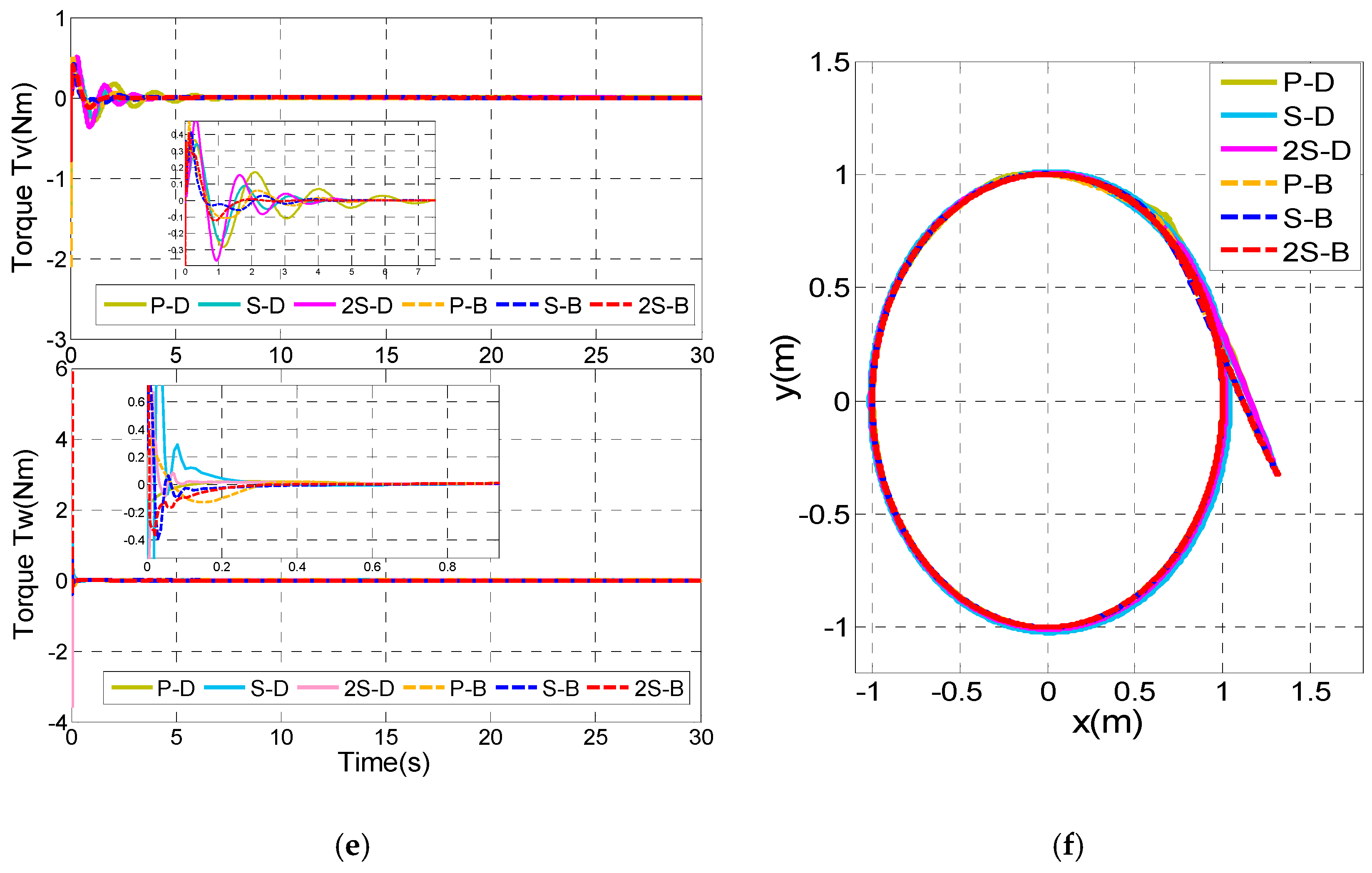
First, a reference circular trajectory with rad/s, m/s is given and the radius of the desired trajectory is 1 m. Furthermore, we assume that the vehicle start point is , and the initial state variables are supposed as . Figure 10 shows the practical tracking for the circle mentioned above with six different control combinations.
From Figure 10a, it is clearly shown that the 2S-B controller has the shortest settling time of the tilt angle (about 1.55 s), while the worst settling time of the tilt angle is about 7.06 s in the P-D controller. The tracking error of x decreases to zero after t = 0.95 s by the 2S-B controller. When it comes to the P-D controller, the tracking error of x has the longest settling time of 4.44 s (Figure 10d). Moreover, the overshoots of θ and in the 2S-B controller are smallest among them. Figure 10d indicates that the DMLF method has better response about the tracking error of δ, but worse performances of and than the backstepping method. Considering these simulation results, the 2S-B controller is the most effective control combination strategy.
To further verify the effectiveness of the proposed controllers, a more sophisticated trifolium trajectory is used as a reference trajectory.
A trifolium trajectory can be designed as , . Here, the desired length of each leaf ρ is chosen as ρ = 5, = 0.05. Then, the reference longitudinal velocity and the reference rotational velocity can be calculated in prior. Furthermore, we assume that the vehicle start point is , and the initial state variables are the same as that of tracking a circle.
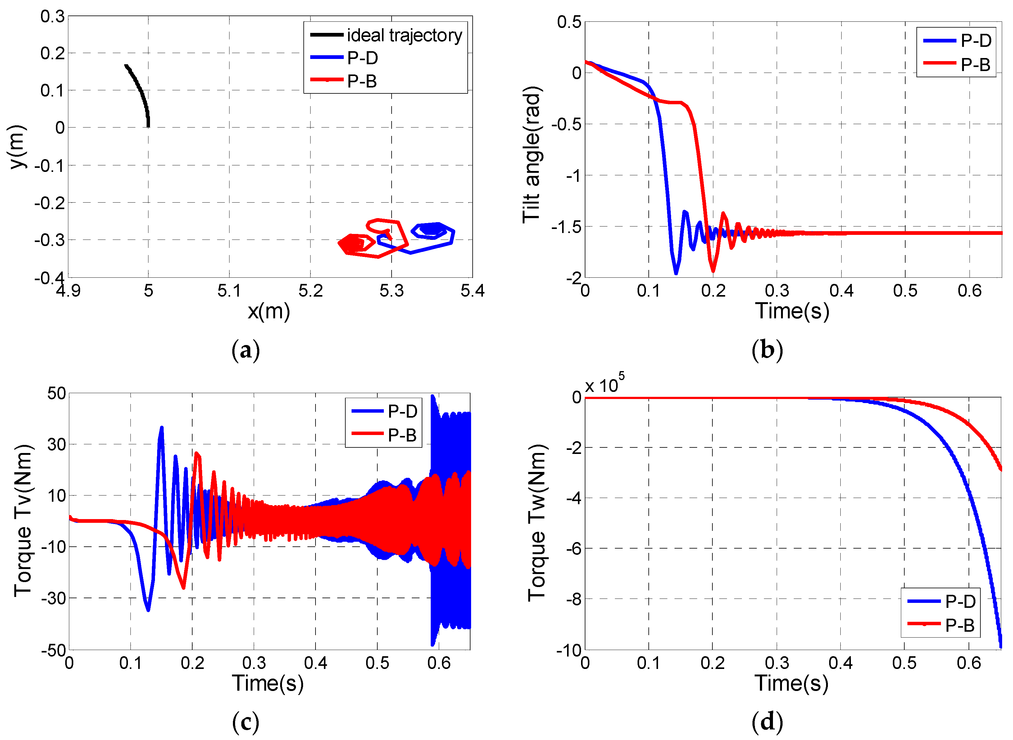
The system states are divergent for tracking a trifolium trajectory using the P-D controller and P-B controller. The reason why it diverges is the error of the longitudinal velocity converges more slowly than the acceleration of the reference longitudinal velocity . Moreover, the simulation results are shown in the Appendix A.
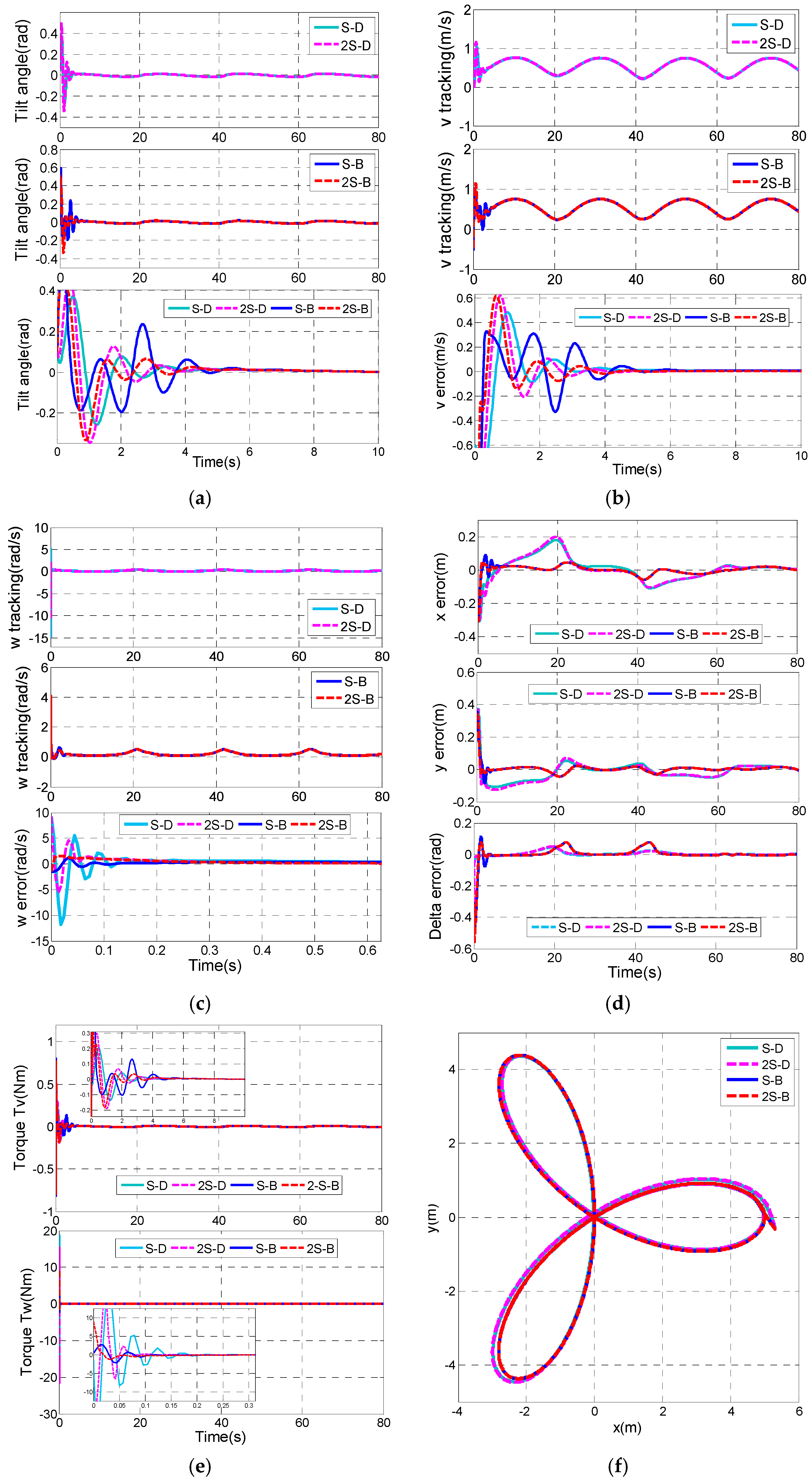
Figure 11 shows the comparison information of the four remaining control combinations, S-D controller, 2S-D controller, S-B controller and 2S-B controller.
It is clearly shown in Figure 11a that the S-D controller has the shortest settling time of the tilt angle (about 2.3 s), while the longest settling time of the tilt angle is about 4.37 s in the S-B controller. In Figure 11e, S-D and 2S-D have high rotational control torque up to around 20 Nm, while the rotational control torque in S-B controller is smaller than 2 Nm. The tracking errors of x and y are much smaller in the S-B controller and 2S-B controller than those of the S-D controller and 2S-D controller (Figure 11d). Moreover, the overshoots of and in the 2S-B controller are smallest among them.
Finally, a hexagon trajectory, which contains an abrupt variation of longitudinal velocity and rotational velocity, is more difficult to track than the trifolium one. The hexagon trajectory we adopt is described by piecewise linear functions. Furthermore, assume that the vehicle start point is , and the initial state variables are set as .
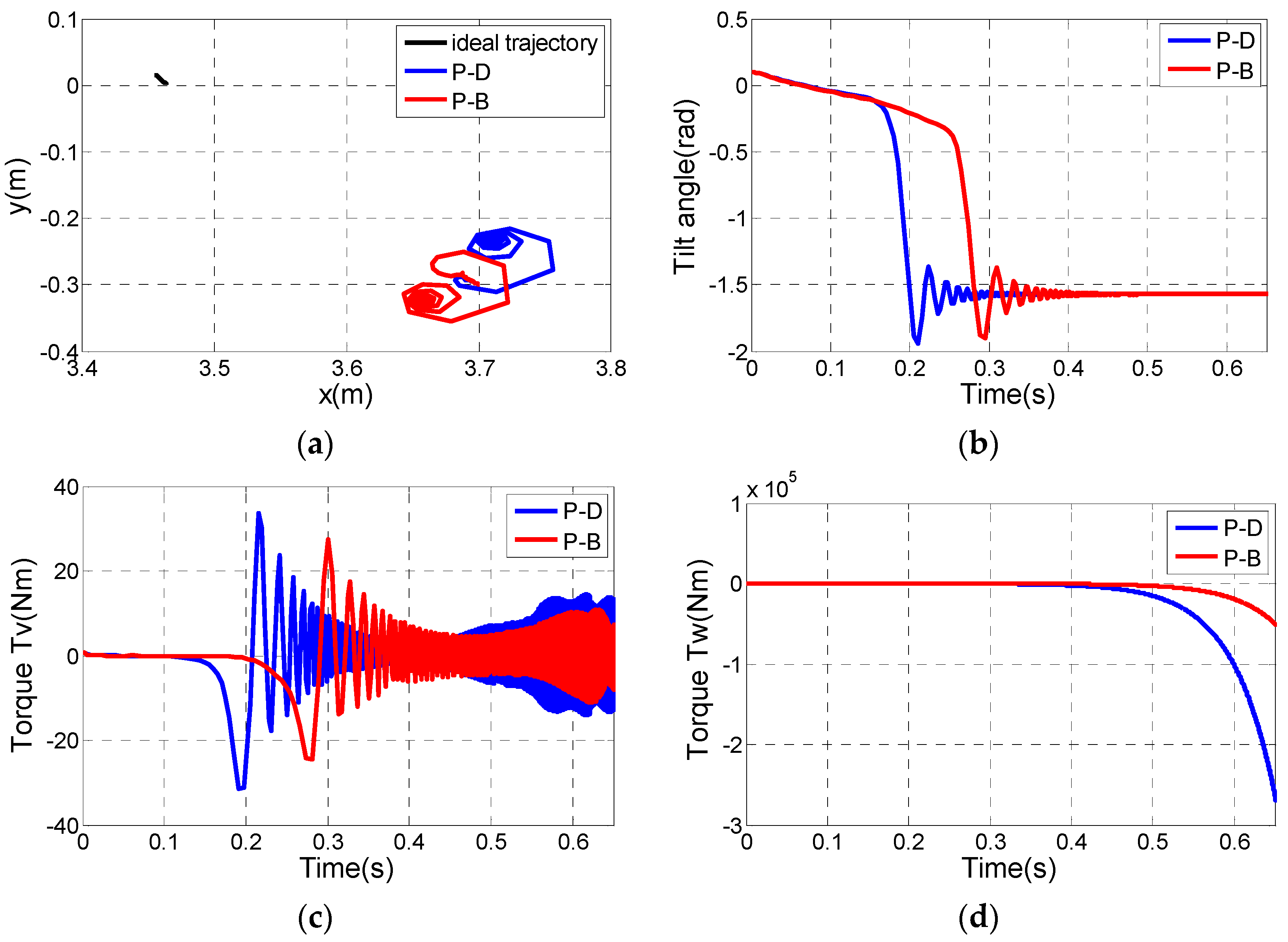
Similarly, the system states are divergent for tracking a hexagon using P-D controller and P-B controller. Moreover, the simulation results are shown in the Appendix A. Figure 12 shows the practical tracking performances for the hexagon mentioned above with four different control combinations.
Figure 12c shows that the 2S-B controller has the shortest settling time of the tilt angle (about 2.3 s), while the longest settling time of the tilt angle is about 3.3 s in the S-D controller. The tracking errors of x and y decrease most quickly to zero in the 2S-B controller. When it comes to the S-D controller and 2S-D controller, the settling time of and is up to about 7 s (Figure 12d). Moreover, the overshoots of , and in the 2S-B controller are the smallest.
Although the hexagon trajectory seems to be tracked effectively, the torque performance is actually terrible due to the abrupt variation of the trajectory of longitudinal velocity and rotational velocity, and this situation is undesirable in practice.
Table 7 shows the different control effects of the six control combinations, such as the overshoot and the settling time of θ, , , , and a coincidence factor indicator (CFI) which illustrates the trajectory tracking performance.
We define a coincidence factor indicator (CFI) to describe the tracking performance. The CFI is obtained as follows:
where, ()* means the normalization of expressions in brackets, min is the minimum of from i = 1 to i = N, max is the maximum of from i = 1 to i = N, is the number of samples, and T is the total time of simulation.
Different control effects of the six control combinations are clearly shown in Table 7, where we can see that the P-D and the P-B controller have poor adaptability to different trajectories. The convergence rates of , and are much faster by using the backstepping method than using the DMLF method. It can be clearly seen that 2S-B method has the best CFI as well as shortest settling time of the tilt angle for all three trajectories, so it can be concluded that among the six control combinations, 2S-B controller has the best control performance for its fast convergence speed, small overshoot and best trajectory coincidence.
6. Experimental Results
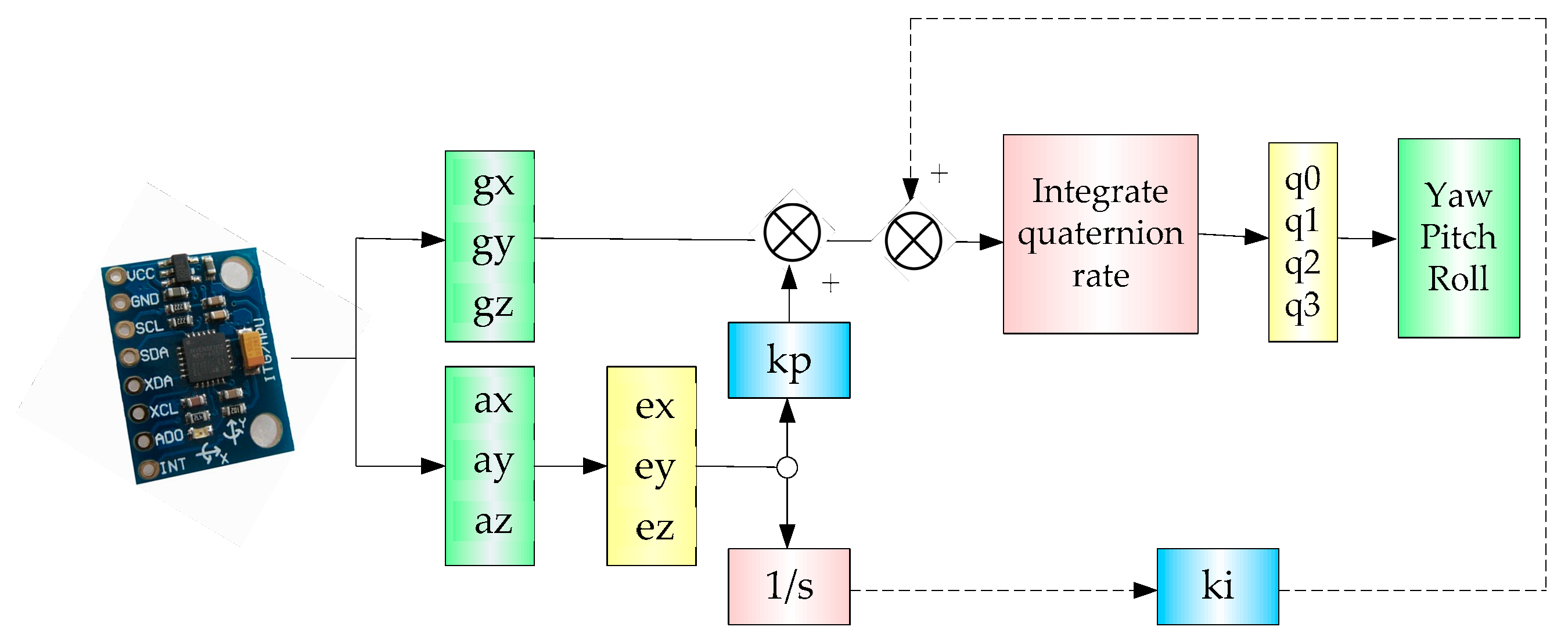
Since the sensor (MPU-6050) has an embedded 3-axis MEMS gyroscope and a 3-axis MEMS accelerometer, we need to utilize an information fusion algorithm to obtain relatively accurate information. Figure 13 shows the frame of the complementary filter for information fusion.
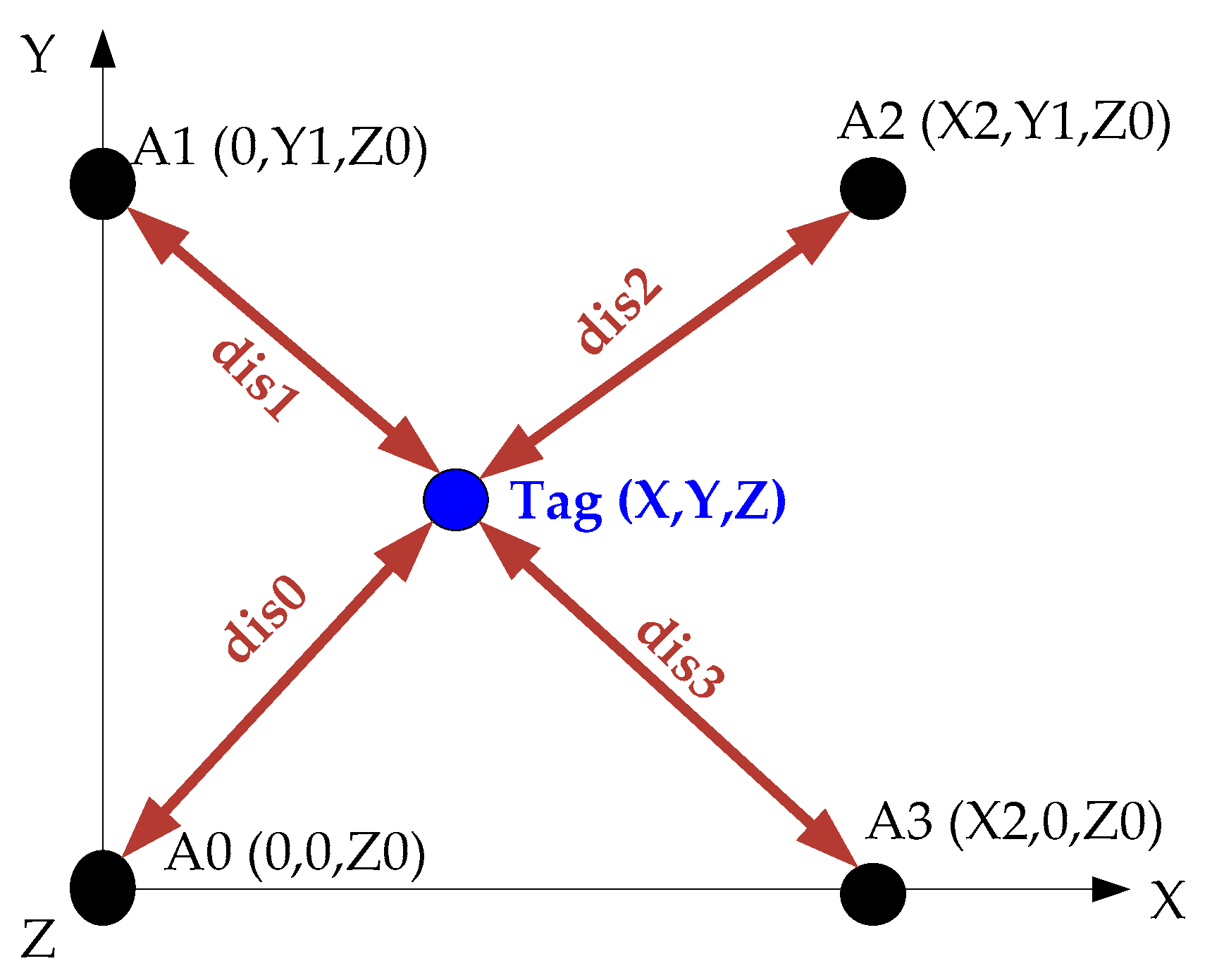
The attitude data of the TWIP vehicle is measured via the onboard IMU, the velocity data is measured by two rotary encoders, and the location information of the TWIP vehicle is measured by the UWB positioning technology just as shown in Figure 2. The placement of anchors in space is shown in Figure 14.
The position of the Tag can be expressed as follows:
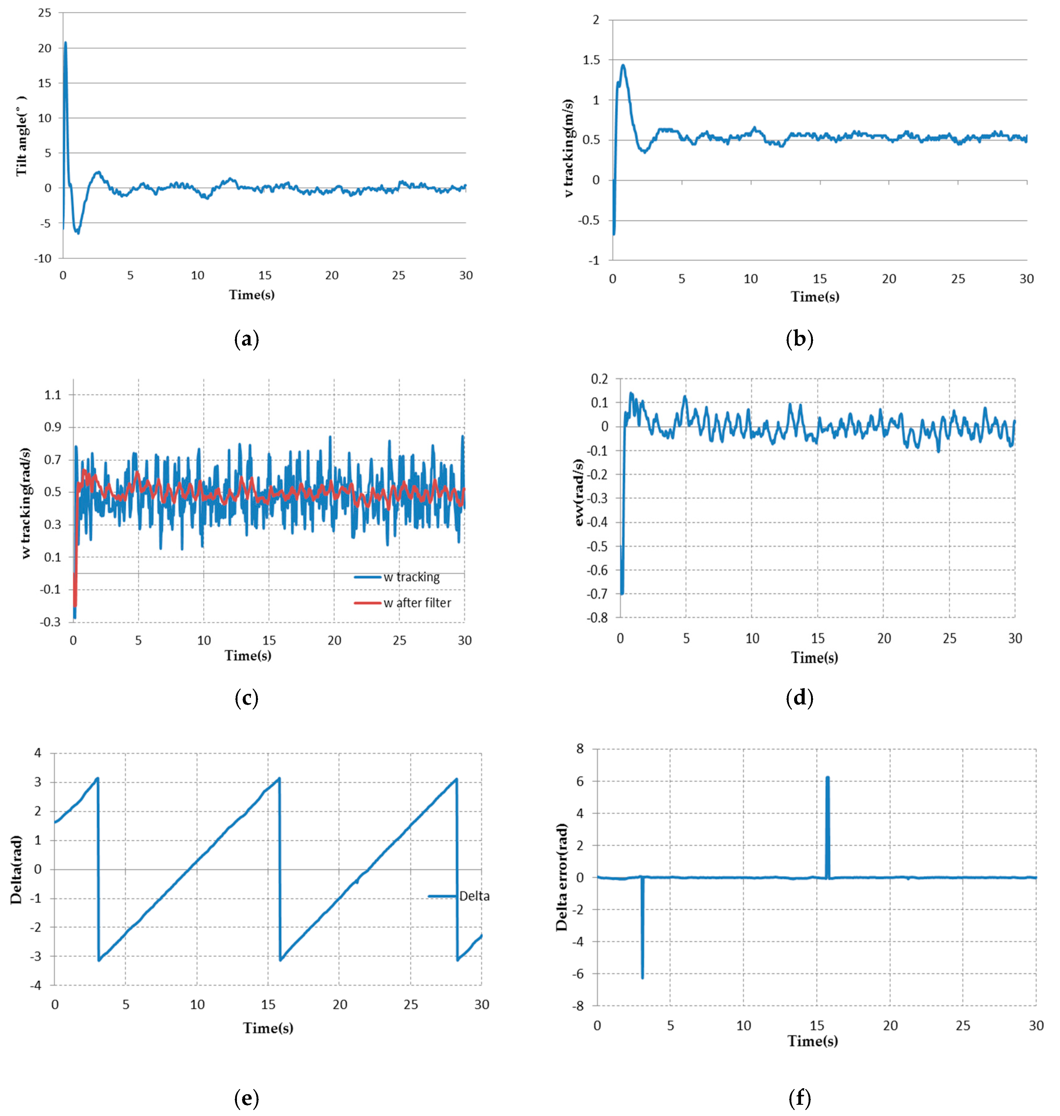
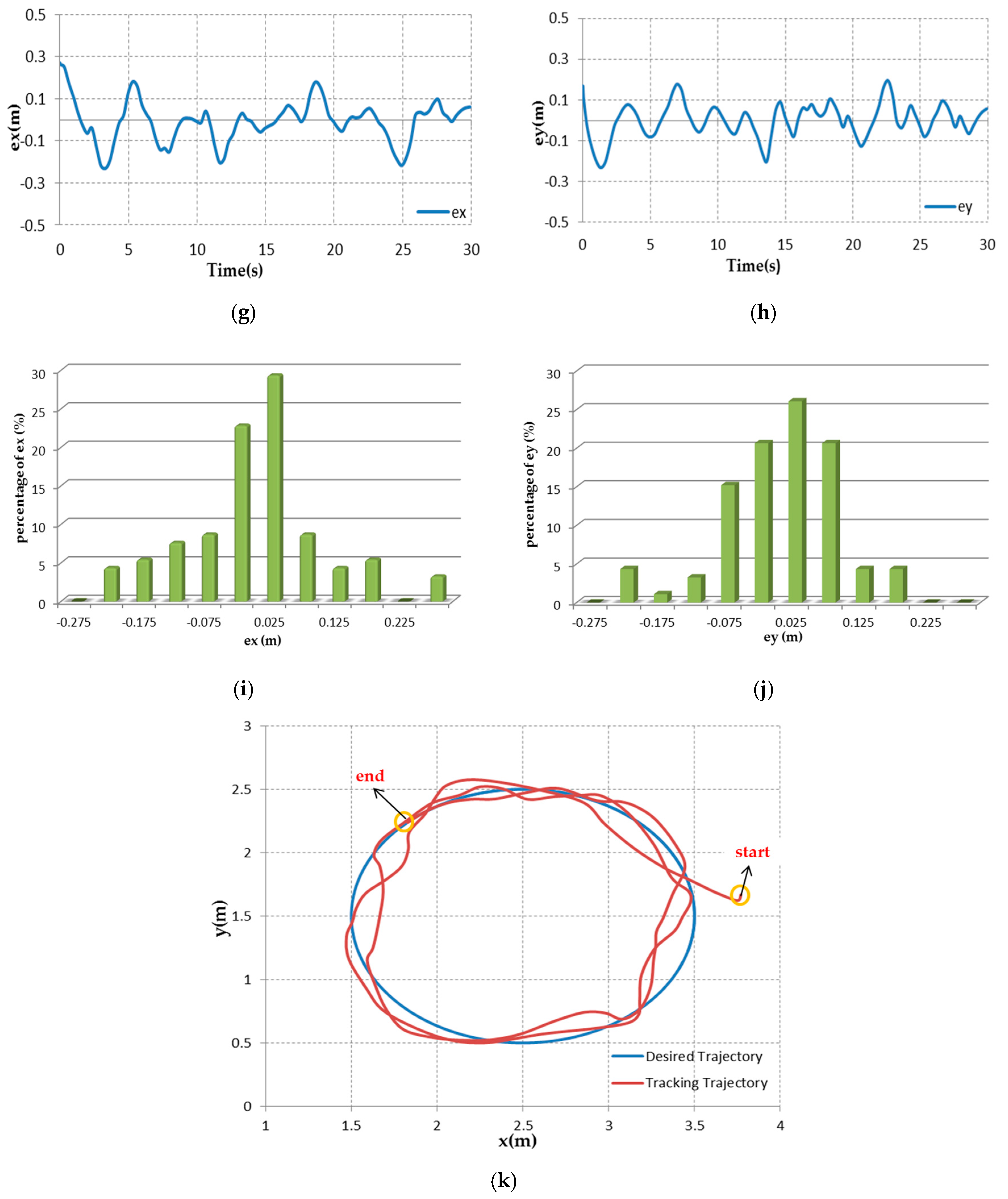
To verify the tracking performance of the proposed design, an indoor tracking test was implemented. The desired trajectory was set to be a circle with rad/s, m/s. The radius of the desired trajectory was 1 m. Considering the existence of mismatch between the real-time system model and the mathematical model, the feedback gains obtained from simulations may not function well on the real-time platform, thus the control design parameters need to be adjusted through experiments on the prototype. In practice, we use the control design parameters as Figure 15 shows the indoor experimental results using the 2S-B controller for tracking the circle.
After the battery is fully charged, the TWIP vehicle can run continuously for about 30 min. The test of tracking a circle lasts about 30 s, and the TWIP vehicle finished the trajectory tracking for more than two rounds. Figure 15a shows the tilt angle of the TWIP vehicle. Figure 15g,h shows the position tracking errors. Because there is a cm-level measure error in the position measurement by UWB technology, the position tracking errors cannot converge to zero. The maximum position tracking error is about ±0.27 m for x-direction and about ±0.23 m for y-direction, but more than 80% of the all recorded horizontal points remain in a circle with a radius of 0.1 m. The RMS value of the position error is 0.1036 m in x-direction, and 0.0841 m in y-direction. The settling time of the tilt angle is about 3.5 s. Td the tilt angle is controlled within ±1.5°. This demonstrates the good tracking performance achieved in the indoor environment.
7. Conclusions
In this paper, an inner/outer loop control is proposed for the trajectory control of a TWIP vehicle. Several control methods have been utilized in the inner or outer loop controller and then different control combinations of inner and outer loop control methods have been proposed. A lot of simulations have been conducted to compare the control performance of different control combinations. Then, the simulation results illustrate that the 2S-B combination has the most effective control performance and highly adaptability to different trajectories. Finally experiments have been carried out to verify the effectivity of the 2S-B combination. In our future work, the Kalman filter and its variants will be considered to obtain the state estimation such that the effects of sensor noises can be attenuated. Further investigation will be conducted on path-planning arithmetic for environment exploration.
Acknowledgments
This work was supported in part by National Natural Science Foundation (Nos. 61571127, 61001048), Key Laboratory of Micro-Inertial Instrument and Advanced Navigation Technology, Ministry of Education, China (Project No. KL201102), Major Project Guidance Foundation of Basic Scientific Research Operation Expenses, Southeast University (No. 3222003104), Natural Science Fund of Jiangsu Province (BK20131295, BK20130636), Aeronautical Science Foundation of China (No. 20160869004).
Author Contributions
Dun-Zhu Xia conceived the topic and developed the model; Yan-Hong Yao and Li-Mei Cheng finalized the simulation; Yan-Hong Yao analyzed the results; all authors wrote the paper.
Conflicts of Interest
The authors declare no conflict of interest.
Appendix A
Figure A2a–d illustrate that the system states are divergent for tracking a trifolium trajectory using the P-D controller and P-B controller. Compared with the circle trajectory, the trifolium trajectory is more sophisticated and the tracking velocity changes rapidly at the beginning.
Figure A3a–d illustrate that the system states are divergent for tracking a hexagon using the P-D controller and P-B controller. Comparing with the circle trajectory, the hexagon trajectory is more sophisticated and the tracking velocity and changes rapidly at the beginning.
Figure A1.
Simulation framework for 2S-B controller.
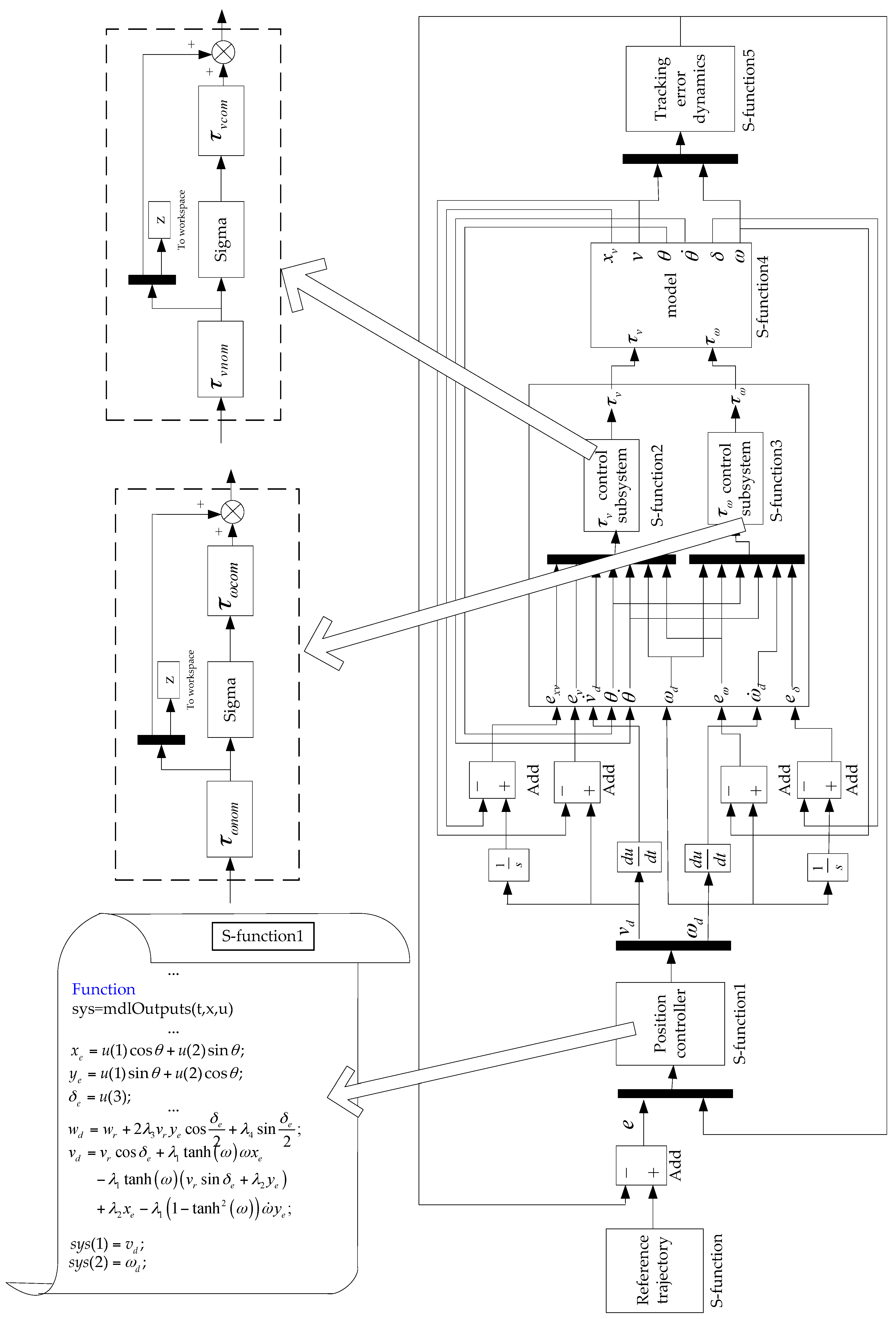
Figure A2.
Control peformance of PID&Backstepping controller and PID&DMLF controller for tracking a trifolium, (a) Tracking trajectories; (b) Tilt angle of the TWIP vehicle; (c,d) Control torques and .
Figure A2.
Control peformance of PID&Backstepping controller and PID&DMLF controller for tracking a trifolium, (a) Tracking trajectories; (b) Tilt angle of the TWIP vehicle; (c,d) Control torques and .

Figure A3.
Control peformance of PID&Backstepping controller for tracking a hexagon, (a) Tracking trajectories; (b) Tilt angle of the TWIP vehicle; (c,d) Control torques and .
Figure A3.
Control peformance of PID&Backstepping controller for tracking a hexagon, (a) Tracking trajectories; (b) Tilt angle of the TWIP vehicle; (c,d) Control torques and .

References
- Isidori, A.; Marconi, L.; Serrani, A. Robust Autonomous Guidance: An Internal Model Approach; Springer: London, UK, 2003; ISBN 978-1-4471-1124-5. [Google Scholar]
- Yang, C.; Li, Z.; Cui, R.; Xu, B. Neural network-based motion control of an underactuated wheeled inverted pendulum model. IEEE Trans. Neural Netw. Learn. Syst. 2014, 25, 2004–2016. [Google Scholar] [CrossRef] [PubMed]
- Nomura, T.; Kitsuka, Y.; Suemitsu, H.; Matsuo, T. Adaptive Backstepping Control for a Two-Wheeled Autonomous Robot. In Proceedings of the ICCAS-SICE, Fukuoka, Japan, 18–21 August 2009; pp. 4687–4692. [Google Scholar]
- Tsai, C.C.; Huang, H.C.; Lin, S.C. Adaptive neural network control of a self-balancing two-wheeled scooter. IEEE Ind. Electron. Trans. 2010, 57, 868–873. [Google Scholar] [CrossRef]
- Capisani, L.M.; Ferrara, A.; Magnani, L. Design and experimental validation of a second-order sliding-mode motion controller for robot manipulators. Int. J. Control 2009, 82, 365–377. [Google Scholar] [CrossRef]
- Chen, H.Y.; Liang, J.W.; Wu, J.W. Active pneumatic vibration control by using pressure and velocity measurements and adaptive fuzzy sliding-mode controller. Sensors 2012, 13, 8431–8444. [Google Scholar] [CrossRef] [PubMed]
- Utkin, V.I.; Lee, H. The chattering analysis. Lect. Notes Control Inf. Sci. 2006, 334, 2014–2019. [Google Scholar] [CrossRef]
- Khan, M.K.; Spurgeon, S.K. Robust mimo water level control in interconnected twin-tanks using second order sliding mode control. Control Eng. Pract. 2006, 14, 375–386. [Google Scholar] [CrossRef]
- Nollet, F.; Floquet, T.; Perruquetti, W. Observer-based second order sliding mode control laws for stepper motors. Control Eng. Pract. 2008, 16, 429–443. [Google Scholar] [CrossRef]
- Levant, A. Sliding order and sliding accuracy in sliding mode control. Int. J. Control 1993, 58, 1247–1263. [Google Scholar] [CrossRef]
- Nakano, S.; Ibuki, T.; Sampei, M. Visual feedback pose tracking control of two-wheeled vehicles with target vehicle motion models. In Proceedings of the 55th Annual Conference of the Society of Instrument and Control Engineers of Japan (SICE), Tsukuba, Japan, 20–23 September 2016; pp. 1070–1075. [Google Scholar]
- Fontana, R.J. Recent system applications of short-pulse ultra-wideband (UWB) technology. IEEE Trans. Microw. Theory Tech. 2004, 52, 2087–2104. [Google Scholar] [CrossRef]
- Fontana, R.J.; Richley, E.; Barney, J. Commercialization of an ultra wideband precision asset location system, Ultra Wideband Systems and Technologies. In Proceedings of the IEEE Conference, Reston, VA, USA, 16–19 November 2003; pp. 369–373. [Google Scholar] [CrossRef]
- Xia, D.; Kong, L.; Hu, Y.; Ni, P. Silicon microgyroscope temperature prediction and control system based on BP neural network and fuzzy-PID control method. Meas. Sci. Technol. 2015, 26, 025101. [Google Scholar] [CrossRef]
- Yang, X.M.; Gao, Y.P. High-order adaptive super-twisting sliding mode control for uncertain underactuated systems. Pattern Recognit. Artif. Intell. 2014, 27, 808–814. [Google Scholar] [CrossRef]
- Yue, M.; Wang, S.; Sun, J.Z. Simultaneous balancing and trajectory tracking control for two-wheeled inverted pendulum vehicles: A composite control approach. Neurocomputing 2016, 191, 44–54. [Google Scholar] [CrossRef]
- Li, P.; Zheng, Z.Q. Convergence of super-twisting algorithm based on quadratic-like Lyapunov function. Control Decis. 2011, 26, 949–952. [Google Scholar]
- Kamal, S.; Chalanga, A.; Moreno, J.A.; Fridman, L. Higher order super-twisting algorithm. In Proceedings of the 13th International Workshop on Variable Structure Systems, Nantes, France, 29 June–2 July 2014; pp. 1–5. [Google Scholar] [CrossRef]
- Liu, J.; Wang, X. Advanced Sliding Mode Control for Mechanical Systems: Design, Analysis and Matlab Simulation; Springer-Verlag: Berlin/Heidelberg, Germany, 2011; ISBN 978-3-642-20906-2. [Google Scholar]
- Hwang, C.L.; Chiang, C.C.; Yeh, Y.W. Adaptive fuzzy hierarchical sliding-mode control for the trajectory tracking of uncertain underactuated nonlinear dynamic systems. IEEE Trans. Fuzzy Syst. 2014, 22, 286–299. [Google Scholar] [CrossRef]
- Yu, X.; Lu, Z. Hierarchical sliding-mode control of bicycle robot system. In Proceedings of the International Conference on Computer Science and Service System (CSSS), Nanjing, China, 27–29 June 2011; pp. 3260–3263. [Google Scholar]
- Hespanha, J.P. Uniform stability of switched linear systems: Extensions of lasalle's invariance principle. IEEE Trans. Autom. Control 2004, 49, 470–482. [Google Scholar] [CrossRef]
- Lo, J.C.; Kuo, Y.H. Decoupled fuzzy sliding-mode control. IEEE Trans. Fuzzy Syst. 1998, 6, 426–435. [Google Scholar] [CrossRef]
- Zhang, L.; Shi, P. Model reduction for switched lpv systems with average dwell time. IEEE Trans. Autom. Control 2008, 53, 2443–2448. [Google Scholar] [CrossRef]
Figure 1.
The experimental two-wheeled inverted pendulum vehicle.
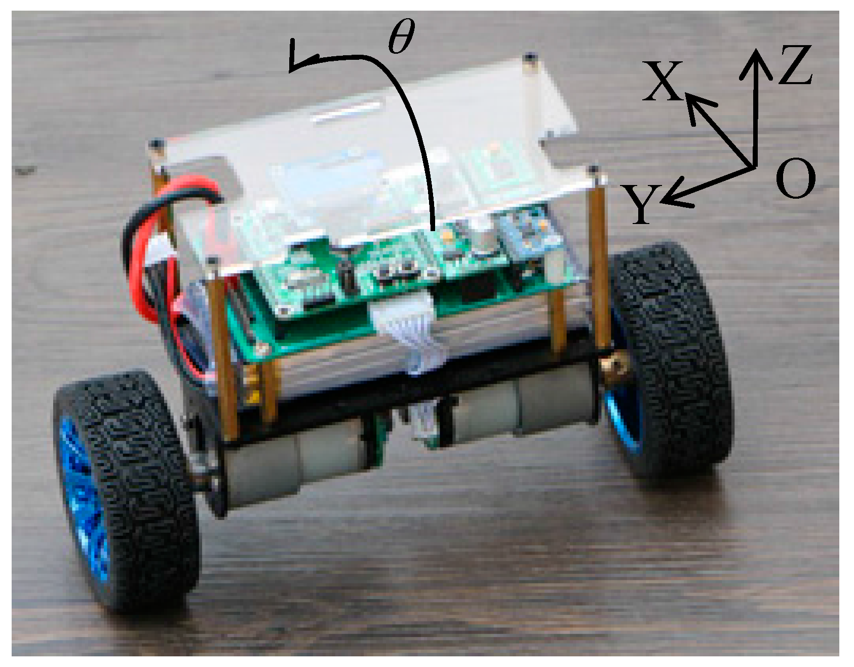
Figure 2.
System architecture.
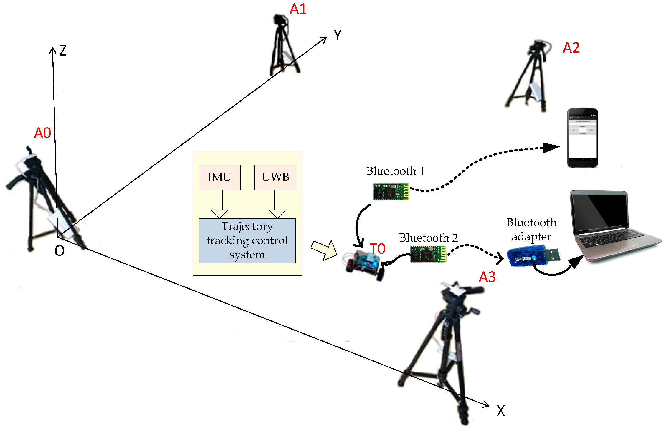
Figure 3.
The fixed coordinate system of the vehicle: (a) A simplified schematic diagram; (b) Motion of the vehicle on the x-y plane.
Figure 3.
The fixed coordinate system of the vehicle: (a) A simplified schematic diagram; (b) Motion of the vehicle on the x-y plane.
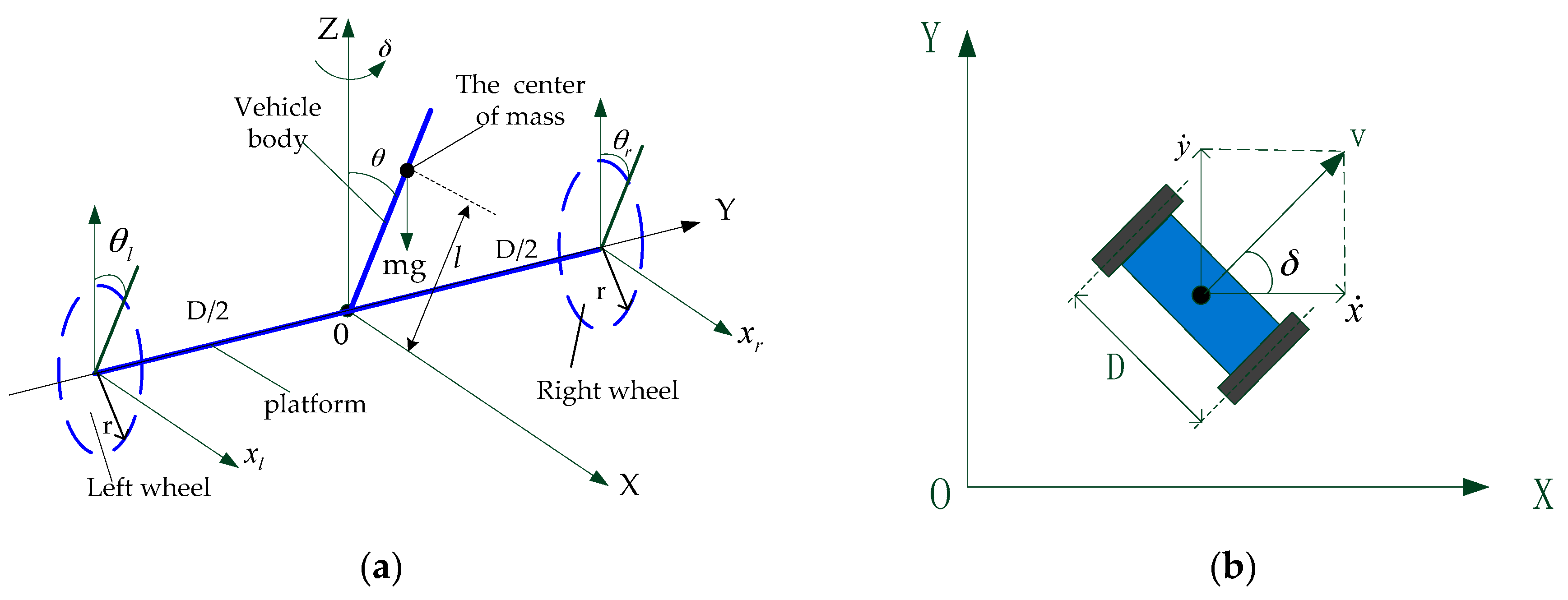
Figure 4.
The structure of the inner/outer loop control system.
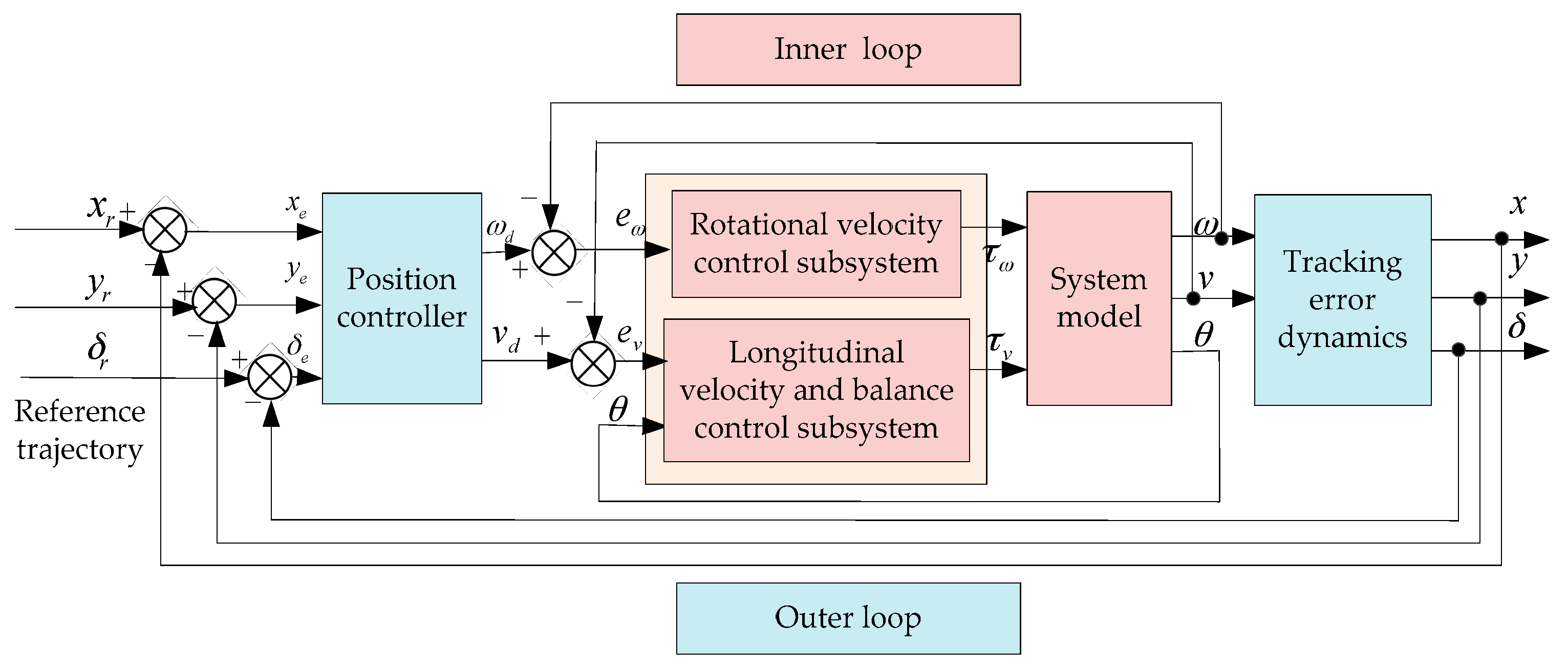
Figure 5.
Comparison results of the controller with different control parameters. (a) v tracking error; (b) ω tracking error; (c) Tilt angle of the TWIP vehicle; (d) The longitudinal control input and the rotational control input .
Figure 5.
Comparison results of the controller with different control parameters. (a) v tracking error; (b) ω tracking error; (c) Tilt angle of the TWIP vehicle; (d) The longitudinal control input and the rotational control input .
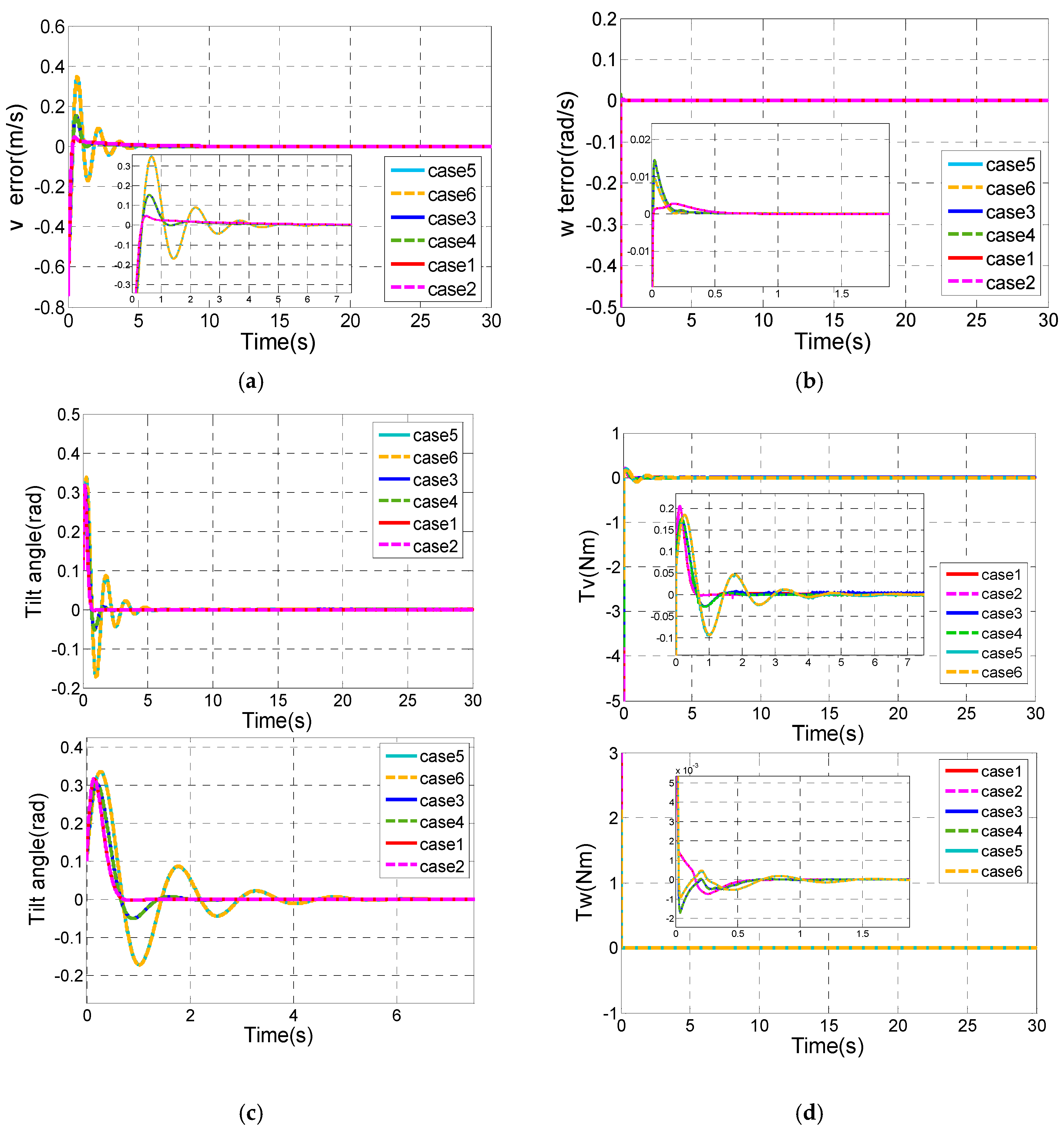
Figure 6.
The control performances of case1 and case2 with system uncertainty. (a) v tracking error; (b) ω tracking error; (c) Tilt angle of the TWIP vehicle; (d) The longitudinal control input ; (e) The rotational control input ; (f) r1 of case1; (g) r1 of case2; (h) r2 of case1 and case2.
Figure 6.
The control performances of case1 and case2 with system uncertainty. (a) v tracking error; (b) ω tracking error; (c) Tilt angle of the TWIP vehicle; (d) The longitudinal control input ; (e) The rotational control input ; (f) r1 of case1; (g) r1 of case2; (h) r2 of case1 and case2.


Figure 7.
Comparison results of the two controllers with system uncertainty. (a) Tilt angle of the TWIP vehicle; (b) v tracking; (c) ω tracking ; (d) The adaptive value of 2-RASMC; (e) The longitudinal control input ; (f) The rotational control input .
Figure 7.
Comparison results of the two controllers with system uncertainty. (a) Tilt angle of the TWIP vehicle; (b) v tracking; (c) ω tracking ; (d) The adaptive value of 2-RASMC; (e) The longitudinal control input ; (f) The rotational control input .


Figure 8.
Comparison results of the two controllers with system uncertainty. (a) Tilt angle of the TWIP vehicle; (b) v tracking; (c) ω tracking ; (d) The adaptive value of 2-RASMC; (e) The longitudinal control input ; (f) The rotational control input .
Figure 8.
Comparison results of the two controllers with system uncertainty. (a) Tilt angle of the TWIP vehicle; (b) v tracking; (c) ω tracking ; (d) The adaptive value of 2-RASMC; (e) The longitudinal control input ; (f) The rotational control input .


Figure 9.
The posture errors of the two-wheeled vehicle.
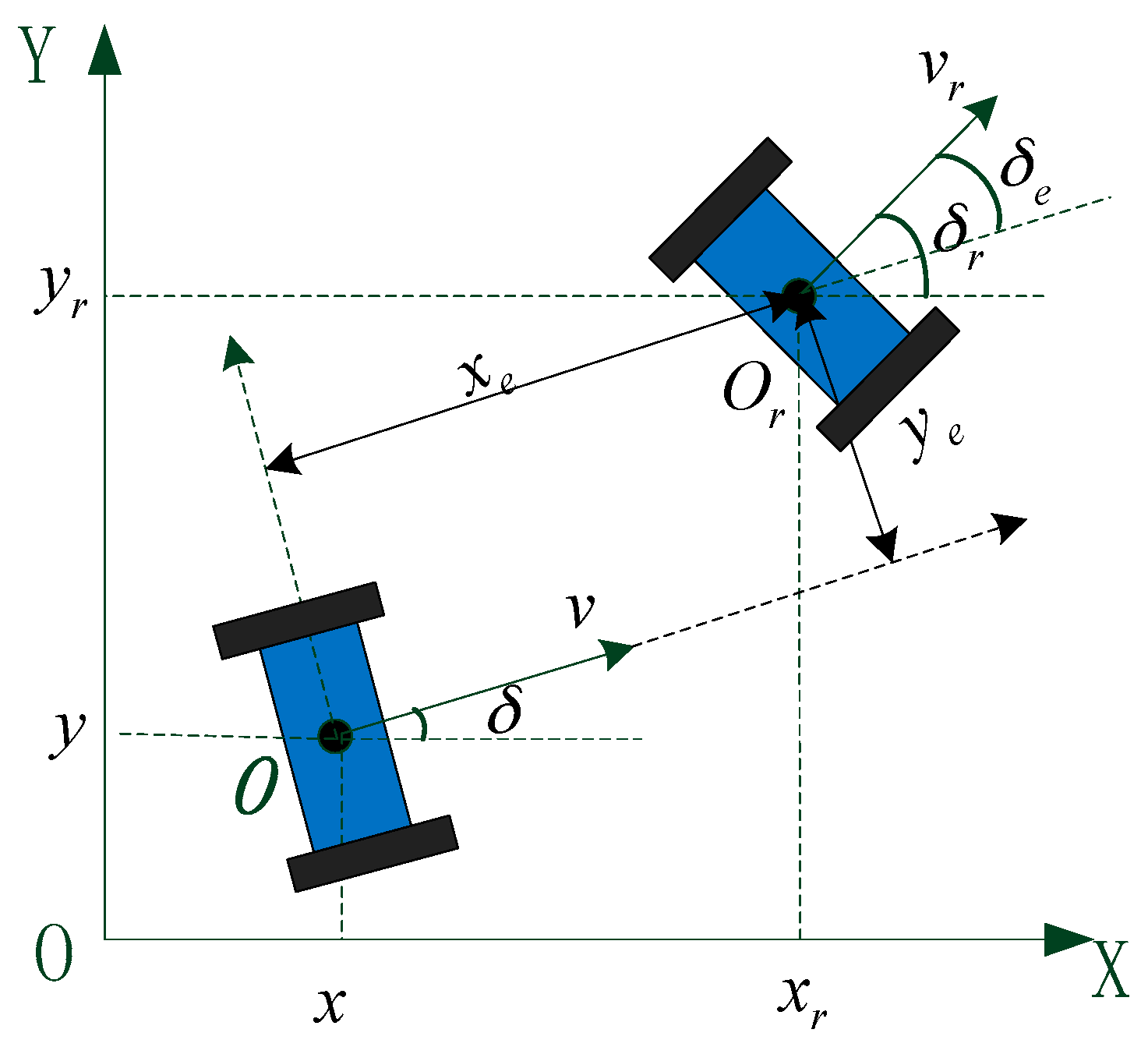
Figure 10.
Comparison results of control combinations. (a) Tilt angle of the TWIP vehicle; (b) v tracking; (c) ω tracking ; (d) Tracking errors of x, y and δ; (e) Longitudinal control input and rotational control input ; (f) Tracking of the circle trajectory.
Figure 10.
Comparison results of control combinations. (a) Tilt angle of the TWIP vehicle; (b) v tracking; (c) ω tracking ; (d) Tracking errors of x, y and δ; (e) Longitudinal control input and rotational control input ; (f) Tracking of the circle trajectory.


Figure 11.
Comparison results of control combinations. (a) Tilt angle of the TWIP vehicle; (b) v tracking; (c) ω tracking ; (d) Tracking errors of x, y and δ; (e) Longitudinal control input and rotational control input ; (f) Tracking of the trifolium trajectory.
Figure 11.
Comparison results of control combinations. (a) Tilt angle of the TWIP vehicle; (b) v tracking; (c) ω tracking ; (d) Tracking errors of x, y and δ; (e) Longitudinal control input and rotational control input ; (f) Tracking of the trifolium trajectory.

Figure 12.
Comparison results of control combinations. (a) v tracking; (b) ω tracking ; (c) Tilt angle of the TWIP vehicle; (d) Tracking errors of x, y and δ; (e) Longitudinal control input and rotational control input ; (f) Tracking of the hexagon trajectory.
Figure 12.
Comparison results of control combinations. (a) v tracking; (b) ω tracking ; (c) Tilt angle of the TWIP vehicle; (d) Tracking errors of x, y and δ; (e) Longitudinal control input and rotational control input ; (f) Tracking of the hexagon trajectory.
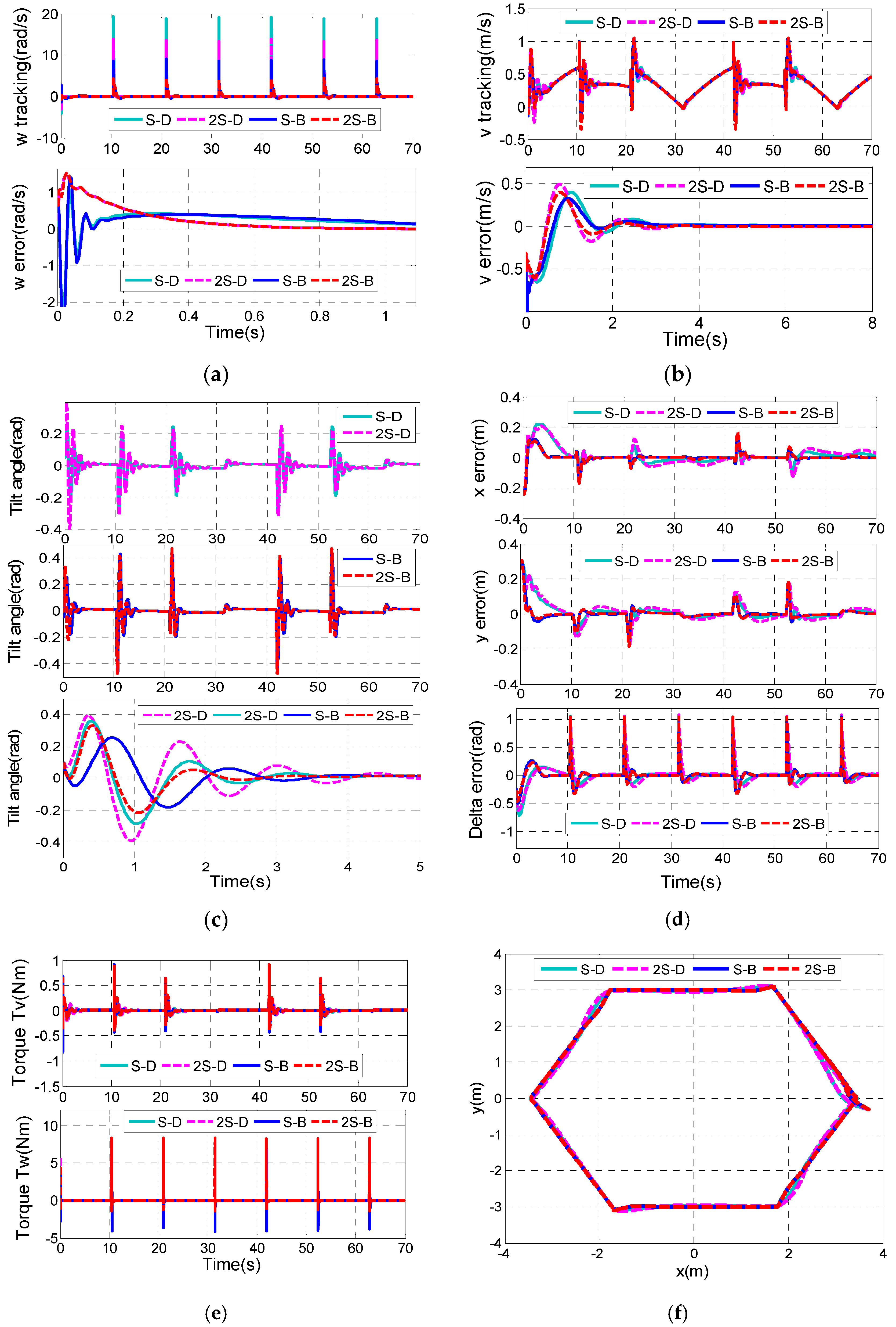
Figure 13.
The frame of multi-sensor information fusion algorithm.

Figure 14.
The placement of anchors in space.

Figure 15.
Experimental results of tracking for a circle. (a) Tilt angle of the TWIP vehicle; (b,c) v and ω tracking; (d) ω tracking error; (e) δ tracking; (f–h) Tracking errors of δ, x, y respectively; (i,j) Histograms of tracking errors of x, y respectively; (k) Practical tracking trajectory.
Figure 15.
Experimental results of tracking for a circle. (a) Tilt angle of the TWIP vehicle; (b,c) v and ω tracking; (d) ω tracking error; (e) δ tracking; (f–h) Tracking errors of δ, x, y respectively; (i,j) Histograms of tracking errors of x, y respectively; (k) Practical tracking trajectory.


Table 1.
The parameters and variables of two-wheeled inverted pendulum vehicle system.
| Parameter and Variable Name | Symbol | Value (Unit) |
|---|---|---|
| Acceleration due to gravity | g | 9.8 (m/s2) |
| Mass of the wheel | MW | 0.03 (kg) |
| Mass of the body | m | 2 (kg) |
| Radius of the wheel | r | 0.04 (m) |
| Length between the wheel axle and the center of gravity of the body | 0.1 (m) | |
| Rotational inertia of the wheel | JW | 3.17 × 10⁻⁵ (kg·m2) |
| Rotational inertia of the body about the Y-axis | Jθ | 0.003 (kg·m2) |
| Rotational inertia of the body about the Z-axis | Jδ | 0.002 (kg·m2) |
| Distance between the two wheels along the axle center | D | 0.17 (m) |
| Tilt angle of the vehicle body | θ | (rad) |
| The angle wheels turned | θr, θl | (rad) |
| Heading angle of the vehicle | δ | (rad) |
| Output torques of left and right wheel DC motors | τr, τl | (Nm) |
| Longitudinal displacement along the movement direction | XV | (m) |
| Longitudinal velocity of the vehicle | v | (m/s) |
| Rotational velocity of the vehicle | ω | (rad/s) |
Table 2.
The designed parameters of the 2-RASMC controller.
| Control Parameter | ||||||||||
|---|---|---|---|---|---|---|---|---|---|---|
| Case1 | 5 | 0.4 | 4 | 4 | 5 | 12 | 10 | 15 | 3 | 3 |
| Case2 | 5 | 0.4 | 4 | 4 | 5 | 12 | 10 | 15 | 1/8 | 1/3 |
| Case3 | 5 | 0.5 | 3 | 3 | 3 | 5 | 10 | 15 | 3 | 3 |
| Case4 | 5 | 0.5 | 3 | 3 | 3 | 5 | 10 | 15 | 1/8 | 1/3 |
| Case5 | 0.5 | 0.5 | 3 | 3 | 3 | 5 | 3 | 5 | 3 | 3 |
| Case6 | 0.5 | 0.5 | 3 | 3 | 3 | 5 | 3 | 5 | 1/8 | 1/3 |
Table 3.
The designed parameters of the inner loop controller.
| Control Parameter | ||||||||||
|---|---|---|---|---|---|---|---|---|---|---|
| 2-SMC | 5 | 0.4 | 4 | 4 | 5 | 12 | 10 | 15 | -- | -- |
| 2-RASMC | 5 | 0.4 | 4 | 4 | 5 | 12 | 10 | 15 | 1/8 | 1/3 |
Table 4.
The design parameters of the outer loop controller.
| Design Parameters | ||||
|---|---|---|---|---|
| Value | 1 | 1 | 20 | 5 |
Table 5.
Several algorithmic approaches of the inner/outer loop control system.
| Outer Loop Controller | Direct Method of Lyapunov Function (DMLF) [16] | Backstepping | |
|---|---|---|---|
| Inner Loop Controller | |||
| PID | P-D controller | P-B controller | |
| SMC [19] | S-D controller | S-B controller | |
| 2-RASMC | 2S-D controller | 2S-B controller | |
Table 6.
Control parameters of the PID controller.
| Control Parameter | |||||||||
|---|---|---|---|---|---|---|---|---|---|
| Value | 0.6 | 0.6 | 0.3 | 1.5 | 0 | 1.5 | 3 | 0 | 0.5 |
Table 7.
The key performance indicators of three different control combinations.
| Trajectory | Key Performance Indicators | DMLF | Backstepping | |||||
|---|---|---|---|---|---|---|---|---|
| PID | SMC | 2-SMC | PID | SMC | 2-SMC | |||
| Circle | θ | Overshoot σ (%) | 63.67 | 58.95 | 77.08 | 58.70 | 57.02 | 54.44 |
| Settling time (s) | 7.06 | 3.40 | 3.81 | 4.01 | 3.22 | 1.55 | ||
| Overshoot σ (%) | 11.75 | 6.03 | 5.75 | 4.52 | 4.08 | 0.96 | ||
| Settling time (s) | 4.44 | 2.90 | 2.64 | 2.77 | 3.58 | 0.95 | ||
| Overshoot σ (%) | 41.10 | 42.84 | 42.92 | 39.77 | 40.70 | 40.53 | ||
| Settling time (s) | 5.23 | 1.45 | 1.87 | 2.57 | 1.44 | 1.34 | ||
| Overshoot σ (%) | 0.19 | 2.38 | 0.95 | 7.23 | 11.21 | 8.96 | ||
| Settling time (s) | 2.43 | 1.58 | 1.72 | 3.96 | 4.09 | 2.05 | ||
| CFI (%) | 97.22 | 95.80 | 97.54 | 97.83 | 96.64 | 98.39 | ||
| Trifolium | θ | Overshoot σ (%) | -- | 37.52 | 49.43 | -- | 59.45 | 54.20 |
| Settling time (s) | -- | 2.30 | 2.63 | -- | 4.37 | 3.02 | ||
| Overshoot σ (%) | -- | 17.96 | 19.90 | -- | 9.01 | 4.80 | ||
| Settling time (s) | -- | -- | -- | -- | 3.79 | 2.13 | ||
| Overshoot σ (%) | -- | 12.35 | 10.80 | -- | 8.50 | 2.22 | ||
| Settling time (s) | -- | 24.59 | 25.87 | -- | 2.38 | 0.82 | ||
| Overshoot σ (%) | -- | 0.00 | 0.00 | -- | 11.32 | 7.65 | ||
| Settling time (s) | -- | 0.43 | 0.30 | -- | 3.25 | 2.30 | ||
| CFI (%) | -- | 88.51 | 86.13 | -- | 94.88 | 95.65 | ||
| Hexagon | θ | Overshoot σ (%) | -- | 23.19 | 39.63 | -- | 25.24 | 29.19 |
| Settling time (s) | -- | 3.27 | 3.30 | -- | 2.63 | 2.33 | ||
| Overshoot σ (%) | -- | 21.93 | 20.90 | -- | 11.97 | 11.48 | ||
| Settling time (s) | -- | 8.34 | 8.63 | -- | 4.18 | 4.15 | ||
| Overshoot σ (%) | -- | 0.00 | 0.00 | -- | 4.15 | 2.41 | ||
| Settling time (s) | -- | 6.98 | 7.47 | -- | 4.29 | 1.95 | ||
| Overshoot σ (%) | -- | 15.31 | 13.39 | -- | 26.85 | 22.57 | ||
| Settling time (s) | -- | 9.33 | 9.63 | -- | 4.83 | 4.97 | ||
| CFI (%) | -- | 89.08 | 87.31 | -- | 95.41 | 96.12 | ||
© 2017 by the authors. Licensee MDPI, Basel, Switzerland. This article is an open access article distributed under the terms and conditions of the Creative Commons Attribution (CC BY) license (http://creativecommons.org/licenses/by/4.0/).
Share and Cite
MDPI and ACS Style
Xia, D.; Yao, Y.; Cheng, L. Indoor Autonomous Control of a Two-Wheeled Inverted Pendulum Vehicle Using Ultra Wide Band Technology. Sensors 2017, 17, 1401. https://doi.org/10.3390/s17061401
AMA Style
Xia D, Yao Y, Cheng L. Indoor Autonomous Control of a Two-Wheeled Inverted Pendulum Vehicle Using Ultra Wide Band Technology. Sensors. 2017; 17(6):1401. https://doi.org/10.3390/s17061401
Chicago/Turabian StyleXia, Dunzhu, Yanhong Yao, and Limei Cheng. 2017. "Indoor Autonomous Control of a Two-Wheeled Inverted Pendulum Vehicle Using Ultra Wide Band Technology" Sensors 17, no. 6: 1401. https://doi.org/10.3390/s17061401
Note that from the first issue of 2016, this journal uses article numbers instead of page numbers. See further details here.