Interference Effects Redress over Power-Efficient Wireless-Friendly Mesh Networks for Ubiquitous Sensor Communications across Smart Cities

 , ,
, ,
Abstract
:1. Introduction
2. Background and Related Work
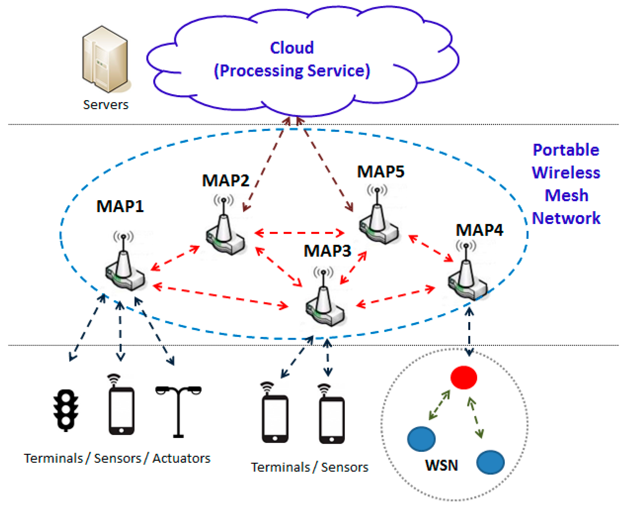
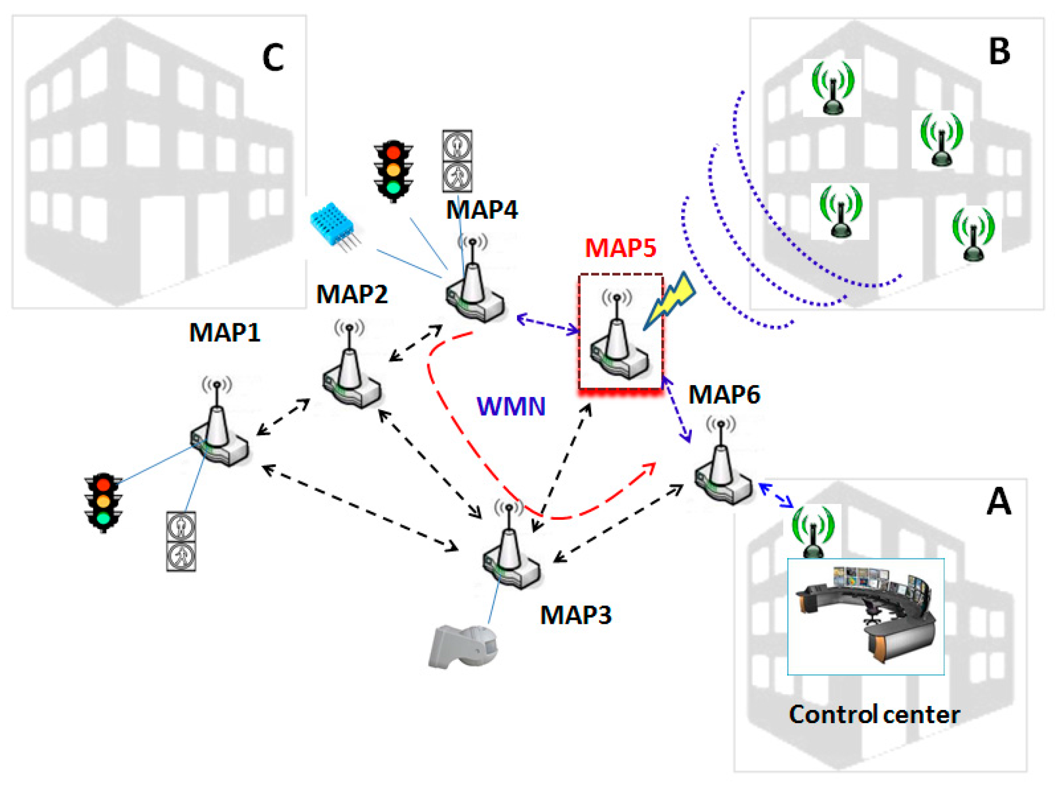
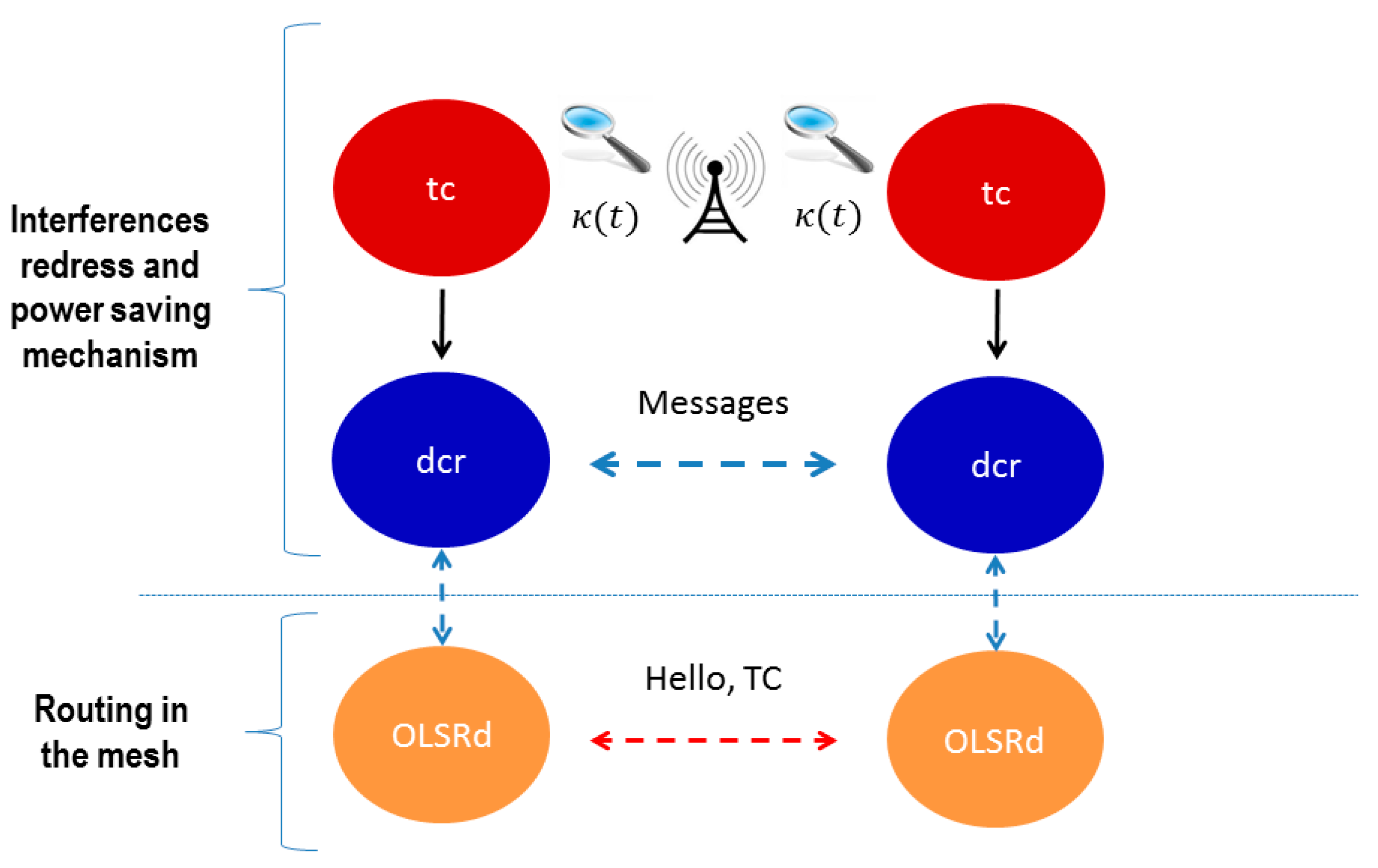
3. System Architecture
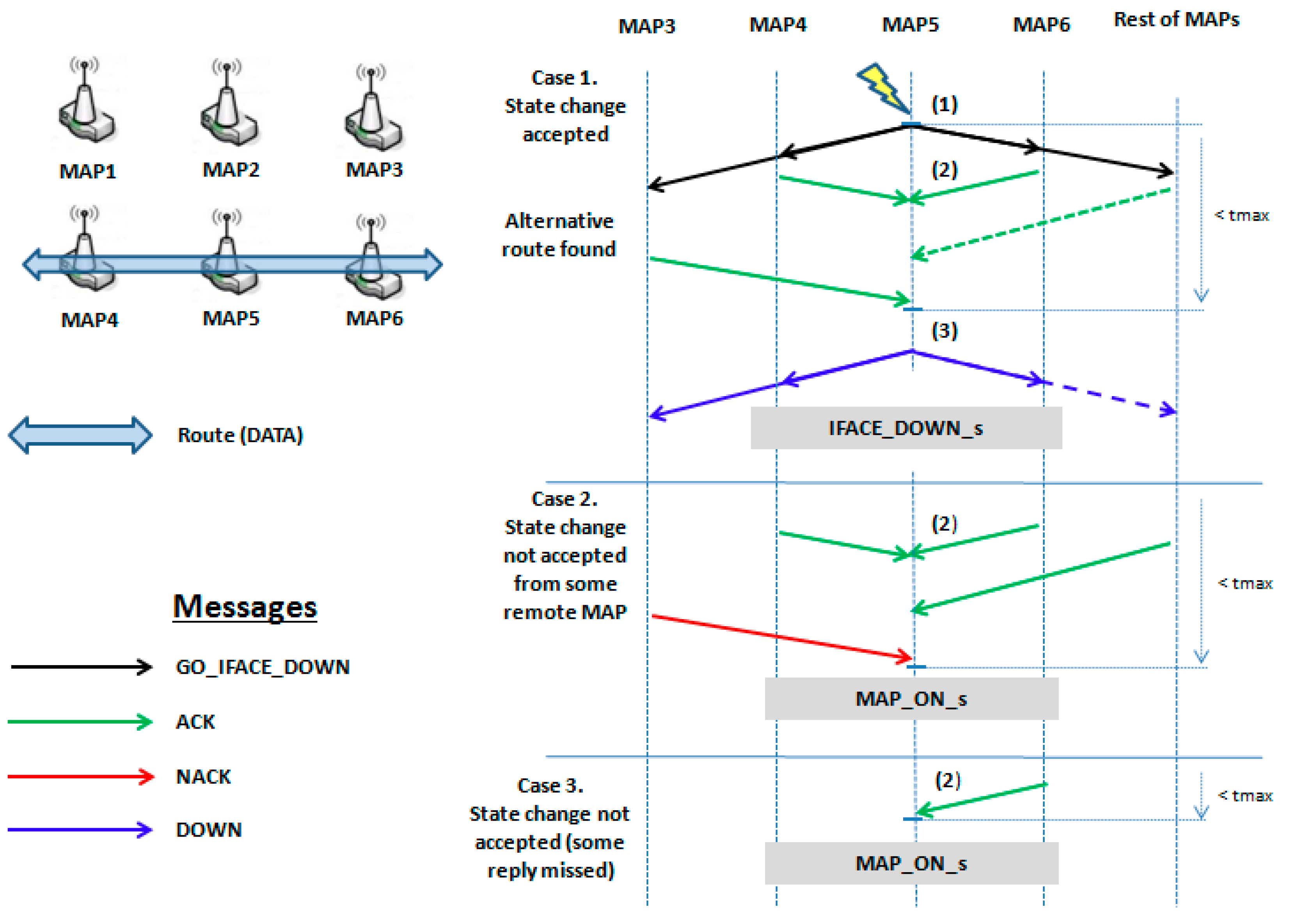
4. The Up/Down Mechanism of WiFi MAPs
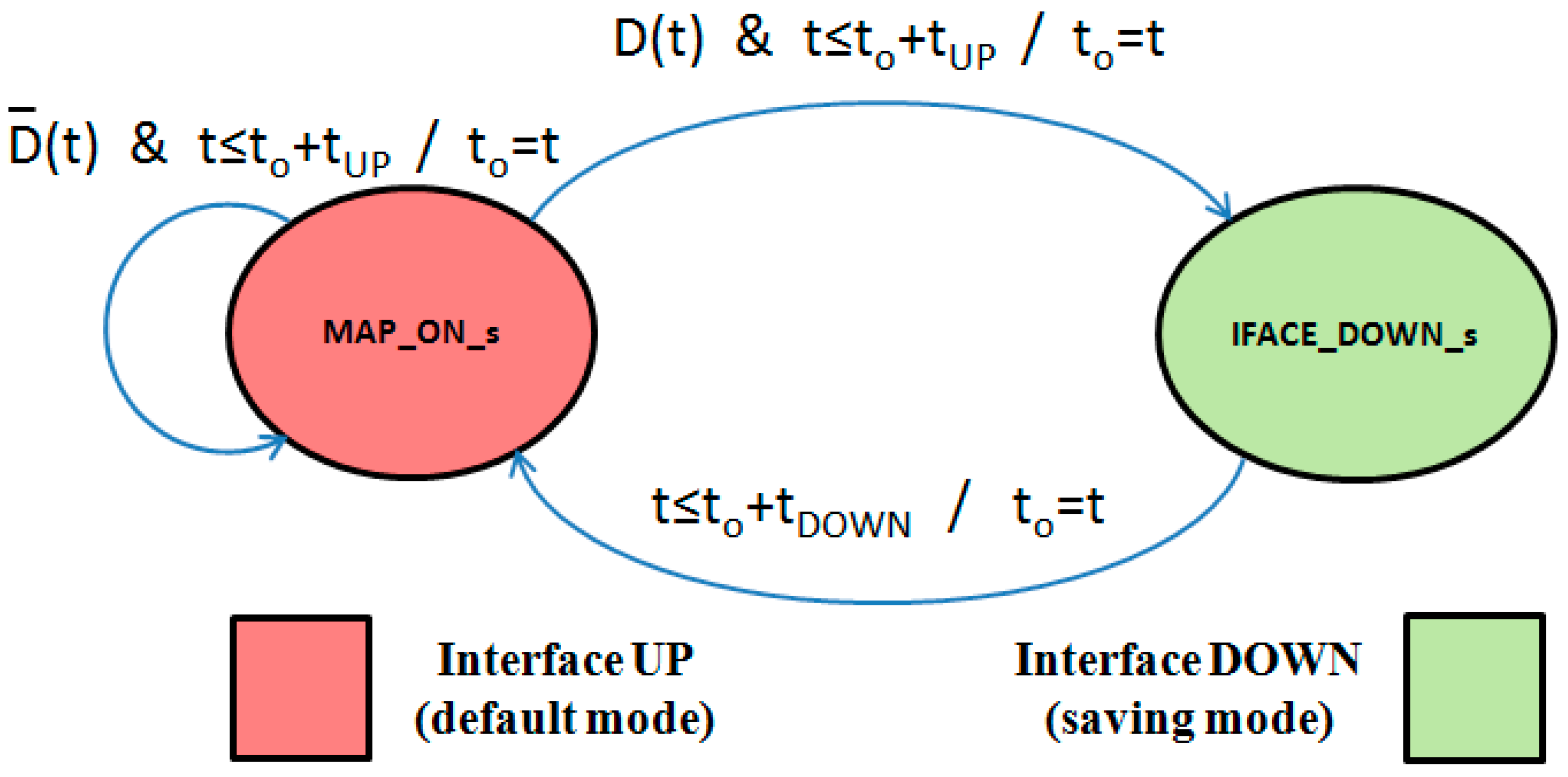
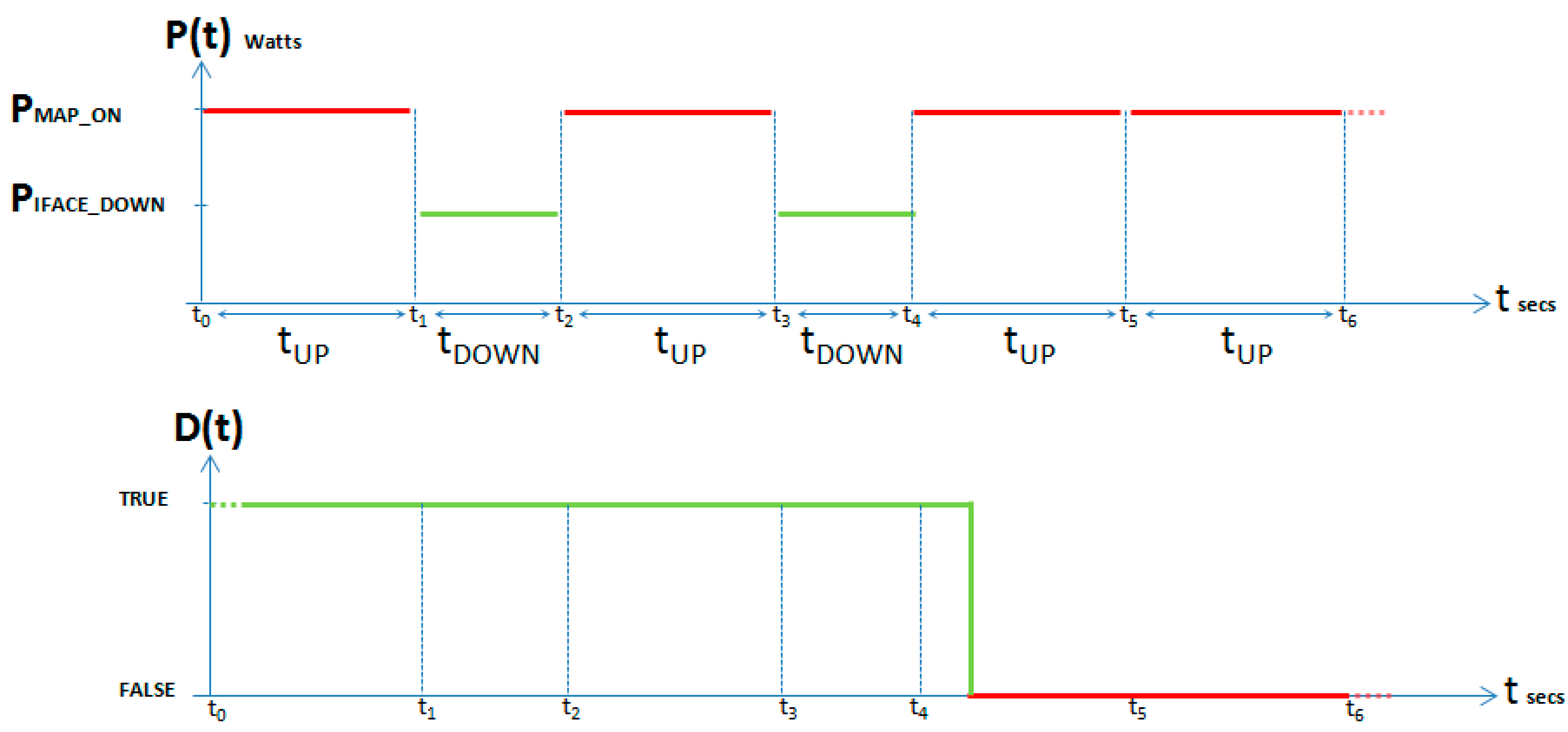
4.1. State Diagram
- 9.4 Watts in MAP_ON_s (i.e., ).
- 7.6 Watts in IFACE_DOWN_s (i.e., ).
- 53.58 kg of carbon dioxide in MAP_ON_s.
- 43.32 kg of carbon dioxide in IFACE_DOWN_s.
4.2. Basic Ideas on Protocol
4.3. Algorithm Specification
| Algorithm 1: Basic Pseudocode of tc |
| 1: Define θ 2: Repeat 3: Sense (κ) 4: if (κ > θ or MAP is unused) then 5: Dp = true 6: else 7: Dp = false 8: endif 9: Send (Dp) to dcr 10: Forever |
| Algorithm 2: Basic Pseudocode of the dcr Main Process |
| 1: Define MAP_state = MAP_ON_s, tUP, tDOWN 2: Repeat 3: Read (t) 4: to = t 5: Switch (MAP_state) 6: case MAP_ON_s: 7: timedThread (to + tUP, dMAP_proc, neighbour_proc) 8: if (D) then 9: set Wireless Interface DOWN 10: MAP_state = IFACE_DOWN_s 11: endif 12: case IFACE_DOWN_s: 13: Wait (to + tDOWN) 14: set Wireless Interface UP 15: MAP_state = MAP_ON_s 16: endSwitch 17: Forever |
| Algorithm 3: Basic Pseudocode of the dcr dMAP_Proc Process |
| timedThread dMAP_proc 1: D = false 2: Receive (Dp) from tc 3: if (Dp) then 4: Send (GO_IFACE_DOWN) to neighbours’ dcr 5: Receive (confirmation, tDOWN, timeout) from neighbours’ dcr 6: if (confirmation = ACK and not timeout) then 7: Send(DOWN) to neighbours’ dcr 8: tDOWN = min(tDOWN received from neighbours’ dcr) 9: D = true 10: endif 11: endif endtimedThread |
| Algorithm 4: Basic Pseudocode of the dcr Neighbour_Proc Process |
| timedThread neighbour_proc 1: Receive (GO_IFACE_DOWN) from id_MAP 2: if (id_MAP is used in a route for any sink and not alternative route for that sink) then 3: Send (NACK) to id_MAP 4: else 5: Evaluate (tDOWN) for id_MAP 6: Send (ACK, tDOWN) to id_MAP 7: endif 8: Receive (confirmation, timeout) from id_MAP 9: if (confirmation = DOWN and not timeout) then 10: UpdateDB (delete any route which includes id_MAP) 11: end endtimedThread |
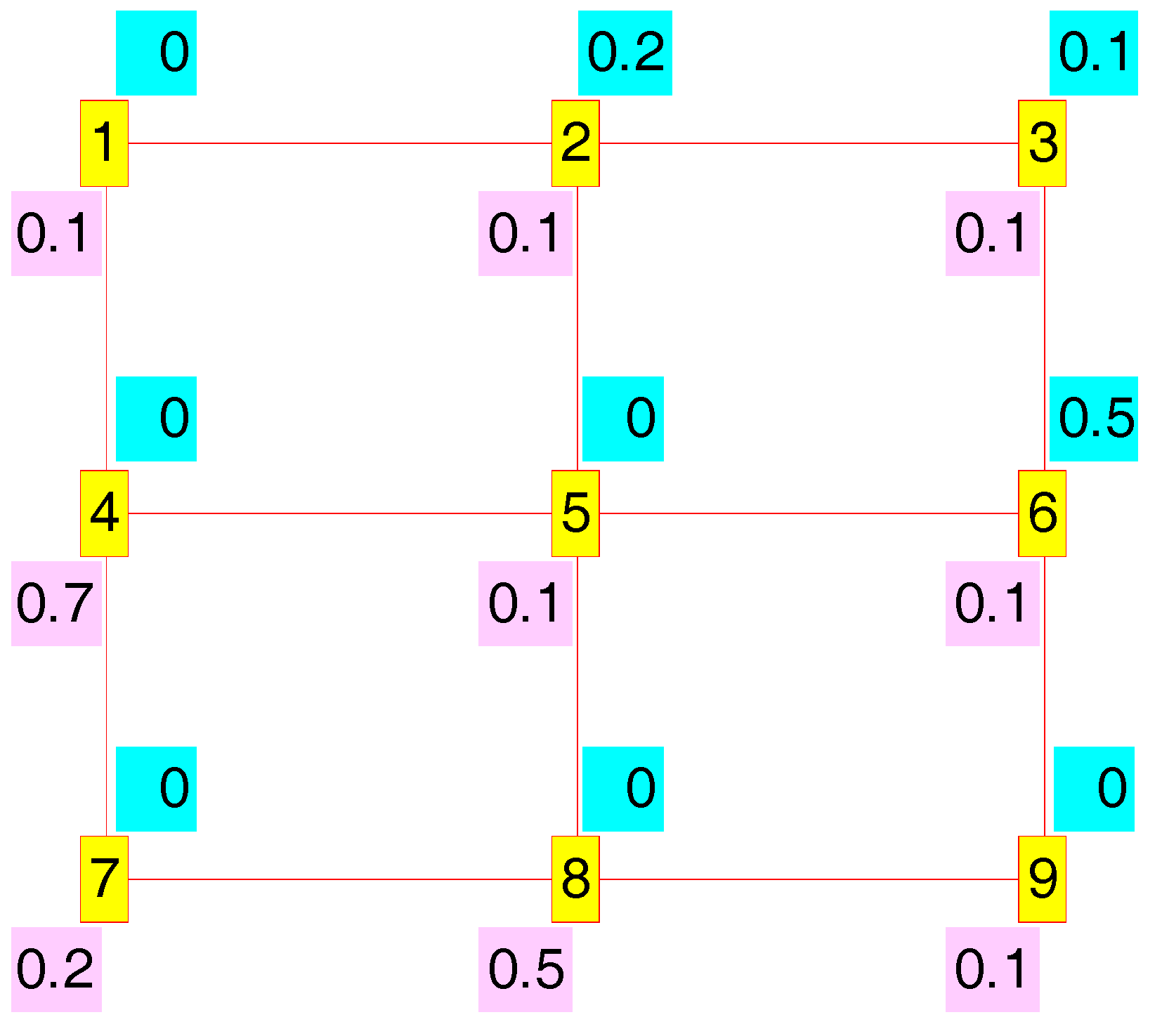
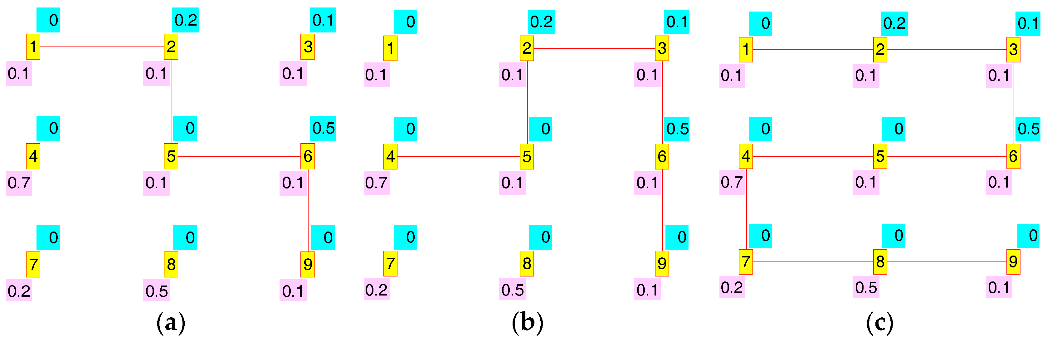
5. Interference Redress and Power Saving Factors
5.1. Mathematical Model
5.2. Simulation Results for Power Saving and Interference Redress Factors
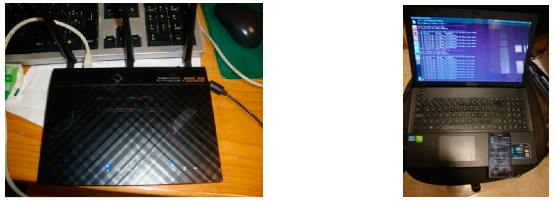
6. Experimental Results for a Test Platform Based on Raspberry Pi
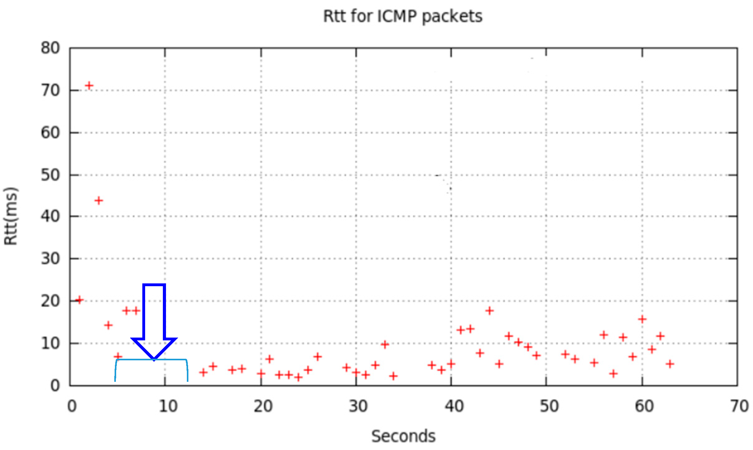
6.1. Interface Deactivation and External Traffic Effects
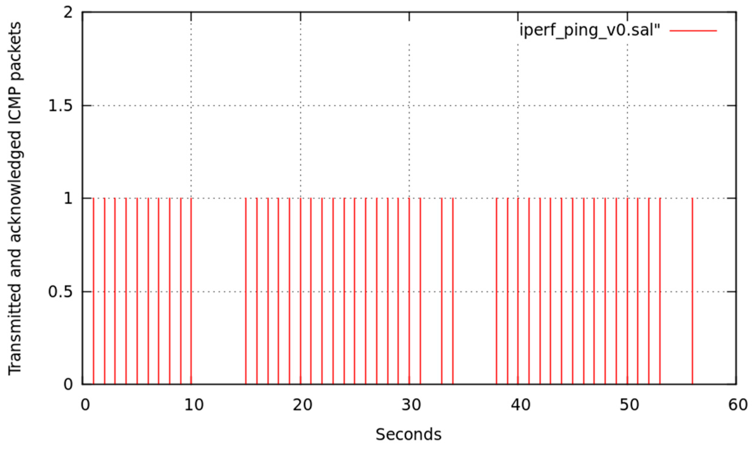
- Connection-less Low Frequency Traffic (LFT) with Internet Control Message Protocol (ICMP).
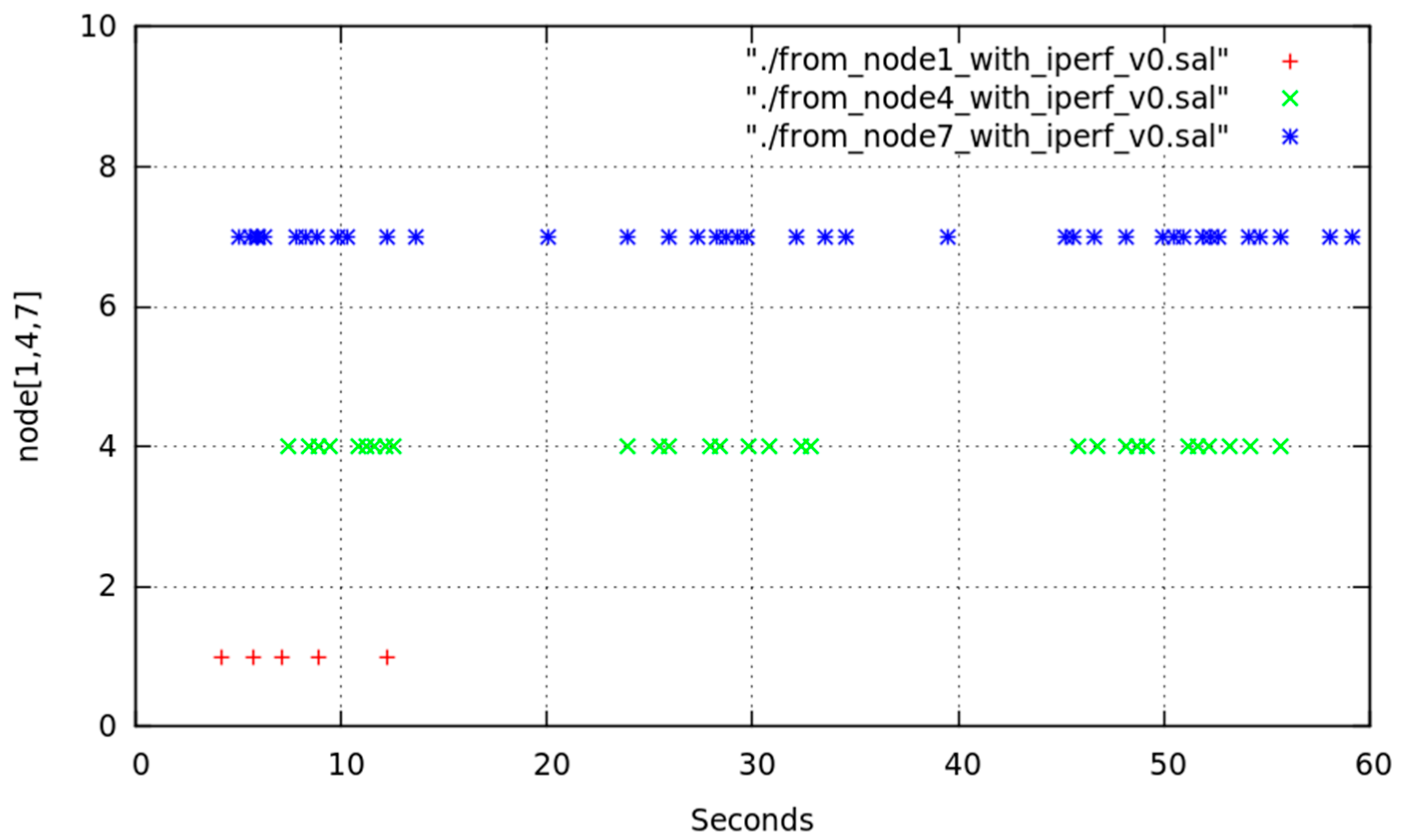
- Connection-oriented High volume and Frequency previously stored Traffic (HFT) with Secure Copy (scp).
6.1.1. Effect of WiFi Interface Deactivation
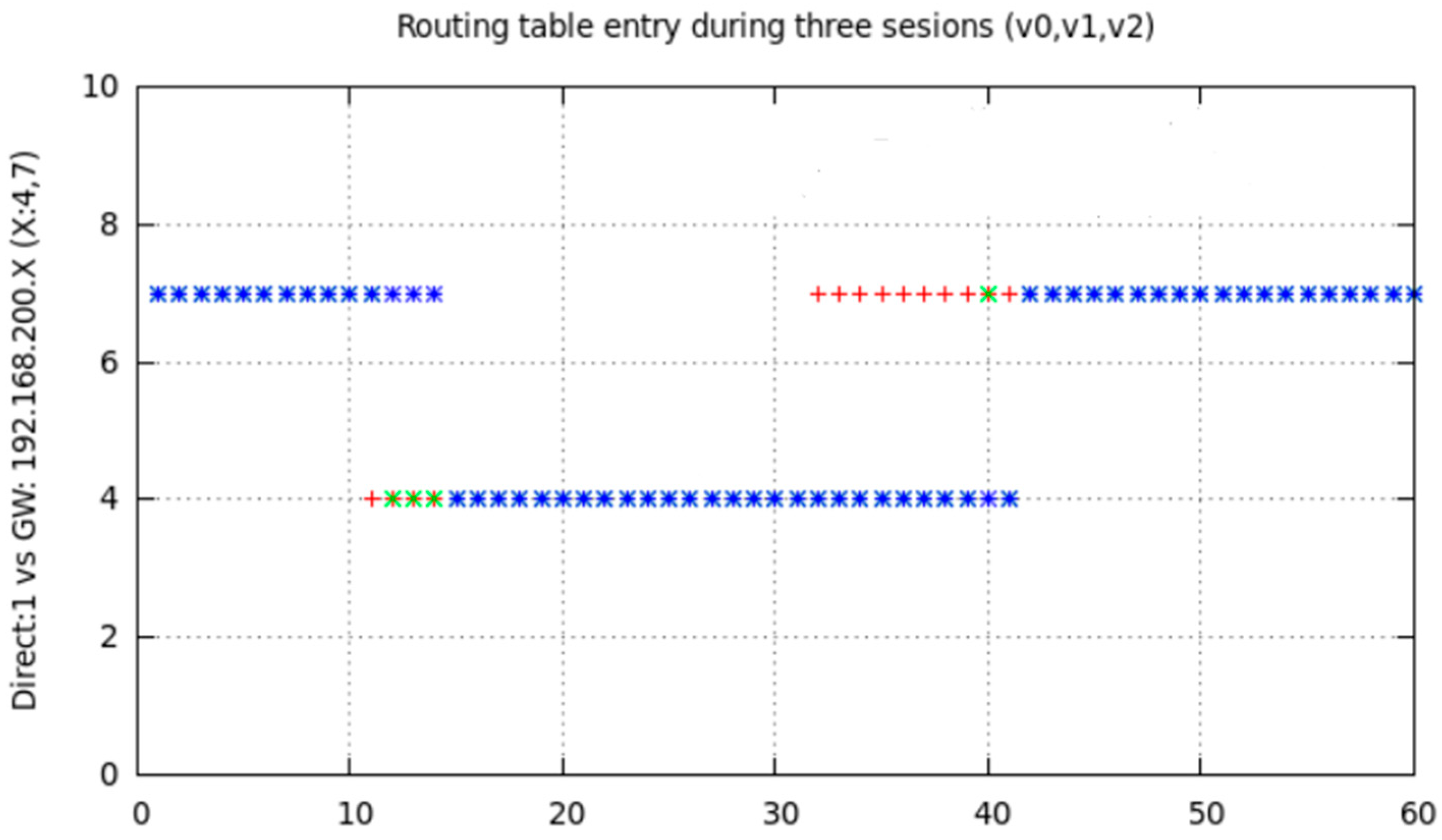
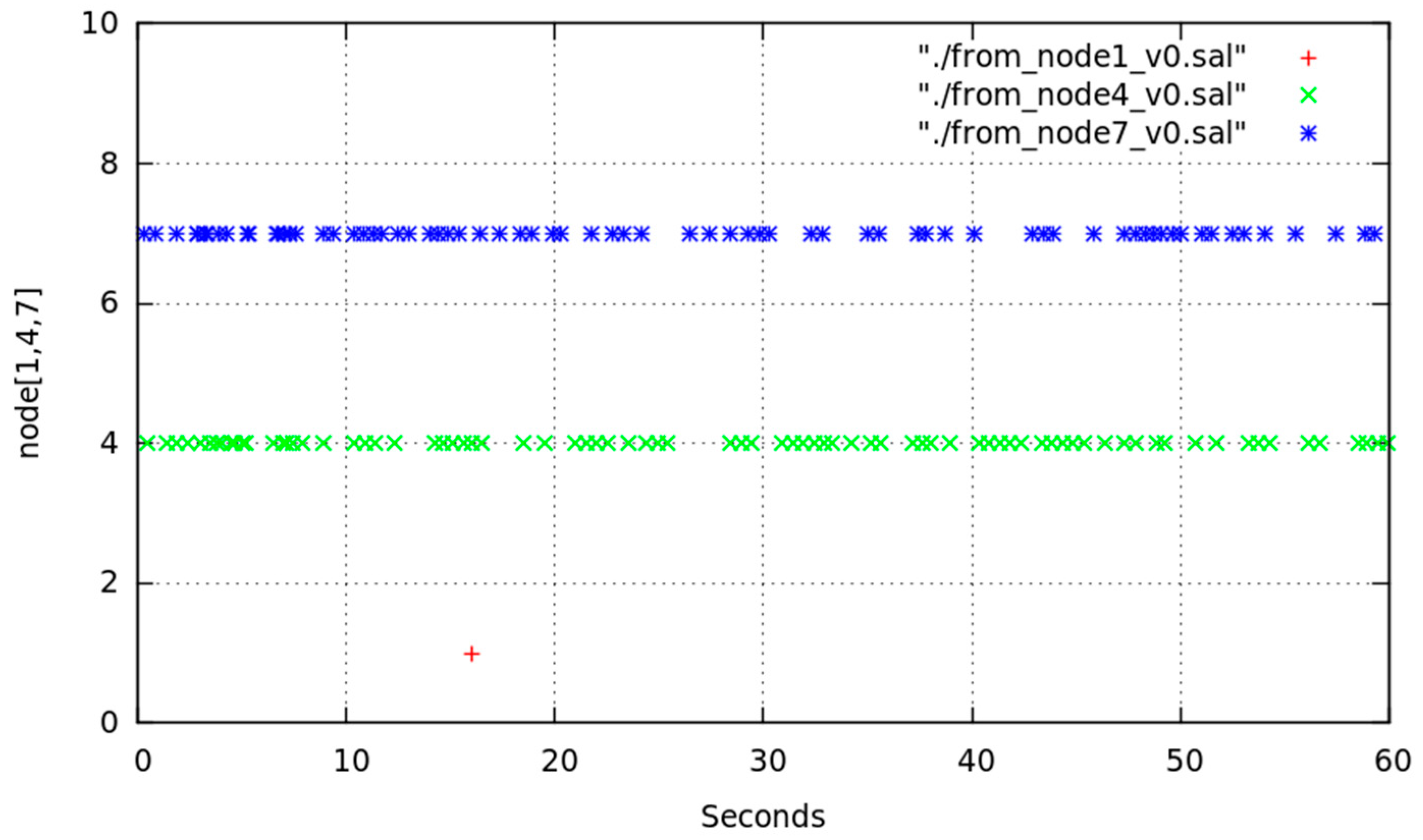
6.1.2. Interference Effects
- (a)
- With very spurious signals on adjacent channels out of our control.
- (b)
- With an AP on channel 11 (which is adjacent to the channel used on the test platform) and emitting only control frames (especially beacons) which we have called Interfering_AP_1.
- (c)
- With an AP on channel 11 and another in channel 7 (same channel as our PWMNS configuration) which we have called Interfering_AP_2.
- (d)
- Interfering_AP_1 and Interfering_AP_2, but the latter transporting intensive user traffic (using iperf [52] application which we consider as interfering traffic for our network).
6.2. Power Saving Calculation
7. Conclusions
Acknowledgments
Author Contributions
Conflicts of Interest
References
- Akyildiz, I.F.; Xudong, W. A survey on wireless mesh networks. IEEE Commun. Mag. 2005, 43, S23–S30. [Google Scholar] [CrossRef]
- Hossain, E.; Leung, K.K. Wireless Mesh Networks; Architectures and Protocols; Springer: New York, NY, USA, 2008. [Google Scholar]
- Lee, M.J.; Jianliang, Z.; Young-Bae, K.; Deepesh Man, S. Emerging standards for wireless mesh technology. IEEE Wirel. Commun. 2006, 13, 56–63. [Google Scholar] [CrossRef]
- Hiertz, G.; Denteneer, D.; Max, S.; Taori, R.; Cardona, J.; Berlemann, L.; Walke, B. IEEE 802.11s: The WLAN mesh standard. IEEE Wirel. Commun. 2010, 17, 104–111. [Google Scholar] [CrossRef]
- Bicket, J.; Aguayo, D.; Biswas, S.; Morris, R. Architecture and Evaluation of an Unplanned 802.11b Mesh Network. In Proceedings of the 11th Annual International Conference on Mobile Computing and Networking, Cologne, Germany, 28 August–2 September 2005; pp. 31–42. [Google Scholar]
- Akyildiz, I.F.; Wang, X.; Wang, W. Wireless mesh networks: A survey. Comput. Netw. 2005, 47, 445–487. [Google Scholar] [CrossRef]
- He, Y.; Stojmenovic, I.; Liu, Y.; Gu, Y. Smart city. Int. J. Distrib. Sens. Netw. 2014, 10. [Google Scholar] [CrossRef]
- Murty, R.N.; Mainland, G.; Rose, I.; Chowdhury, A.R.; Gosain, A.; Bers, J.; Welsh, M. Citysense: An Urban-Scale Wireless Sensor Network and Testbed. In Proceedings of the IEEE Conference on Technologies for Homeland Security, Waltham, MA, USA, 12–13 May 2008; pp. 583–588. [Google Scholar]
- Bruno, R.; Conti, M.; Pinizzotto, A. Routing internet traffic in heterogeneous mesh networks: Analysis and algorithms. Perform. Eval. 2011, 68, 841–858. [Google Scholar] [CrossRef]
- Tang, J.; Xue, G.; Zhang, W. Interference-Aware Topology Control and QoS Routing in Multi-Channel Wireless Mesh Networks. In Proceedings of the 6th ACM International Symposium on Mobile Ad Hoc Networking and Computing, Urbana-Champaign, IL, USA, 25–27 May 2005; pp. 68–77. [Google Scholar]
- Raj, M.; Kant, K.; Das, S.K. E-darwin: Energy Aware Disaster Recovery Network Using WiFi Tethering. In Proceedings of the 23rd International Conference on Computer Communication and Networks, Shanghai, China, 4–7 August 2014; pp. 1–8. [Google Scholar]
- Lee, K.; Lee, J.; Yi, Y.; Rhee, I.; Chong, S. Mobile data offloading: How much can WiFi deliver? IEEE ACM Trans. Netw. 2013, 21, 536–550. [Google Scholar] [CrossRef]
- Campista, M.E.M.; Esposito, P.M.; Moraes, I.M.; Costa, L.H.M.; Duarte, O.C.M.; Passos, D.G.; de Albuquerque, C.V.N.; Saade, D.C.M.; Rubinstein, M.G. Routing metrics and protocols for wireless mesh networks. IEEE Netw. 2008, 22, 6–12. [Google Scholar] [CrossRef]
- Johnson, D.; Hancke, G. Comparison of two routing metrics in OLSR on a grid based mesh network. Ad Hoc Netw. 2009, 7, 374–387. [Google Scholar] [CrossRef]
- Arce, P.; Guerri, J.C.; Pajares, A.; Lázaro, O. Performance evaluation of video streaming over ad hoc networks using flat and hierarchical routing protocols. Mob. Netw. Appl. 2008, 13, 324–336. [Google Scholar] [CrossRef]
- Sarmiento, Á.S.; La-Menza, M.; Macías, E.M.; Sunderam, V.S. Automatic Resumption of Streaming Sessions over Wireless Communications Using Agents. In Proceedings of the International MultiConference of Engineers and Computer Scientists, Hong Kong, China, 20–22 June 2006; pp. 926–931. [Google Scholar]
- De la Oliva, A.; Banchs, A.; Serrano, P. Throughput and energy-aware routing for 802.11 based mesh networks. Comput. Commun. 2012, 35, 1433–1446. [Google Scholar] [CrossRef]
- Conti, M.; Giordano, S. Mobile ad hoc networking: Milestones, challenges, and new research directions. IEEE Commun. Mag. 2014, 52, 85–96. [Google Scholar] [CrossRef]
- Olwal, T.O.; Van Wyk, B.J.; Ntlatlapa, N.; Djouani, K.; Siarry, P.; Hamam, Y. Dynamic power control for wireless backbone mesh networks: A survey. Netw. Protoc. Algorithms 2010, 2. [Google Scholar] [CrossRef]
- Escolar, S.; Carretero, J.; Marinescu, M.-C.; Chessa, S. Estimating energy savings in smart street lighting by using an adaptive control system. Int. J. Distrib. Sens. Netw. 2014, 10, 971587. [Google Scholar] [CrossRef]
- Cellucci, L.; Burattini, C.; Drakou, D.; Gugliermetti, F.; Bisegna, F.; Vollaro, A.; Salata, F.; Golasi, I. Urban lighting project for a small town: Comparing citizens and authority benefits. Sustainability 2015, 7, 14230–14244. [Google Scholar] [CrossRef]
- Rodríguez-Molina, J.; Martínez, J.-F.; Castillejo, P.; de Diego, R. Smarc: A proposal for a smart, semantic middleware architecture focused on smart city energy management. Int. J. Distrib. Sens. Netw. 2013, 9, 1–17. [Google Scholar] [CrossRef]
- Li, Q.; Yang, P. Ecots: Efficient and cooperative task sharing for large-scale smart city sensing application. Int. J. Distrib. Sens. Netw. 2014, 2014, 1–14. [Google Scholar] [CrossRef]
- Ha, R.W.; Ho, P.H.; Shen, X. Optimal sleep scheduling with transmission range assignment in application-specific wireless sensor networks. Int. J. Distrib. Sens. Netw. 2006, 1, 72. [Google Scholar] [CrossRef]
- Marrero, D.; Macías, E.; Suárez, Á.; Santana, J.A.; Mena, V. A method for power saving in dense WiFi networks. Mob. Netw. Appl. 2016, 1–12. [Google Scholar] [CrossRef]
- Marrero, D.; Macías, E.; Suárez, Á.; Santana, J.A.; Mena, V. Energy saving in smart city wireless backbone network for environment sensors. Mob. Netw. Appl. 2016, 1–12. [Google Scholar] [CrossRef]
- Khatoun, R.; Zeadally, S. Smart cities: Concepts, architectures, research opportunities. Commun. ACM 2016, 59, 46–57. [Google Scholar] [CrossRef]
- Raspberri Pi Documentation. Available online: https://www.raspberrypi.org/documentation/ (accessed on 24 April 2017).
- Van Der Schaar, M.; Sai Shankar, N. Cross-layer wireless multimedia transmission: Challenges, principles, and new paradigms. IEEE Wirel. Commun. 2005, 12, 50–58. [Google Scholar] [CrossRef]
- Macías, E.; Suárez, A.; Martín, J.; Sunderam, V. Using olsr for streaming video in 802.11 ad hoc networks to save bandwidth. IAENG Int. J. Comput. Sci. 2007, 33, 101–110. [Google Scholar]
- Clausen, T.; Jacquet, P. Optimized Link State Routing Protocol (OLSR). Available online: https://tools.ietf.org/html/rfc3626 (accessed on 24 April 2017).
- Arce Vila, P. Hierarchical Routing and Cross-Layer Mechanisms for Improving Video Streaming Quality of Service Over Mobile Wireless Ad Hoc Networks. Ph.D. Thesis, Universitat Politècnica de València, València, Spain, 2014. [Google Scholar]
- Kanchanasut, K.; Tunpan, A.; Awal, M.; Wongsaardsakul, T.; Das, D.; Tsuchimoto, Y. Building a Long-Distance Multimedia Wireless Mesh Network for Collaborative Disaster Emergency Responses; Internet Education and Research Laboratory: Pathum Thani, Thailand, 2007. [Google Scholar]
- Sun, W.; Wang, H.; Piao, X.; Qiu, T. An opportunistic routing mechanism combined with long-term and short-term metrics for WMN. Sci. World J. 2014, 2014, 11. [Google Scholar] [CrossRef] [PubMed]
- Serrano, S.; Campobello, G.; Leonardi, A.; Palazzo, S.; Galluccio, L. VoIP traffic in wireless mesh networks: A MOS-based routing scheme. Wirel. Commun. Mob. Comput. 2016, 16, 1192–1208. [Google Scholar] [CrossRef]
- Li, Z.; Wang, H.; Dong, C.; Qian, R. Urp: A Unified Routing Protocol for Heterogeneous Wireless Mesh Networks. In Proceedings of the IEEE Wireless Communications and Networking Conference, Shanghai, China, 7–10 April 2013; pp. 2255–2260. [Google Scholar]
- Li, Z.; Wang, H.; Dong, C.; Wu, F.; Yu, W. Unified routing protocol based on passive bandwidth measurement in heterogeneous WMNs. Wirel. Commun. Mob. Comput. 2016, 16, 2356–2373. [Google Scholar] [CrossRef]
- Rigelsford, J.; Ford, K.; Yu, T.; Lai, Z.; Valtr, P.; Weng, J.; Wang, Y.; Vallecchi, A.; Altan, H.; Song, H. Wireless Friendly and Energy Efficient Buildings (WiFEEB). In Proceedings of the Progress in Electromagnetics Research Symposium Abstracts, Prague, Czech Republic, 6–9 July 2015. [Google Scholar]
- Alotaibi, E.; Mukherjee, B. A survey on routing algorithms for wireless ad-hoc and mesh networks. Comput. Netw. 2012, 56, 940–965. [Google Scholar] [CrossRef]
- Vijayakumar, K.; Ganeshkumar, P.; Anandaraj, M. Review on routing algorithms in wireless mesh networks. Int. J. Comput. Sci. Telecommun. 2012, 3, 87–92. [Google Scholar]
- Ahmeda, S.S.; Farhan, R.K. Routing protocols for wireless mesh networks. In Proceedings of the 1st International Congress on Computer, Electronics, Electrical, and Communication Engineering, Chennai, India, 17–18 March 2014; pp. 142–148. [Google Scholar]
- Marrero, D.; Macías, E.M.; Suárez, A. An admission control and traffic regulation mechanism for infrastructure WiFi networks. IAENG Int. J. Comput. Sci. 2008, 35, 154–160. [Google Scholar]
- Dely, P.; D’Andreagiovanni, F.; Kassler, A. Fair optimization of mesh-connected WLAN hotspots. Wirel. Commun. Mob. Comput. 2015, 15, 924–946. [Google Scholar] [CrossRef]
- Nandiraju, N.; Nandiraju, D.; Agrawal, D. Multipath Routing in Wireless Mesh Networks. In Proceedings of the IEEE International Conference on Mobile Adhoc and Sensor Systems, Vancouver, BC, Canada, 9–12 October 2006; pp. 741–746. [Google Scholar]
- Wireless-g Broadband Router. Available online: http://www.linksys.com/us/support-product?pid=01t80000003KXPxAAO (accessed on 24 April 2017).
- Unleash Your Router. Available online: http://www.dd-wrt.com/site/index (accessed on 24 April 2017).
- Calculator for Consumption in Standby. Available online: http://www.ocu.org/vivienda-y-energia/nc/calculadora/consumo-en-stand-by (accessed on 24 April 2017).
- Linksys Official Support—Linksys WRT160NL Wireless-N Broadband Router with Storage Link. Available online: http://www.linksys.com/us/support-product?pid=01t80000003K7eJAAS (accessed on 24 April 2017).
- Marrero Marrero, D. Characterizing and Modelling Wireless Network Performance for Applications with Quality of Service. Ph.D. Thesis, University of Las Palmas de Gran Canaria, Gran Canaria, Spain, 2016. (In Spanish). [Google Scholar]
- Santana, J.A.; Macías, E.; Suárez, Á.; Marrero, D.; Mena, V. Adaptive estimation of WiFi RSSI and its impact over advanced wireless services. Mob. Netw. Appl. 2016. [Google Scholar] [CrossRef]
- Lakshminarayanan, K.; Seshan, S.; Steenkiste, P. Understanding 802.11 performance in heterogeneous environments. In Proceedings of the 2nd ACM SIGCOMM Workshop on Home networks, Toronto, ON, Canada, 15–19 August 2011; pp. 43–48. [Google Scholar]
- iPerf—The Ultimate Speed Test Tool for TCP, UDP and SCTP. Available online: https://iperf.fr/ (accessed on 24 April 2017).


| State Name | MAP Wireless Interface Is | Full MAP System Is |
|---|---|---|
| MAP_OFF_s | down | off (it does consume no power) |
| IFACE_DOWN_s | down | on and its wireless interface is down |
| MAP_ON_s | up | on and its wireless interface is up |
| State Name | Bandwidth | Power (Watts) |
|---|---|---|
| MAP_ON_s (b, g or n) | 20 MHz | 3.5 |
| MAP_ON_s (n version only) | 40 MHz | 4.4 |
| IFACE_DOWN_s | any | 2.8 |
| Message Name | Arguments | Direction | Description |
|---|---|---|---|
| GO_IFACE_DOWN | tDOWN, id_MAP | dMAP → neighbours | MAP is downable |
| ACK | tDOWN, id_MAP | neighbours → dMAP | Neighbour accept dMAP change to IFACE_DOWN_s |
| NACK | Motive (reason for refusal) | neighbours → dMAP | Neighbour refuse dMAP change to IFACE_DOWN_s |
| DOWN | dMAP → neighbours | End of negotiation |
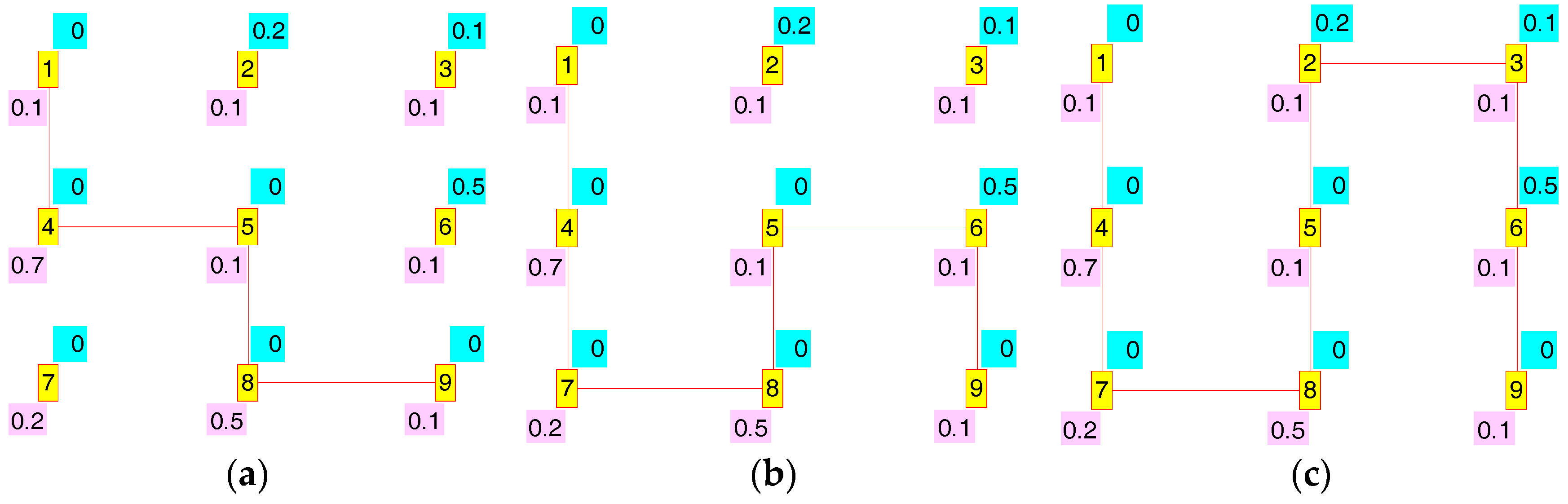
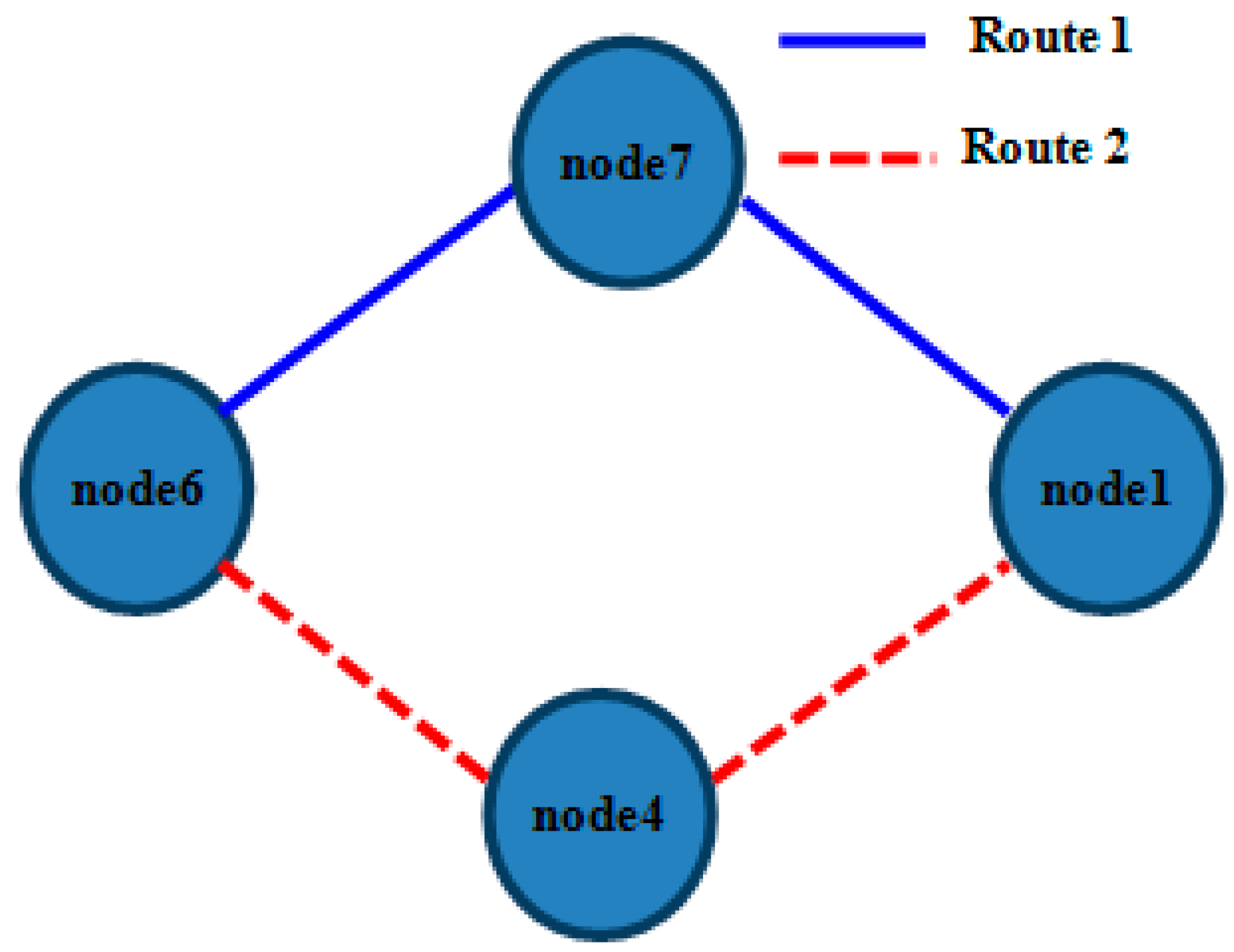
| Route | R(t) | S(t) | ||
|---|---|---|---|---|
| 1-4-5-8-9 | 1 | 0 | 0.3 | 1.5 |
| 1-4-7-8-9 | 1 | 0 | 0.3 | 1.6 |
| 1-2-5-8-9 | 0.8 | 0.2 | 0.7 | 0.9 |
| 1-2-5-4-7-8-9 | 0.8 | 0.2 | 0.1 | 1.8 |
| 1-4-5-6-9 | 0.4 | 0.5 | 0.6 | 1.1 |
| 1-4-7-8-5-6-9 | 0.4 | 0.5 | 0.1 | 1.8 |
| 1-2-5-6-9 | 0.1 | 0.7 | 1 | 0.5 |
| 1-2-3-6-9 | 0 | 0.8 | 1 | 0.5 |
| 1-2-3-6-5-8-9 | 0 | 0.8 | 0.6 | 1.1 |
| 1-4-5-2-3-6-9 | 0 | 0.8 | 0.5 | 1.3 |
| 1-2-3-6-5-4-7-8-9 | 0 | 0.8 | 0 | 2 |
| 1-4-7-8-5-2-3-6-9 | 0 | 0.8 | 0 | 2 |
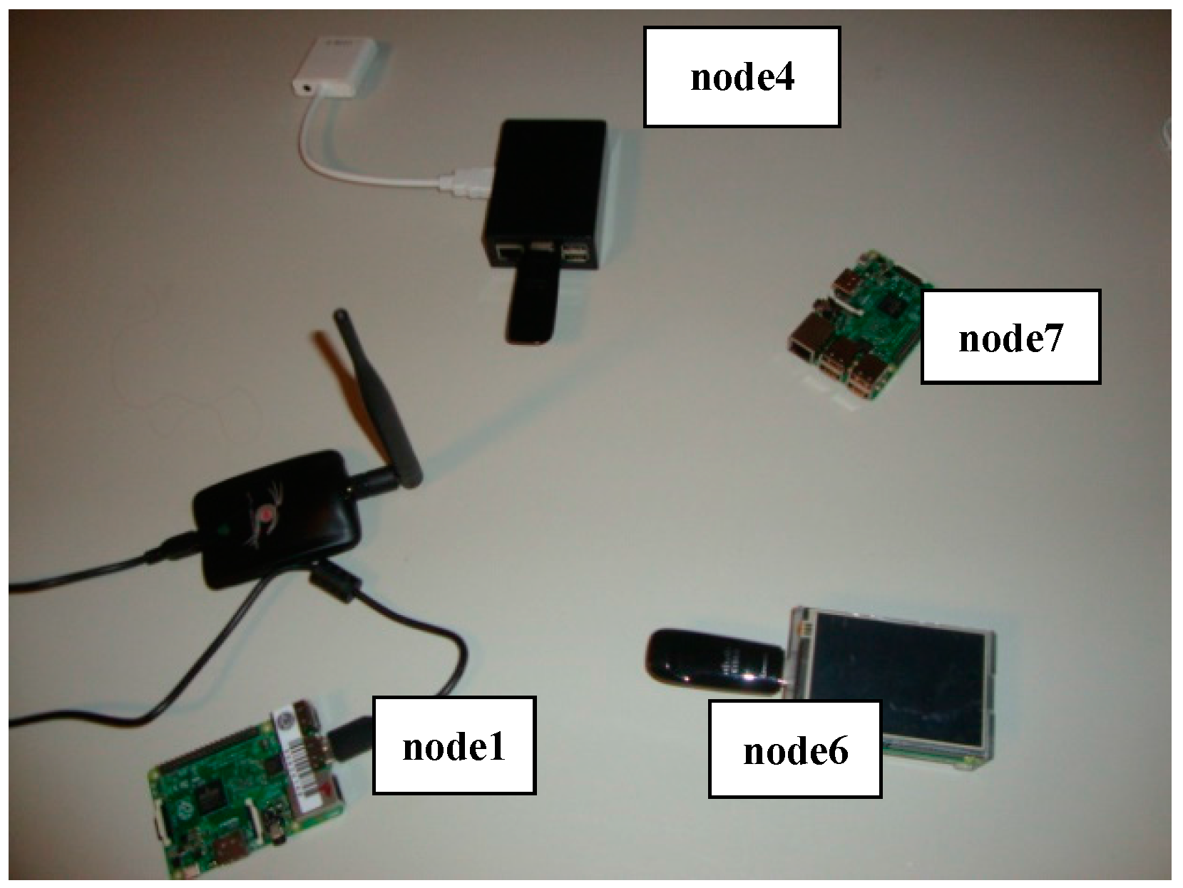
| node4 | RPi2: WiFi Linksys Cisco WUSB600N interface, Debian RPi kernel ver. 4.1.17-v7+ |
| node1 | RPi2: Alfa Chipset Realtek 8187L interface and 6 dBi antenna, Debian RPi kernel ver. 4.1.17-v7+ |
| node6 | RPi2+: Display LCD with WiFi Linksys Cisco WUSB600N interface, Debian RPi kernel ver. 4.1.17-v7+ |
| node7 | RPi3: internal WiFi interface Raspbian Jessie kernel ver. 4.4 (11 January 2017) |
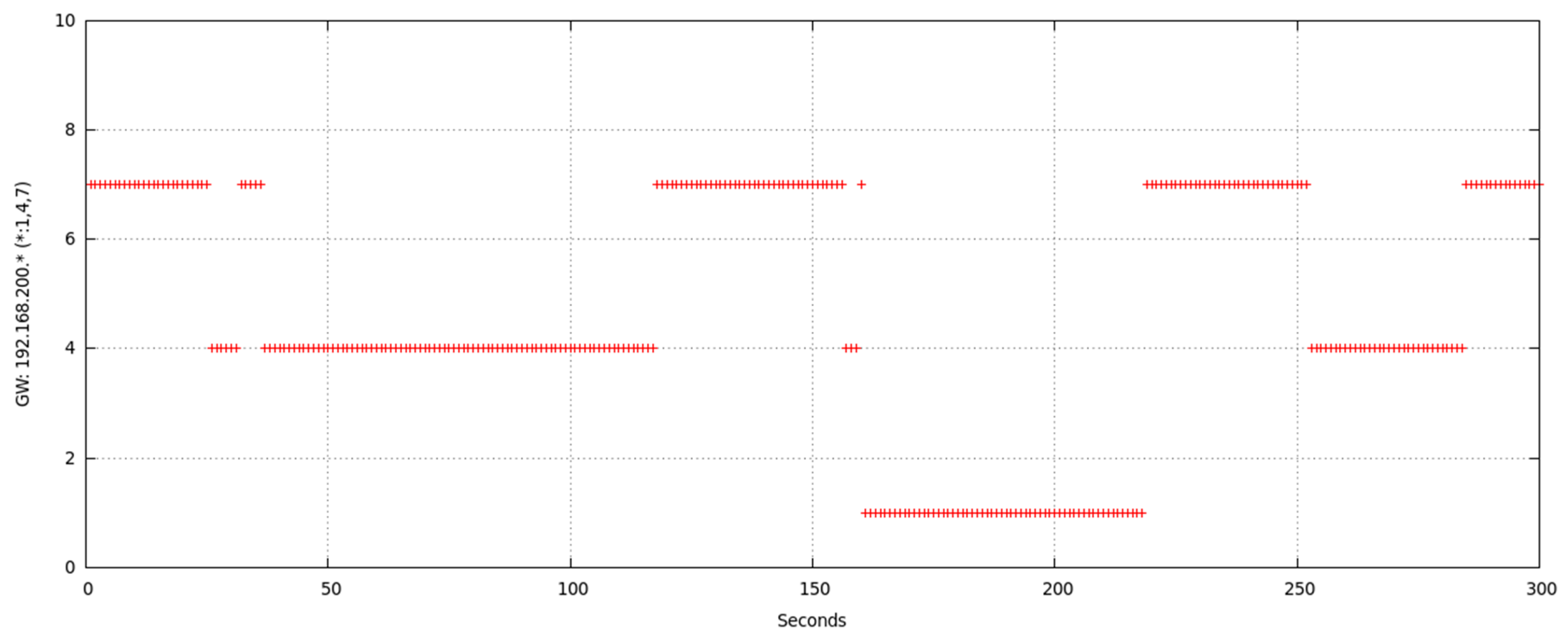
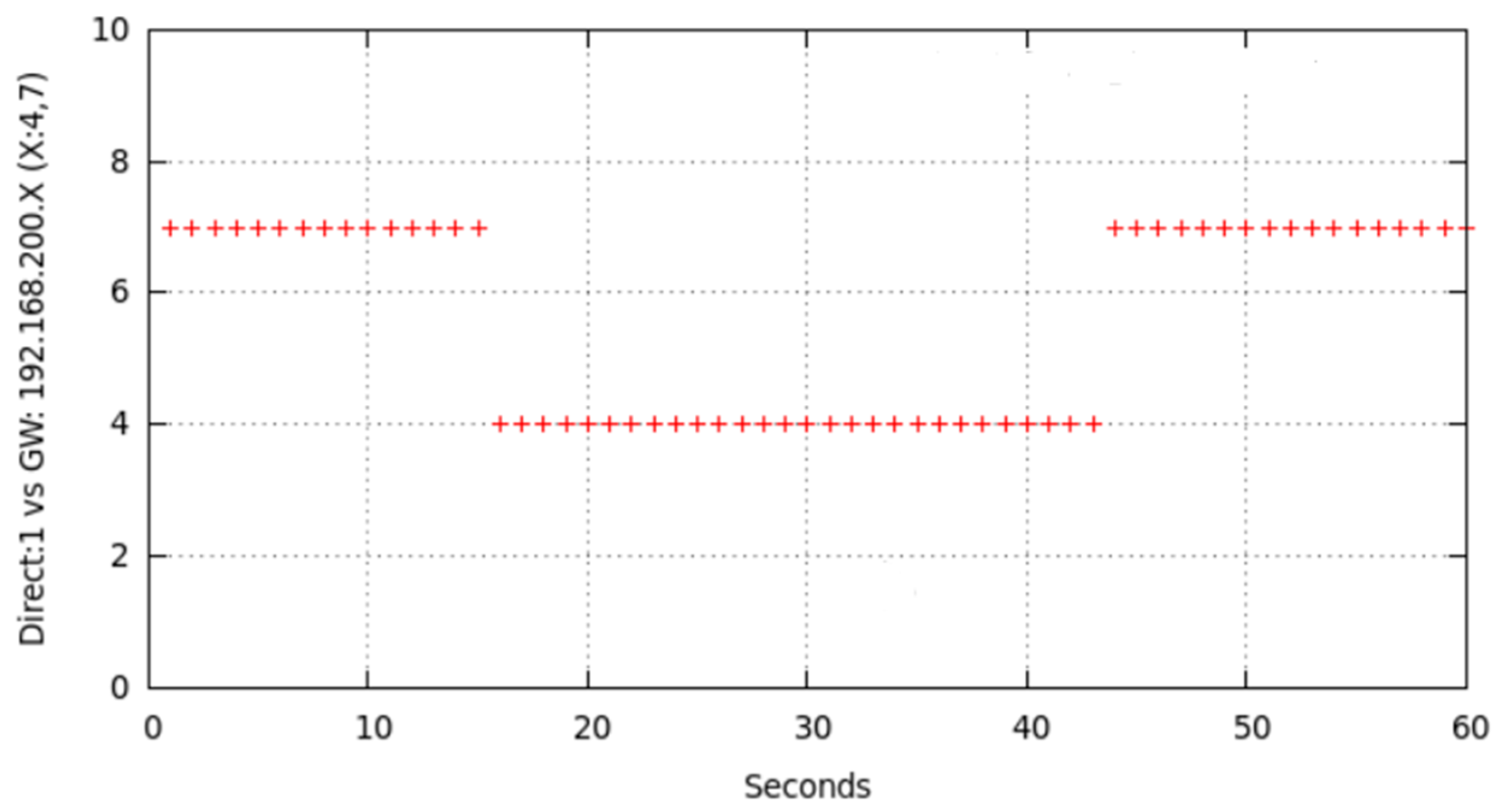
| Destination | Gateway | Genmask | Flags | Metric | Ref | Use IFace |
|---|---|---|---|---|---|---|
| 169.254.0.0 | 0.0.0.0 | 255.255.0.0 | U | 303 | 0 | 0 wlan0 |
| 192.168.200.0 | 0.0.0.0 | 255.255.255.0 | U | 0 | 0 | 0 wlan0 |
| 192.168.200.1 | 192.168.200.7 | 255.255.255.255 | UGH | 2 | 0 | 0 wlan0 |
| 192.168.200.4 | 192.168.200.4 | 255.255.255.255 | UGH | 2 | 0 | 0 wlan0 |
| 192.168.200.7 | 192.168.200.7 | 255.255.255.255 | UGH | 2 | 0 | 0 wlan0 |
| pi@raspberrypi:~$ scp/home/pi/temporal.tar [email protected]:/home/pi/temporal.tar | |||
| [email protected]’s password: | |||
| temporal.tar | 100% | 13 MB 207.5 KB/s | 01:05 |
| pi@raspberrypi:~$ scp /home/pi/temporal.tar [email protected]:/home/pi/temporal.tar | |||
| [email protected]’s password: | |||
| temporal.tar | 100% | 13 MB 245.3 KB/s | 00:55 |
| pi@raspberrypi:~$ scp /home/pi/temporal.tar [email protected]:/home/pi/temporal.tar | |||
| [email protected]’s password: | |||
| temporal.tar | 100% | 13 MB 236.7 KB/s | 00:57 |
| ModelIFaces | Without WiFi | Internal | WUSB600N | ALFA | |||
|---|---|---|---|---|---|---|---|
| Down | Up | Down | Up | Down | Up | ||
| RPI3 (node7) | - | 2.0 W | 2.7 W | - | - | - | - |
| RPI2 (node4, node1) | 2 W | - | - | 2.2 W | 3.9 W | 2.9 W | 4.3 W |
| RPI2+LCD (node6) | 3.4 W | - | - | 3.2W (5.9 W) * | 4.4 W (6.2 W) * | - | - |
| node4 | Average_powerT = 3.9 W × tUP + 2.2 W × tDOWN |
| node1 | Average_powerT = 4.3 W × tUP + 2.9 W × tDOWN |
| node6 | Average_powerT = 4.4 W × tUP + 3.2 W × tDOWN |
| node7 | Average_powerT = 2.7 W × tUP + 2.0 W × tDOWN |
| Always MAP_ON_s | IFACE_DOWN_s-MAP_ON_s | |
|---|---|---|
| node4 | 3.9 × 60 = 234 W-min | 3.9 × 45 + 2.2 × 15 = 175.5 + 33 = 208.5 W-min |
| node1 | 4.3 × 60 = 258 W-min | 4.3 × 45 + 2.9 × 15 = 193.5 + 43.5 = 237 W-min |
| node6 | 4.4 × 60 = 264 W-min | 4.4 × 45 + 3.2 × 15 = 198 + 48 = 246 W-min |
| node7 | 2.7 × 60 = 162 W-min | 2.7 × 45 + 2.0 × 15 = 121.2 + 30 = 151.2 W-min |
| Total (1 min) | 918 W-min | 842.7 W-min |
| Total (Watt-hour) | 55.080 kWh | 50.062 kWh |
© 2017 by the authors. Licensee MDPI, Basel, Switzerland. This article is an open access article distributed under the terms and conditions of the Creative Commons Attribution (CC BY) license (http://creativecommons.org/licenses/by/4.0/).
Share and Cite
Santana, J.; Marrero, D.; Macías, E.; Mena, V.; Suárez, Á. Interference Effects Redress over Power-Efficient Wireless-Friendly Mesh Networks for Ubiquitous Sensor Communications across Smart Cities. Sensors 2017, 17, 1678. https://doi.org/10.3390/s17071678
Santana J, Marrero D, Macías E, Mena V, Suárez Á. Interference Effects Redress over Power-Efficient Wireless-Friendly Mesh Networks for Ubiquitous Sensor Communications across Smart Cities. Sensors. 2017; 17(7):1678. https://doi.org/10.3390/s17071678
Chicago/Turabian StyleSantana, Jose, Domingo Marrero, Elsa Macías, Vicente Mena, and Álvaro Suárez. 2017. "Interference Effects Redress over Power-Efficient Wireless-Friendly Mesh Networks for Ubiquitous Sensor Communications across Smart Cities" Sensors 17, no. 7: 1678. https://doi.org/10.3390/s17071678