Synergetic Use of Sentinel-1 and Sentinel-2 Data for Soil Moisture Mapping at 100 m Resolution


1
CESBIO (CNRS/CNES/UPS/IRD), 18 av. Edouard Belin, bpi 2801, 31401 Toulouse CEDEX9, France
2
isardSAT, Parc Tecnològic Barcelona Activa, Carrer de Marie Curie, 8, 08042 Barcelona, Spain
3
Observatori de l’Ebre (OE), Ramon Llull University, C.\ Horta Alta, 38, 43520 Roquetes, Spain
4
IRSTEA, UMR TETIS, 500 rue Franois Breton, 34093 Montpellier CEDEX 5, France
*
Author to whom correspondence should be addressed.
Sensors 2017, 17(9), 1966; https://doi.org/10.3390/s17091966
Submission received: 10 July 2017
/
Revised: 11 August 2017
/
Accepted: 22 August 2017
/
Published: 26 August 2017
(This article belongs to the Special Issue Recent Innovative Microwave Remote Sensing Instrumentation for Land Surface Applications)
Abstract
:The recent deployment of ESA’s Sentinel operational satellites has established a new paradigm for remote sensing applications. In this context, Sentinel-1 radar images have made it possible to retrieve surface soil moisture with a high spatial and temporal resolution. This paper presents two methodologies for the retrieval of soil moisture from remotely-sensed SAR images, with a spatial resolution of 100 m. These algorithms are based on the interpretation of Sentinel-1 data recorded in the VV polarization, which is combined with Sentinel-2 optical data for the analysis of vegetation effects over a site in Urgell (Catalunya, Spain). The first algorithm has already been applied to observations in West Africa by Zribi et al., 2008, using low spatial resolution ERS scatterometer data, and is based on change detection approach. In the present study, this approach is applied to Sentinel-1 data and optimizes the inversion process by taking advantage of the high repeat frequency of the Sentinel observations. The second algorithm relies on a new method, based on the difference between backscattered Sentinel-1 radar signals observed on two consecutive days, expressed as a function of NDVI optical index. Both methods are applied to almost 1.5 years of satellite data (July 2015–November 2016), and are validated using field data acquired at a study site. This leads to an RMS error in volumetric moisture of approximately 0.087 m3/m3 and 0.059 m3/m3 for the first and second methods, respectively. No site calibrations are needed with these techniques, and they can be applied to any vegetation-covered area for which time series of SAR data have been recorded.
1. Introduction
Surface soil moisture plays an essential role in numerous environmental studies related to hydrology, meteorology and agriculture. For hydrological and agricultural applications, accurate soil moisture estimations are essential, since the hydric state of the soil is a key variable in the rainfall-runoff process [1]. Regular evaluation of this parameter can significantly improve flood and drought estimations [2], since it affects the amount of water available for vegetation growth [3,4]. In situ networks represent single point locations, and usually cover relatively short periods of observation [5], whereas the acquisitions of satellite data make it possible to continuously retrieve surface soil moisture, at regional and global scales. Various approaches have been developed for the retrieval of soil moisture, using optical, thermal infrared (TIR), and microwave (MW) sensors [6,7]. Optical sensors in the thermal spectrum are able to identify temperature differences, which can be related to surface soil moisture. Microwave soil moisture estimations are based on the strong contrast between the dielectric properties of water (≈80) and dry soil (<5) [8]. The depth at which the moisture is sensed depends on the sensor frequency but usually does not exceed several centimeters, in order to access rootzone soil moisture a more or less complex model is needed and several approaches have been developed such as techniques based on the energy balance approach based on thermal infrared soil moisture [9] or simplified water balanced approaches [10,11].
Traditional passive remote sensing instruments can be used to determine the surface soil moisture with a temporal resolution of 2–3 days. However, these instruments, which include the European Space Agency (ESA) Soil Moisture and Ocean Salinity (SMOS) mission [12,13] and the National Aeronautics and Space Administration (NASA) Soil Moisture Active Passive (SMAP) mission [14], have a low spatial resolution (around 40 km [15]). With the current Sentinel-1 mission, the active onboard C-band sensor offers regular temporal coverage (about five days for Europe when both A and B satellites are considered), together with a spatial resolution of 10 m.
In recent decades, SAR imagery has been shown to be advantageous for the estimation of soil surface characteristics, in particular surface roughness and soil moisture [16,17,18,19,20,21,22,23]. SAR data in the L, C and X bands is widely used for soil moisture retrieval [15,16,19,21,22,23,24,25,26,27,28,29,30,31,32,33,34], and the C-band sensor carried by Sentinel-1 has demonstrated its ability to retrieve soil characteristics over vegetation-covered surfaces [35,36,37,38,39,40,41,42]. The Sentinel-1 data can either be used to retrieve soil moisture or for downscaling SMOS or SMAP soil moisture. By using active and passive microwave data fusion method [43], it could be possible to retrieve soil moisture at a higher accuracy.
Radar remote sensing measurements of bare soil are very sensitive to the surface-layer water content, due to a pronounced increase in the dielectric constant of the soil with increasing water content [43]. In the last twenty years, different empirical, semi- empirical and physical models have been proposed for the retrieval of soil moisture from various sources of SAR data (ERS, RADARSAT, ENVISAT, TerraSAR-X, etc.). At the field scale, inversion models often take into account the effects of roughness and vegetation, due to their significant influence on radar signals. The most widely used techniques for the retrieval of soil moisture from SAR data include the Neural Network (NN) approach [17,44,45,46,47,48,49,50,51,52,53,54], the Water Cloud Model (WCM) [39,41,55,56,57,58,59], and the Change Detection method (CD) [11,60,61,62,63,64,65,66,67,68,69].
The artificial NN technique involves nonlinear parameterized mapping from an input vector to an output vector [70,71]. Santi et al. [46] reported retrieved soil moisture measurements derived from ENVISAT/ASAR data, using an artificial neural network (ANN) technique. The neural network was trained using satellite backscattering coefficients and soil parameters measured during simultaneous ground-truth campaigns, characterized by an RMSE of 0.023 m3/m3. Baghdadi et al. [52] retrieved soil moisture values from C-band SAR data using the NN technique, with an RMSE close to 0.098 m3/m3 in the absence of a priori information related to the soil parameters, and an RMSE of 0.065 m3/m3 when a priori soil moisture data obtained over bare agricultural areas was included in the analysis.
The Water Cloud Model (WCM) approach can be used over densely vegetated areas, since it relates the backscattering coefficient to soil moisture content and the presence of vegetation. He et al. [57] estimated the soil moisture of an alpine grassland area, using the Integral Equation Method (IEM) and the modified Water Cloud Model (WCM), leading to R2 = 0.71 and RMSE = 0.0332 m3/m3. Two-thirds of the data points derived from field surveys were used to parameterize the backscattering model, and the remainder were used for validation. Zribi et al. [41] estimated soil moisture values from C-band ASAR data using the WCM, leading to an RMSE of approximately 0.06 m3/m3 over a semi-arid region. Typical input vegetation parameters include the albedo of the vegetation and the attenuation factor, both of which are difficult to define. Laboratory-based measurements of the vegetation water content can be used when a high level of accuracy is required [72].
When multi-temporal SAR data is available, the Change Detection (CD) approach can be advantageously used, in the absence of prior knowledge of the study area. Zribi et al. [68] mapped soil moisture in a semi-arid region using ASAR/Wide Swath satellite data, based on the CD approach, with an RMSE equal to 0.13 (approximately 0.035 m3/m3 as volumetric moisture) over a semi-arid region. This approach makes the assumption that changes in vegetation and soil roughness have only a minor influence on variations in backscattering coefficient, which are dominated mainly by changes in the value of soil moisture [73].
In the present paper, two simple CD methodologies are applied, without field calibrations, and validated over an area characterized by a dense vegetation cover (irrigated crop fields). The soil moisture is retrieved from the synergetic interpretation of Sentinel-1 and Sentinel-2 data. The mean soil moisture is computed with a resolution of 100 m, which is compatible with agricultural applications. Despite S1 spatial resolution being around 10 m, the soil moisture is estimated a lower resolution (100 m) in order to decrease uncertainties caused by different types of heterogeneities in agricultural fields such as local changes in roughness, heterogeneities in vegetation cover etc. The first proposed method is based on the interpretation of backscattering statistics from Sentinel-1 observations, using the minimum and maximum values of this parameter throughout the full period of observation, whereas the second method is based on the analysis of backscattering differences on two consecutive acquisition days. With both methodologies, the Sentinel-1 data is combined with the normalized difference vegetation index (NDVI) computed from Sentinel-2 data. Site calibration is not mandatory for these two methods.
Our paper is organized as follows: in Section 2, the studied site and database are presented. Section 3 describes the two proposed methodologies. Section 4 presents our validation methodology, the ground measurements, and the resulting soil-moisture maps. Finally, our discussion and conclusions are presented in the last section.
2. Study Site and Database
2.1. Study Site
The study area covers a 20 km by 20 km area and is located in Urgell (Catalunya, Spain). The Urgell climate is typically Mediterranean, with a continental influence: mild in winter and warm in summer, with a very dry summer season and two rainier seasons in autumn and spring [74].
The average annual temperature lies between 13 and 14 °C for most of the region, where winter temperatures are low and the summer climate is rather warm, with frequent cool nights. The average yearly rainfall is less than 500 mm for most of the region, with the winters having low rainfalls, and the summers being very dry.
More than 80% of the Urgell area is cultivated and there is very little natural vegetation, except in the mountainous areas towards the northern and southern extremities of the region. The most common crops are corn, fruit trees, wheat and alfalfa. In the mountains, the natural vegetation consists of oak forests.
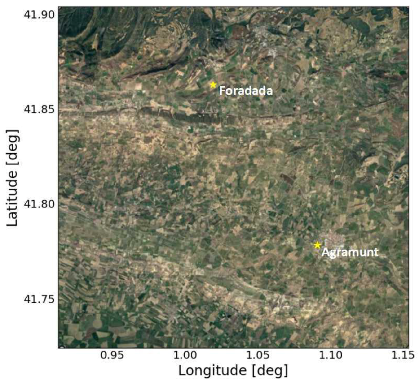
An old irrigated district located in this region has an open channel (built in 1862) transporting water towards the agricultural fields, thus allowing the vegetation to flourish in this specific area. Although the land surrounding the irrigated area is much drier, and a new irrigation network is being developed to augment the coverage of the old irrigation system, its influence is not yet visible on satellite imagery. The locations of two demonstration fields (inside the new irrigation area, at Foradada and Agramunt) are shown in Figure 1.
2.2. Database
2.2.1. Ground Measurements
In-situ soil moisture measurements were acquired continuously (5 min sampling frequency) over a period of several months, in two demonstration fields belonging to the new irrigation district: Foradada and Agramunt (Figure 1). Each measurement point was analyzed at different depths. The precipitation data comes from the nearest meteorological station to the demonstration field. For Foradada field, the Baldomar station, which is about 6 km away, is taken, while for Agramunt field, the Tornabous station, which is about 11 km, is considered. Table 1 lists the measured soil moisture and texture characteristics of the two test fields.
2.2.2. Satellite Data
(1) Sentinel-1 data
The Sentinel-1 satellites are equipped with C-band Synthetic Aperture Radar (SAR) instruments, providing data in dual or single polarizations. Sentinel-1 provides data with a spatial resolution of 10 m and a temporal resolution of 12 days, in both VV and VH polarizations. In the present study, signals recorded in the VV polarization were used to compute the soil moisture estimations. Only one ground track (110) was considered, for which the incidence angle was approximately 40.3°. Previous studies have shown that VH data has only a limited potential for the estimation of soil moisture, in particular as a consequence of its high sensitivity to volume scattering, which depends strongly on the geometrical alignment and characteristics of the vegetation [75,76,77]. The Sentinel-1 satellite database corresponds to the period from July 2015 to November 2016 (Table 2). All of the Sentinel-1 data was pre-processed using the Sentinel-1 Toolbox, in three steps:
- -
- Thermal noise removal
- -
- Radiometric calibration
- -
- Terrain correction using SRTM DEM at 30 m.
The last step is needed to average the data over 100 m pixels or cells. As discussed above, the methodologies proposed in this study were developed on the basis of this spatial resolution, which also has the advantage of eliminating speckle effects in the radar data.
(2) Sentinel-2 data
The Sentinel-2A satellite was launched in June 2015, and was followed by Sentinel-2B in March 2017. It is a wide-swath, high-resolution, multi-spectral imaging mission, and is designed to provide full and systematic coverage of the Earth’s land surfaces [78]. The Sentinel-2 database corresponds to the period from July 2015 to November 2016 (Table 3). The Sentinel-2 data corresponds to images recorded in 13 spectral bands, with a spatial resolution of 10 m. In the present study, band 4 (Red) and band 8 (NIR) are used to calculate the NDVI:
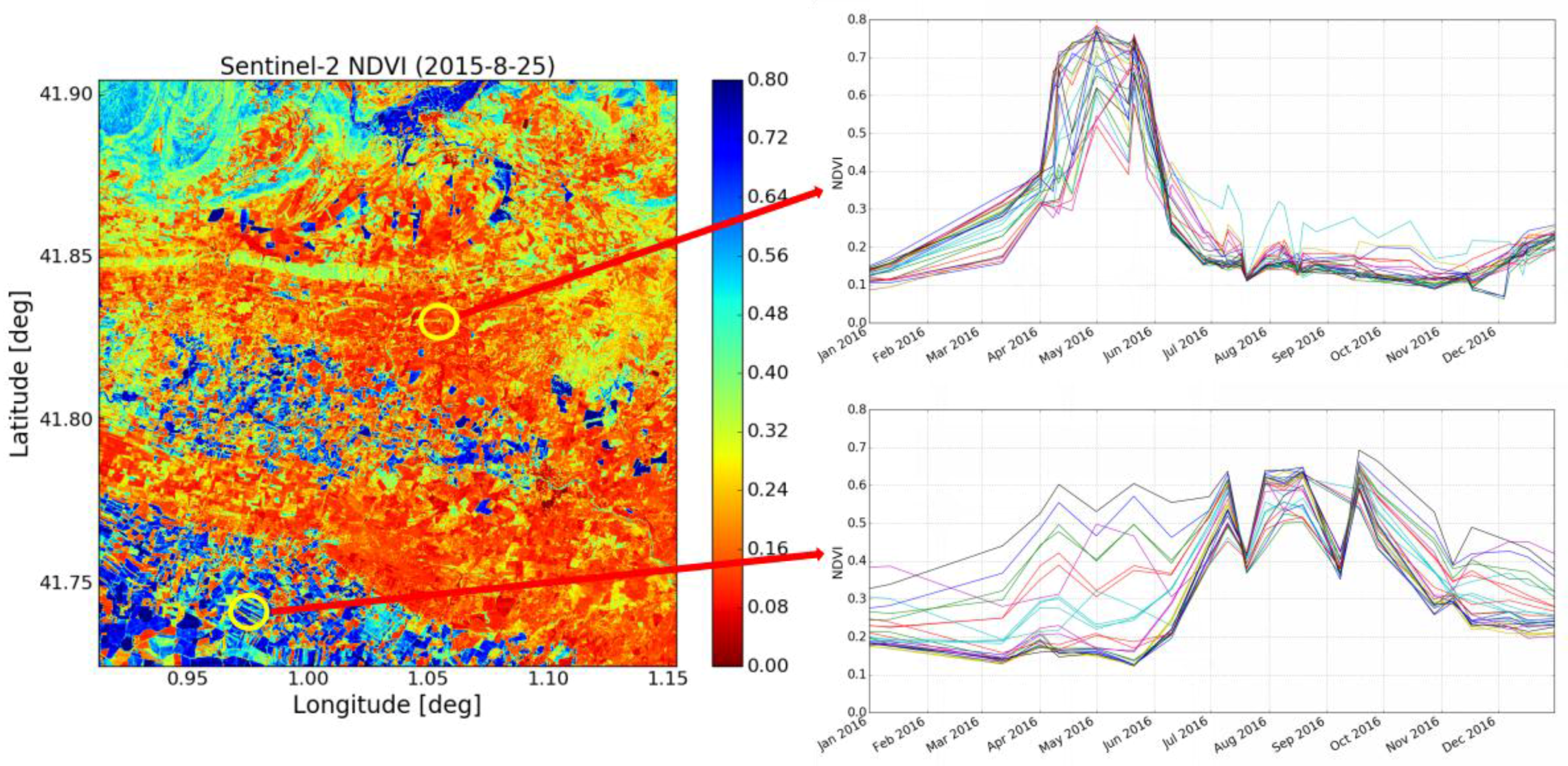
Band “QA60”, which is a bit-mask band containing cloud mask information, is applied in order to remove areas covered by cloud. Figure 2 is a NDVI map of our study area, computed from Sentinel-2 data recorded on 25 August 2015, and characterized by a dynamic range between 0.1 and 0.8. The temporal variations in NDVI during 2016 are shown for two different locations:
- -
- The first of these corresponds to dry (non-irrigated) land, revealing an NDVI cycle that occurs between April and July, with a low NDVI for the remaining periods of the year. This trend is confirmed for all of the pixels observed at this location.
- -
- The second site corresponds to an irrigated area, which is characterized by a broad range of spatial and temporal variations in NDVI.
In order to develop suitable soil moisture algorithms, a mask is used to remove high density vegetation areas with an NDVI > 0.8, corresponding to forests that are not encountered in the agricultural pixels, and low density vegetation areas with an NDVI < 0.1, corresponding to water surfaces.
3. Proposed Methodologies
3.1. Method 1 Description
The first method involves retrieval of soil moisture using the radar signal CD technique. This approach to soil water content estimations has already been applied to data recorded by the ERS Scatterometer over West Africa [15]. In the present study, this method was adapted to the characteristics of the Sentinel-1 observations, and the inversion algorithm was optimized to take advantage of the high repeat rate of this data. The radar signals backscattered by the surface can be modeled as the sum of the radar signals scattered by the bare soil and attenuated by vegetation effects, and the signals scattered by the vegetation cover. These two contributions can be expressed as:
where is the two-way vegetation canopy transmissivity, is the incidence angle and is the optical thickness parameter that depends on the type of geometrical structure and vegetation water content of the canopy [79].
Temporal variations in soil moisture can be directly related to the dynamics of the radar signal. When radar signals are considered for the same 100 × 100 m cell, and for approximately the same NDVI index, the roughness effect can be considerably reduced by computing the difference between two radar signals recorded at two dates.
For a given NDVI (retrieved from S2 data), by taking all of the corresponding radar data into account, the minimum value of σ0, corresponding to the driest signal, can be determined for each cell. The radar signal difference for a given cell (i,j), between one radar signal at date d and the driest signal, can be written as follows:
where is the backscattered signal from cell (i,j) at date d, with the corresponding NDVI computed from the (S2) optical images; is the lowest backscattered signal, corresponding to the driest conditions, and computed using the S1 time-series using the same NDVI as for the data recorded on date d (), and is a function of the NDVI and soil moisture Mv in cell (i,j).
As our radar database covers a period of only 1.5 years (due to the later launch date of the Sentinel-2 satellite, i.e., June 2015), it was not possible to retrieve this relationship for each value of NDVI. We thus consider NDVI classes for the computation of , using intervals of 0.1 (0.1–0.2, 0.2–0.3, 0.3–0.4, etc.). In the present case, the NDVI over the studied agricultural site ranges between a minimum of 0.1 and a maximum of 0.8.
Various experimental studies have shown that a linear relationship exists between radar signal differences and changes in soil moisture [19,80], in the case of bare soils and vegetation-covered surfaces. For a given NDVI, the radar signal difference, , can thus be written as:
where ∆ is the change in soil moisture between the date d and the date when the soil was at its driest. The parameter α depends on the NDVI.
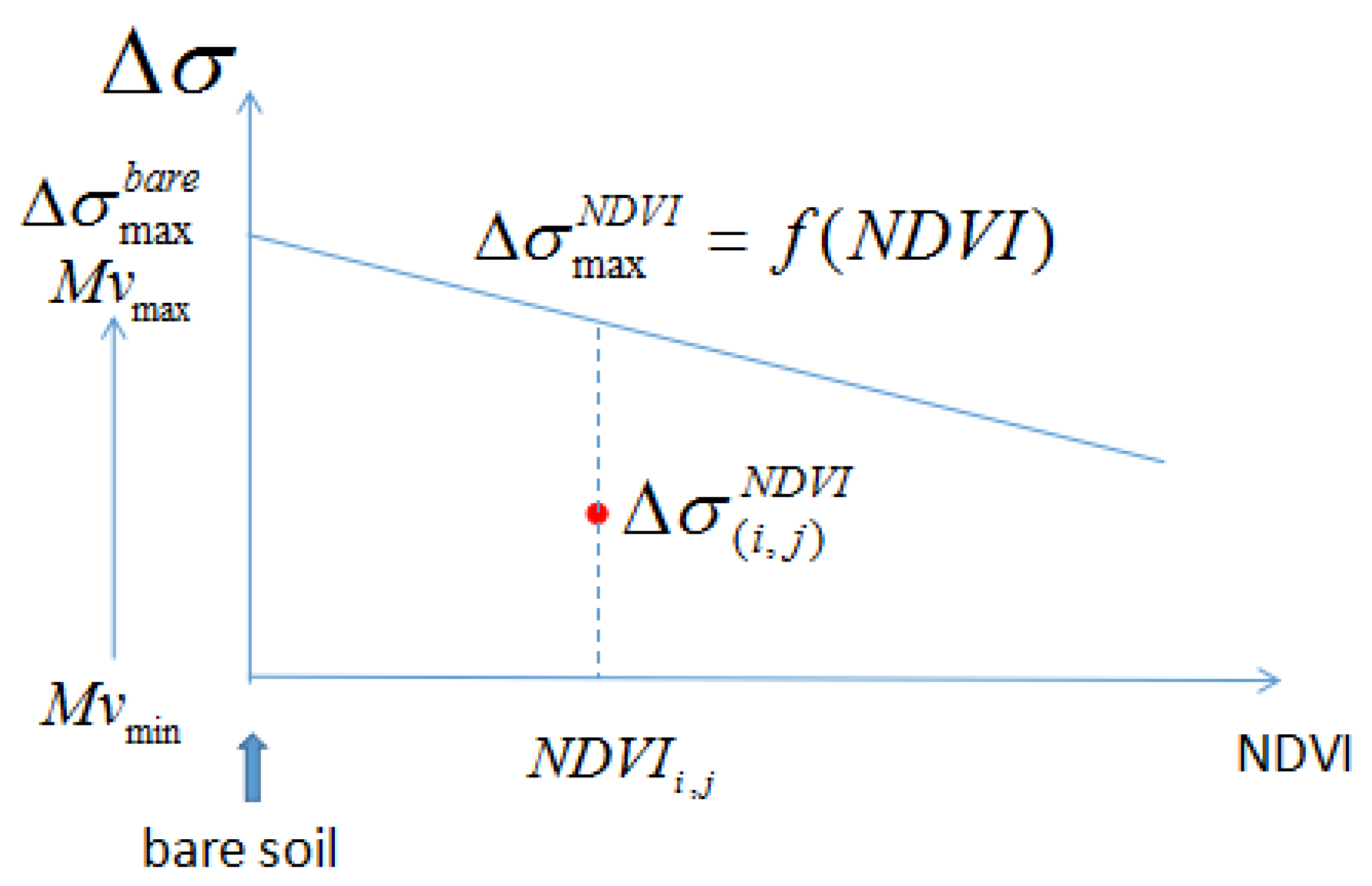
When the NDVI increases, the moisture sensitivity of the signal can be expected to decrease [22,81], as shown in Figure 3. This means that the difference between surface backscattering at a given date d, and that observed on the driest date, decreases as a function of NDVI.
The strongest variation in moisture, , corresponding to the difference between the driest value (Mvmin) and the wettest conditions (Mvmax), can be written as:
Under the conditions for which is defined, the maximum variation in backscattered signal (for a fixed value of NDVI), can be written as:
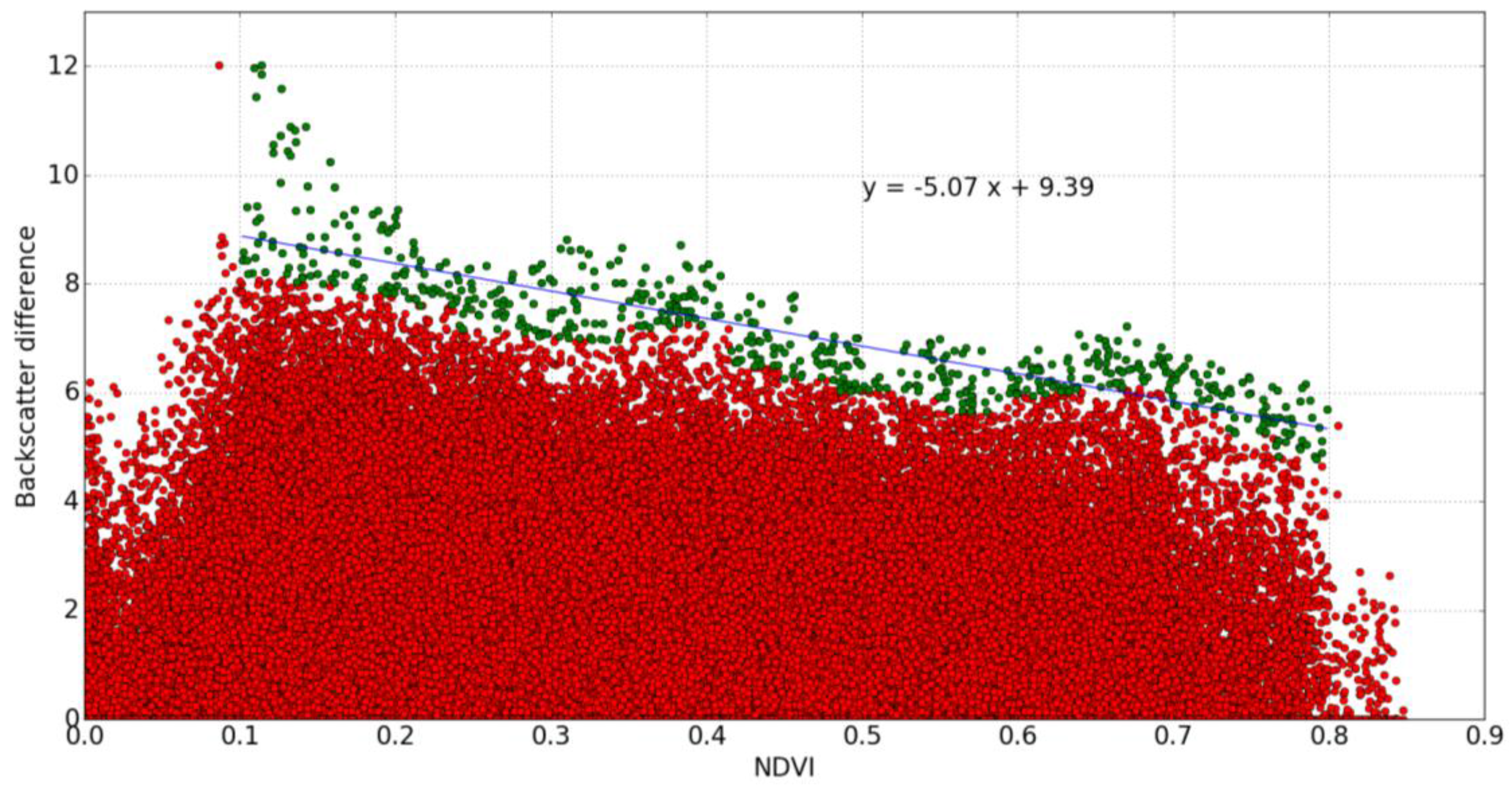
The predicted values of backscattered signal difference, corresponding to S1 data, are shown as a function of NDVI in Figure 4. The backscattering difference calculations were carried out for all cells and all S1 acquisition dates (over a period of approximately two years).
is modeled as [15]:
When NDVI = 0, , which corresponds to the maximum value of backscattering difference under the driest, bare-soil conditions.
In order to minimize the influence of noise when estimating , for each selected value of NDVI, we excluded the upper 1% of the corresponding values of radar signal difference, as well as all data points having a radar signal lower than −15 dB, since these are known to correspond to water [46,82] (Figure 4).
The soil moisture for each pixel can thus be retrieved using the following function:
SMOS low-resolution moisture products (SMOS Level 3 daily product), corresponding to the two-year period of S1 acquisitions, were used to estimate and , since the ground measurements were recorded for a limited period of time. The mean S1 radar signal is estimated over a SMOS pixel (40 km × 40 km). Figure 5 plots the relationship between this mean radar signal and the SMOS moisture values, for dates that are common to both SMOS and S1 acquisitions. An approximately linear relationship is found between the values of volumetric soil moisture and the backscattered radar signal, up to Mvmax ≈ 0.32 m3/m3, following which it saturates with a constant radar signal strength of approximately −9.5 dB. This result confirms the findings of several scientific studies, which have revealed radar signal saturation for soil moisture levels in the range (0.3–0.35 m3/m3) [21,81]. From this result, when using method 1 we consider = 0.32 m3/m3. As shown shown in Figure 5, the value of is taken to be ≈ 0.05 m3/m3.
3.2. Method 2 Description
A second change detection approach is proposed in this paper. This is based on the difference in backscattered signals observed on two consecutive days of Sentinel-1 data (12 days). Under these conditions, the temporal change in vegetation cover is generally very small such that, for a nearly constant value of roughness and constant vegetation conditions, the difference between the backscattered signals depends mainly on the change in soil moisture [24].
When the value of the NDVI increases, the radar signals’ sensitivity to temporal variations in moisture decreases. This means that the absolute value of the S1 radar signal difference decreases over two consecutive days, provided that the NDVI remains approximately stable on these two dates. In the present case, the latter parameter is taken to be the average of the NDVI values observed for the two consecutive dates. Figure 6 shows this change (either negative or positive) in radar signal behavior for successive S1 acquisitions, as a function of NDVI. is the maximum change in radar signal, corresponding to the maximum value of soil moisture change , for a given value of NDVI. This can be modeled by the empirical function g:
Figure 7 shows the difference in radar signal between two consecutive dates, as a function of NDVI, for all cells (i,j) and all NDVI levels at the Urgell site. The radar signal difference (negative or positive) between two adjacent days decreases in absolute value, when the NDVI increases. The negative or positive radar signal differences, resulting from respectively increasing or decreasing values of soil moisture, can be seen to follow a symmetrical, linear pattern.
In the case of the maximum value of soil moisture change , the function g can be written as:
where is the maximum radar signal difference between two consecutive measurements over bare soil, associated with the highest value of moisture change.
When the NDVI is equal to zero, is equal to , where b is the slope of the empirical function g. This describes the decrease in radar signal sensitivity to soil moisture. We observe an approximately symmetrical result in the computed values for the upper and lower limits. This is due to the fact that for a given value of mean soil moisture, a very similar behavior results from either a decrease or an increase in soil moisture, as these are linearly related to the radar signal.
In order to minimize the influence of noise arising from rare events, when estimating the function , for each selected value of NDVI we exclude the upper 1% of the corresponding values.
For a given NDVI, the backscatter difference , with t1 and t2 being adjacent S1 acquisition dates, is assumed to be linearly correlated with the soil moisture difference. The soil moisture difference for each cell (i,j), between successive acquisition dates t1 and t2, can be retrieved using the following function:
where H is equal to:
From the ground measurement statistics, the maximum soil moisture difference between two adjacent dates of Sentinel-1 data, , is assumed to be equal to 0.15 m3/m3.
From a starting date t1, which in the present case is a date corresponding to a ground measurement, an iterative calculation is used to determine the soil moisture for the following dates t1, t2, t3, …:
4. Results and Discussion
4.1. Results
Using ground measurements recorded in the Foradada field from May to August 2015, and from February to October 2016, and in the Agramunt field from May to October 2015, and from July to November 2016, the values of retrieved soil moisture were validated with Sentinel-1 data, using the two approaches described in the previous section. We compare the satellite estimations with surface moisture measurements obtained at a depth of 3 cm in the Foradada field, and at a depth of 5 cm in the Agramunt field.
4.1.1. Method 1 Validation with Ground Measurements
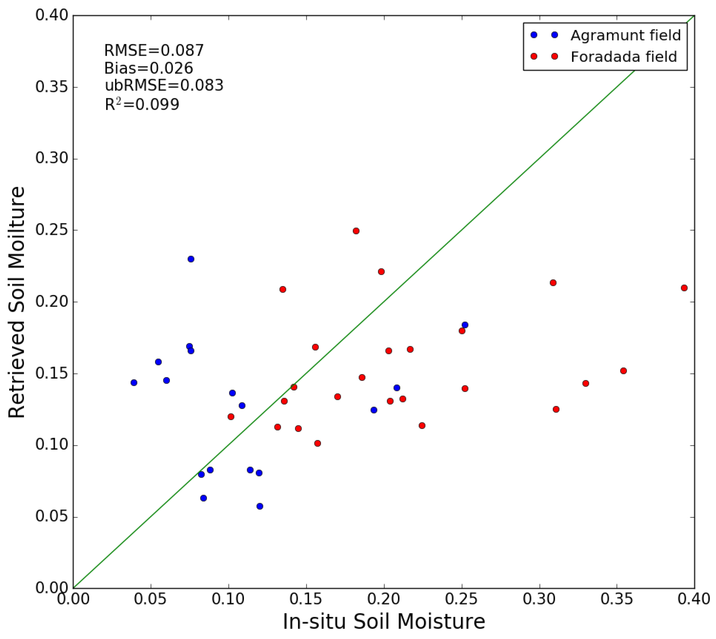
Figure 8 compares the ground measurements with the values of soil moisture modeled using method 1. The Root Mean Square (RMS) error in volumetric soil moisture is 0.087 m3/m3, with a bias of approximately 0.026 m3/m3. For Agramunt field, the RMSE is 0.074 m3/m3, with a bias of −0.019 m3/m3 and for Foradada field, the RMSE is 0.095 m3/m3, with a bias of 0.057 m3/m3. The RMSE can be estimated more reliably by defining an unbiased RMSE [83]:
where E[·] is the expectation operator. The unbiased RMSE corresponding to the first method is 0.083 m3/m3, which is equal to 0.071 m3/m3 for Agramunt field, and to 0.076 m3/m3 for Foradada field.
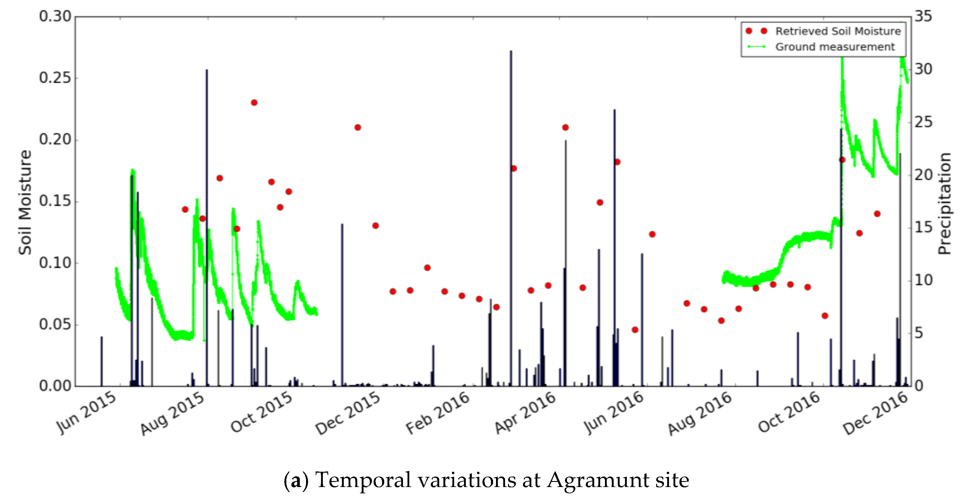
It can be seen that the errors are particularly high in the case of high moisture levels. This is due to possible variations in saturation moisture levels, and/or to spatial variations in soil roughness at the studied site. The statistical analysis should be improved by using a larger number of data acquisitions from the S1 time series. This can be expected to improve calibration of the function f. Figure 9 compares the soil moisture estimations with the ground measurements, as a function of time. The soil moisture levels retrieved from the satellite data are well correlated with precipitation events: a strong increase in soil moisture is observed, following each significant rainfall event.
4.1.2. Method 2 Validation with Ground Measurements
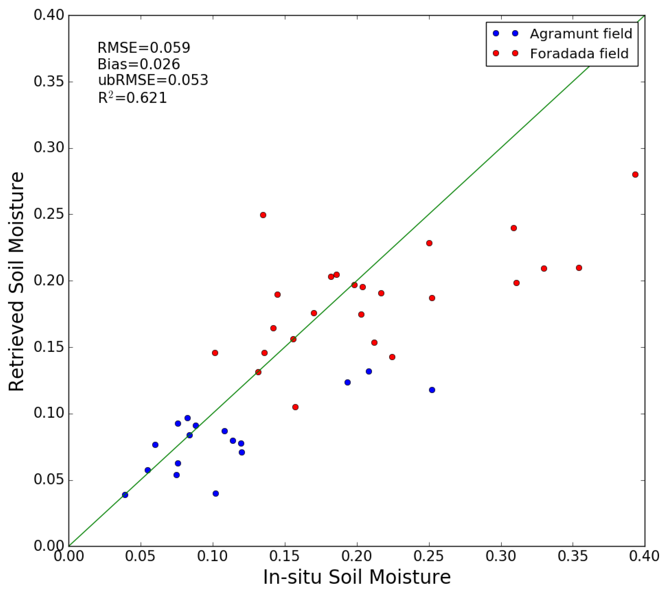
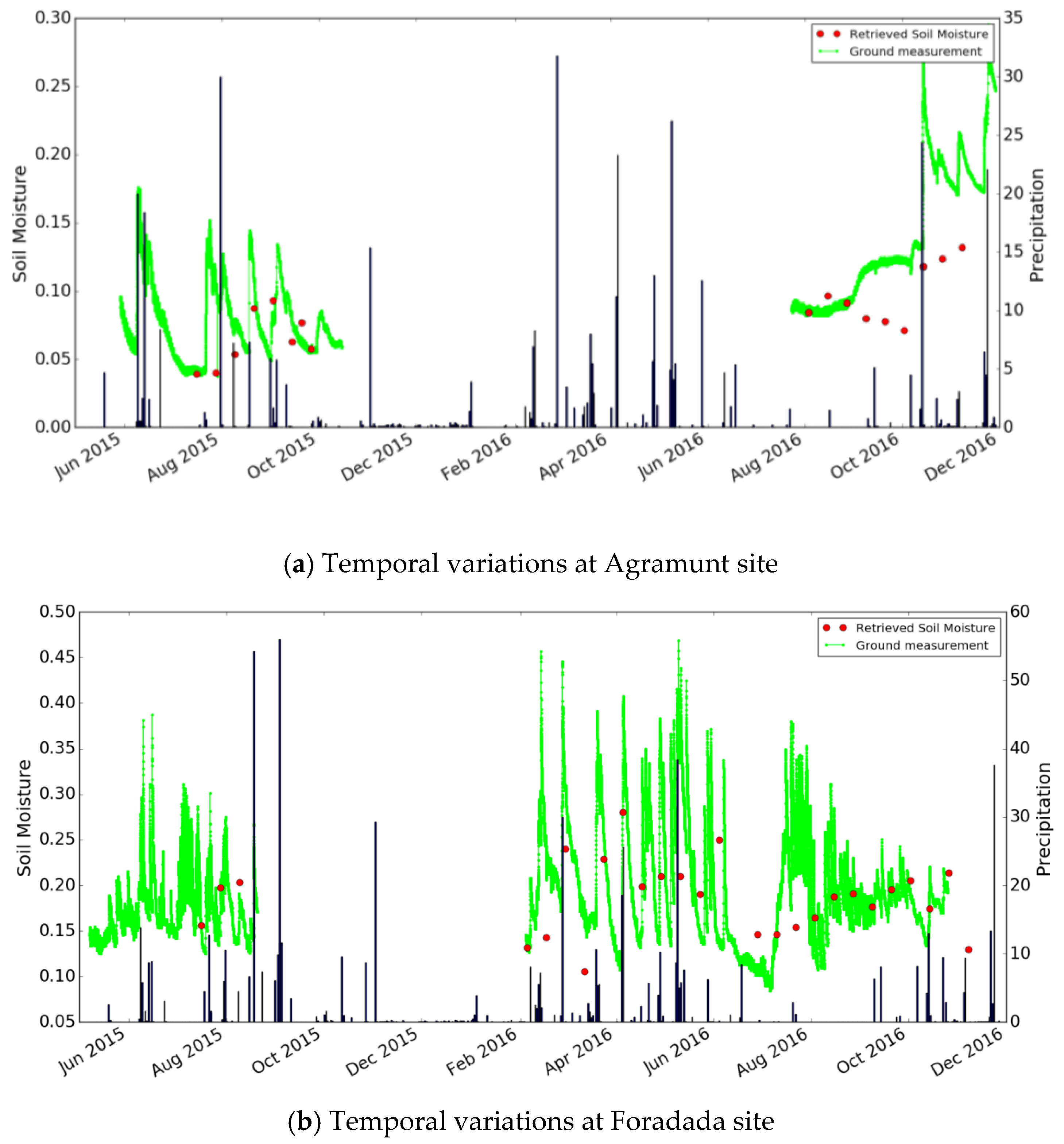
Figure 10 compares the ground measurements with the estimated values of soil moisture obtained with method 2. From this regression, the RMSE in volumetric soil moisture is 0.059 m3/m3, and the unbiased RMSE is 0.053 m3/m3. The RMSE is respectively equal to 0.048 m3/m3 and 0.066 m3/m3 for Agramunt and Foradada field, with a bias of 0.028 m3/m3 and 0.026 m3/m3 separately. The unbiased RMSE is 0.04 m3/m3 for Agramunt field and 0.06 m3/m3 for Foradada field. Figure 11 compares the moisture estimations with ground measurements, as a function of time. The soil moisture values retrieved from satellite data are also well correlated with the observed precipitation events, with the soil moisture increasing after each significant rainfall event. As both method1 and method 2 have a relatively high RMSE, the small number of ground measurements and the relatively small size of the radar signal database could explain this high error.
4.2. Discussion
The soil moisture at two study sites has been computed and mapped, using Equations (5)–(11) and data produced by Sentinel-1 radar observations. Figure 12 provides two illustrations of moisture mapping, using methods 1 and 2, for two cases: a very dry day (21 August 2015) and a wet day (2 September 2015). All cells with NDVI < 0.1 or NDVI > 0.8, which are associated with water bodies and forests respectively, are masked out. A high similarity is observed between the products obtained with these two methods. We retrieve nearly the same spatial variations in moisture on the two analyzed dates. The first dry case clearly reveals the irrigated fields inside dry area. The second wet case shows high values of soil moisture over most of the observed area.
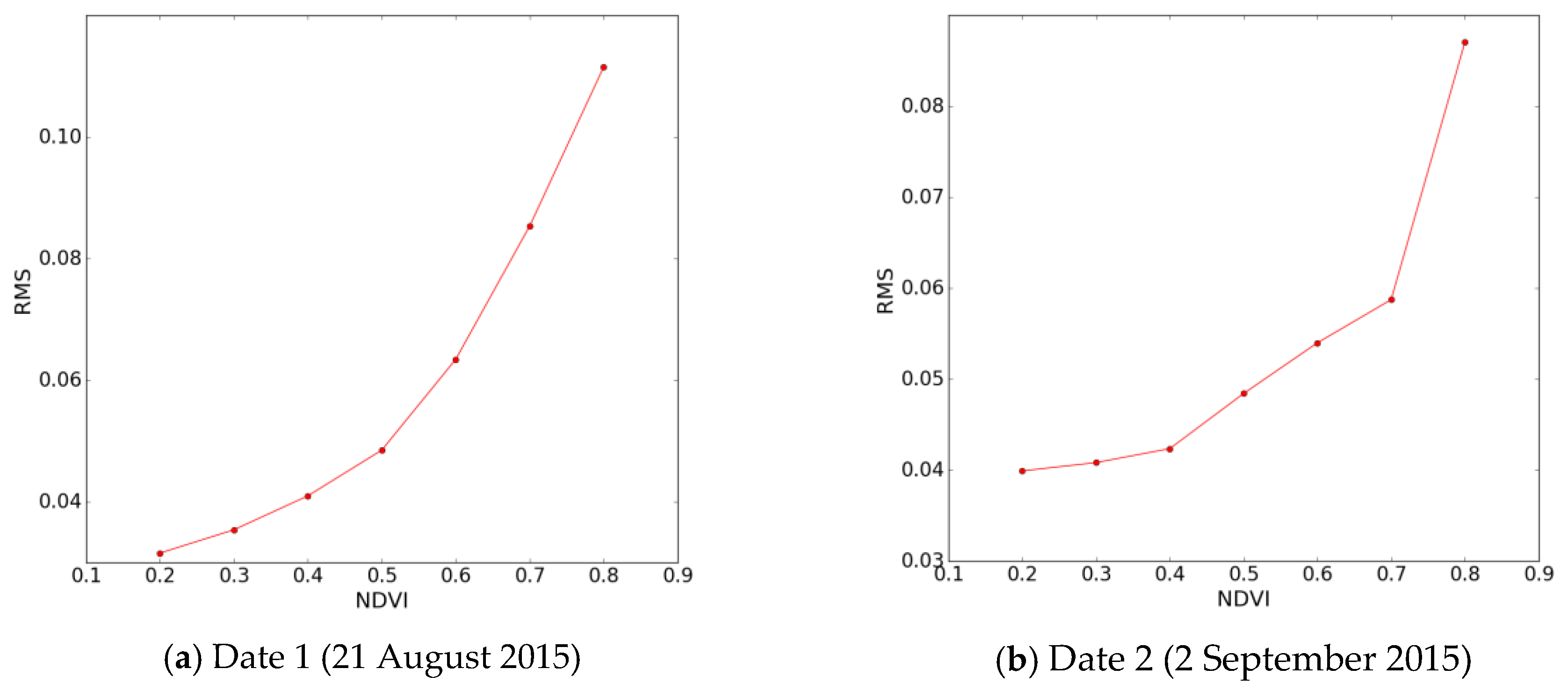
Figure 13 shows the difference between method 1 and method 2 for date 21 August 2015 and date 2 September 2015. A limited difference is illustrated for the two dates between the two methods. The highest differences correspond to high vegetation density covers. Figure 14 plots the variation in RMSE between methods 1 and 2, as a function of NDVI. This is estimated with a sliding NDVI window, with an NDVI width = 0.2, for NDVI values lying in the range between 0.1 and 0.8. The RMSE can be seen to increase with NDVI. In practice, a high vegetation density can significantly attenuate the signals, thus leading to correspondingly higher errors in soil moisture estimation. Areas with higher vegetation cover are with higher uncertainties. Rapid vegetation change and soil properties such as surface roughness will contribute to uncertainties as well. As change detection approaches, these two methods are very applied operationally since the ground measurements are not prerequisite and that they can be improved with the size of time series.
5. Conclusions
In this study, two inversion approaches are developed for the interpretation of high repeat frequency Sentinel-1 radar data in synergy with Sentinel-2 optical data. Change detection techniques in proposed methodologies, are validated with ground measurements carried out in two demonstration fields. The estimated (volumetric) RMS soil moisture errors are approximately 0.087 m3/m3 for method 1 and 0.059 m3/m3 for method 2. Both methods are found to predict soil moisture variations that are well correlated with rainfall events. Method 1 models the backscattering difference with the driest value, whereas method 2 is based on the difference between radar signals observed on two consecutive dates, meaning that the radar signals are influenced by much smaller changes in vegetation. Method 2 is found to be more robust than method 1, since it does not require searching for the minimum value in each pixel, which can introduce larger errors under extreme local conditions. The backscattered radar contributions produced by the vegetation are small in the case of method 2. However, as the retrieved value of soil moisture depends on the soil moisture determined at an earlier date with this method, the iterative process can lead to the accumulation of errors. Comparing to other types of inversion algorithms (e.g., NN or calibrated model inversion), both of these methods allow soil moisture to be estimated, with no need for calibrations based on ground measurements, and have led to the production of similar, 100 m resolution soil moisture maps of the study area. SMOS data is used for limiting the maximum soil moisture retrieved by satellite. However, the interest of SMOS (or SMAP or other low-resolution soil moisture sensor) is that it is available globally and needs no local maintenance, which makes our method applicable globally in contrast with methods that require in-situ data such as NN or calibrated model inversion.
These results demonstrate the potential of Sentinel-1 data for the retrieval of 100 m (or even better) resolution soil moisture. Both methods can be applied to any vegetation-covered area for which time-series of SAR and optical data have been recorded. In future, the statistical analysis should be improved by using a larger number of data acquisitions from the S1 time series.
In the present study, data derived from the VV polarization was analyzed, since it is more sensitive to soil conditions. However, Sentinel-1 provides data in both VV and VH polarization modes, and it is planned to include VH polarization analyses in future studies, since this operational mode is highly sensitive to the influence of vegetation, and can be used to discriminate between the effects of vegetation.
Acknowledgments
This study is part of the REC project partially funded by the European Commission Horizon 2020 Programme for Research and Innovation (H2020) in the context of the Marie Skłodowska-Curie Research and Innovation Staff Exchange (RISE) action under grant agreement No. 645642 and TOSCA/CNES ASCAS projects. The authors wish to thank the technical teams for their support and contributions to the successful ground campaigns.
Author Contributions
Q.G. and M.Z. conceived, designed and implemented the research. Q.G. performed the processing and drafted the manuscript. M.J.E. and N.B. provided suggestions and revised the manuscript.
Conflicts of Interest
The authors declare no conflict of interest.
References
- Aubert, D.; Loumagne, C.; Oudin, L. Sequential assimilation of soil moisture and streamflow data in a conceptual rainfall-runoff model. J. Hydrol. 2003, 280, 145–161. [Google Scholar] [CrossRef]
- Wagner, W.; Bloeschl, G.; Pamaloni, P.; Calvet, J. Operational readiness of microwave romote sensing of soil moisture for hydrologic applications. Nord. Hydrol. 2007, 38, 1–20. [Google Scholar] [CrossRef]
- Cook, B.I.; Bonan, G.B.; Levis, S. Soil moisture feedbacks to precipitation in Southern Africa. J. Clim. 2006, 19, 4198–4206. [Google Scholar] [CrossRef]
- Bezerra, B.G.; Santos, C.A.C.; Silva, B.B.; Perez-Marin, A.M.; Bezerra, M.V.C.; Berzerra, J.R.C.; Rao, T.V.R. Estimation of soil moisture in the root-zone from remote sensing data. Rev. Bras. Cienc. Solo 2013, 37, 596–603. [Google Scholar] [CrossRef]
- Pratola, C.; Barrett, B.; Gruber, A.; Dwyer, E. Quality Assessment of the CCI ECV Soil Moisture Product Using ENVISAT ASAR Wide Swath Data over Spain, Ireland and Finland. Remote Sens. 2015, 7, 15388–15423. [Google Scholar] [CrossRef]
- Barrett, B.; Petropoulos, G.P. Satellite Remote Sensing of Surface Soil Moisture. In Remote Sensing of Energy Fluxes and Soil Moisture Content; CRC Press: Boca Raton, FL, USA, 2013; pp. 85–120. ISBN 978-1-4665-0578-0. [Google Scholar]
- Petropoulos, G.P.; Ireland, G.; Barrett, B. Surface soil moisture retrievals from remote sensing: Current status, products and future trends. Phys. Chem. Earth 2015, 83, 36–56. [Google Scholar] [CrossRef]
- Zhuo, L.; Han, D. The relevance of soil moisture by remote sensing and hydrological modelling. Procedia Eng. 2016, 154, 1368–1375. [Google Scholar] [CrossRef]
- Alexandridis, T.K.; Cherif, I.; Bilas, G.; Almeida, W.G.; Hartanto, I.M.; van Andel, S.J.; Araujo, A. Spatial and Temporal Distribution of Soil Moisture at the Catchment Scale Using Remotely-Sensed Energy Fluxes. Water 2016, 8, 32. [Google Scholar] [CrossRef] [Green Version]
- Wagner, W.; Lemoine, G.; Rott, H. A method for estimating soil moisture from ERS Scatterometer and soil data. Remote Sens. Environ. 1999, 70, 191–207. [Google Scholar] [CrossRef]
- Al Bitar, A.; Kerr, Y.; Merlin, O.; Cabot, F.; Wigneron, J.P. Global drought index from SMOS soil moisture. In Proceedings of the IEEE International Geoscience and Remote Sensing Symposium (IGARSS 2013), Melbourne, Australia, 21–26 July 2013. [Google Scholar]
- Kerr, Y.; Waldteufel, P.; Richaume, P.; Wigneron, J.; Ferrazzoli, P.; Mahmoodi, A.; Al Bitar, A.; Cabot, F.; Gruhier, C.; Juglea, S.; et al. The SMOS soil moisture retrieval algorithm. IEEE Trans. Geosci. Remote Sens. 2012, 50, 1384–1403. [Google Scholar] [CrossRef]
- Mecklenburg, S.; Font, J.; Crapolicchio, R. ESA’s soil moisture and ocean salinity mission: Mission performance and operations. IEEE Trans. Geosci. Remote Sens. 2012, 50, 1354–1366. [Google Scholar] [CrossRef] [Green Version]
- Entekhabi, D.; Njoku, E.G.; O’Neill, P.E.; Kellogg, K.H.; Crow, W.T.; Edelstein, W.N.; Entin, J.K.; Goodman, S.D.; Jackson, T.J. The soil moisture active passive (SMAP) mission. Proc. IEEE 2010, 98, 704–716. [Google Scholar] [CrossRef]
- Zribi, M.; Andre, C.; Decharme, B. A method for soil moisture estimation in Western Africa based on the ERS scatterometer. IEEE Trans. Geosci. Remote Sens. 2008, 46, 438–448. [Google Scholar] [CrossRef]
- Gorrab, A.; Zribi, M.; Baghdadi, N.; Mougenot, B.; Chabaane, Z.L. Potential of X-band TerraSAR-X and COSMO-SkyMed SAR data for the assessment of physical soil parameters. Remote Sens. 2015, 7, 747–766. [Google Scholar] [CrossRef] [Green Version]
- Baghdadi, N.; Gaultier, S.; King, C. Retrieving surface roughness and soil moisture from synthetic aperture radar (SAR) data using neural networks. Can. J. Remote Sens. 2002, 28, 701–711. [Google Scholar] [CrossRef]
- Zribi, M.; Gorrab, A.; Baghdadi, N. A new soil roughness parameter for the modelling of radar backscattering over bare soil. Remote Sens. Environ. 2014, 152, 62–73. [Google Scholar] [CrossRef] [Green Version]
- Srivastava, H.S.; Patel, P.; Sharma, Y.; Navalgund, R.R. Large-area soil moisture estimation using multi-incidence-angle RADARSAT-1 SAR data. IEEE Trans. Geosci. Remote Sens. 2009, 47, 2528–2535. [Google Scholar] [CrossRef]
- Zribi, M.; Saux-Picart, S.; André, C.; Descroix, L.; Ottle, C.; Kallel, A. Soil moisture mapping based on ASAR/ENVISAT radar data over a Sahelian region. Int. J. Remote Sens. 2007, 28, 3547–3565. [Google Scholar] [CrossRef]
- Zribi, M.; Baghdadi, N.; Holah, N.; Fafin, O. New methodology for soil surface moisture estimation and its application to ENVISAT-ASAR multi-incidence data inversion. Remote Sens. Environ. 2005, 96, 485–496. [Google Scholar] [CrossRef]
- Zribi, M.; Dechambre, M. A new empirical model to retrieve soil moisture and roughness from C-band radar data. Remote Sens. Environ. 2003, 84, 42–52. [Google Scholar] [CrossRef]
- El Hajj, M.; Baghdadi, N.; Belaud, G.; Zribi, M.; Cheviron, B.; Courault, D.; Charron, F. Irrigated grassland monitoring using a time series of TerraSAR-X and COSMO-SkyMed X-band SAR data. Remote Sens. 2014, 6, 10002–10032. [Google Scholar] [CrossRef] [Green Version]
- Aubert, M.; Baghdadi, N.N.; Zribi, M.; Ose, K.; El Hajj, M.; Vaudour, E.; Gonzalez-Sosa, E. Toward an operational bare soil moisture mapping using TerraSAR-X data acquired over agricultural areas. IEEE J. Sel. Top. Appl. Earth Obs. Remote Sens. 2013, 6, 900–916. [Google Scholar] [CrossRef] [Green Version]
- Baghdadi, N.; Saba, E.; Aubert, M.; Zribi, M.; Baup, F. Evaluation of radar backscattering models IEM, Oh, and Dubois for SAR data in X-band over bare soils. IEEE Geosci. Remote Sens. Lett. 2011, 8, 1160–1164. [Google Scholar] [CrossRef]
- Baghdadi, N.; Cresson, R.; Pottier, E.; Aubert, M.; Zribi, M.; Jacome, A.; Benabdallah, S. A potential use for the C-band polarimetric SAR parameters to characterize the soil surface over bare agriculture fields. IEEE Trans. Geosci. Remote Sens. 2012, 50, 3844–3858. [Google Scholar] [CrossRef] [Green Version]
- Gorrab, A.; Zribi, M.; Baghdadi, N.; Mougenot, B.; Chabaane, Z.L. Retrieval of both Soil Moisture and Texture Using TarraSAR-X Images. Remote Sens. 2015, 7, 10098–10116. [Google Scholar] [CrossRef] [Green Version]
- Hegarat-Mascle, L.; Zribi, M.; Alem, F.; Weisse, A.; Loumagne, C. Soil moisture estimation from ERS/SAR data: Toward an operational methodology. IEEE Trans. Geosci. Remote Sens. 2002, 40, 2647–2658. [Google Scholar] [CrossRef]
- Srivastava, H.S.; Patel, P.; Manchanda, M.L.; Adiga, S. Use of multiincidence angle RADARSAT-1 SAR data to incorporate the effect of surface roughness in soil moisture estimation. IEEE Trans. Geosci. Remote Sens. 2003, 41, 1638–1640. [Google Scholar] [CrossRef]
- Singh, D. A simplistic incidence angle approach to retrieve the soil moisture and surface roughness at X-band. IEEE Trans. Geosci. Remote Sens. 2005, 43, 2606–2611. [Google Scholar] [CrossRef]
- Anguela, T.P.; Zribi, M.; Baghdadi, N.; Loumagne, C. Analysis of local variation of soil surface parameters with TerraSAR-X radar data over bare agricultural fields. IEEE Trans. Geosci. Remote Sens. 2010, 48, 874–881. [Google Scholar] [CrossRef] [Green Version]
- Shi, J.; Wang, J.; Hsu, A.Y.; O’Neill, P.E.; Engman, E.T. Estimation of bare surface soil moisture and surface roughness parameter using L-band SAR image data. IEEE Trans. Geosci. Remote Sens. 1997, 35, 1254–1266. [Google Scholar] [CrossRef]
- Ponnurangam, G.G.; Rao, Y.S. Soil moisture mapping using ALOS PALSAR and ENVISAT ASAR data over India. In Proceedings of the 2011 3rd International Asia-Pacific Conference on Synthetic Aperture Radar (APSAR 2011), Seoul, Korea, 26–30 September 2011. [Google Scholar]
- Sonobe, R.; Tani, H.; Wang, X.; Fukuda, M. Estimation of soil moisture for bare soil fields using ALOS/PALSAR HH polarization data. Agric. Inf. Res. 2008, 17, 171–177. [Google Scholar] [CrossRef]
- Prevot, L.; Champion, I.; Guyot, G. Estimating surface soil moisture and leaf area index of a wheat canopy using a dual-frequency (C and X bands) scatterometer. Remote Sens. Environ. 1993, 46, 331–339. [Google Scholar] [CrossRef]
- De Roo, R.D.; Du, Y.; Ulaby, F.T.; Dobson, M.C. A semi-empirical backscattering model at L-band and C-band for a soybean canopy with soil moisture inversion. IEEE Trans. Geosci. Remote Sens. 2001, 39, 864–872. [Google Scholar] [CrossRef]
- Sikdar, M.; Cumming, I. A modified empirical model for soil moisture estimation in vegetated areas using SAR data. In Proceedings of the 2004 IEEE International Geoscience and Remote Sensing Symposium, Anchorage, AK, USA, 20–24 September 2004. [Google Scholar]
- Gherboudj, I.; Magagi, R.; Berg, A.A.; Toth, B. Soil moisture retrieval over agricultural fields from multi-polarized and multi-angular RADARSAT-2 SAR data. Remote Sens. Environ. 2011, 115, 33–43. [Google Scholar] [CrossRef]
- Wang, S.G.; Li, X.; Han, X.J.; Jin, R. Estimation of surface soil moisture and roughness from multi-angular ASAR imagery in the Watershed Allied Telemetry Experimental Research (WATER). Hydrol. Earth Syst. Sci. 2011, 15, 1415–1426. [Google Scholar] [CrossRef]
- Yu, F.; Zhao, Y. A new semi-empirical model for soil moisture content retrieval by ASAR and TM data in vegetation-covered areas. Sci. Chin. Earth Sci. 2011, 54, 1955–1964. [Google Scholar] [CrossRef]
- Zribi, M.; Chahbi, A.; Shabou, M.; Lili-Chabaane, Z.; Duchemin, B.; Baghdadi, N.; Amri, R.; Chehbouni, A. Soil surface moisture estimation over a semi-arid region using ENVISAT ASAR radar data for soil evaporation evaluation. Hydrol. Earth Syst. Sci. 2011, 15, 345–358. [Google Scholar] [CrossRef] [Green Version]
- Yang, G.; Shi, Y.; Zhao, C.; Wang, J. Estimation of soil moisture from multi-polarized SAR data over wheat coverage areas. In Proceedings of the 2012 First International Conference on Agro-Geoinformatics (Agro-Geoinformatics), Shanghai, China, 2–4 August 2012. [Google Scholar]
- Peng, J.; Loew, A.; Merlin, O.; Verhoest, N. A review of methods for downscaling remotely sensed soil moisture. Rev. Geophys. 2017, 55, 341–366. [Google Scholar] [CrossRef]
- Ulaby, F.T.; Moore, R.K.; Fung, A.K. Pysical mechanisms and empirical models for scattering and emission. Microw. Remote Sens. 1982, 2, 816–921. [Google Scholar]
- Sahebi, M.R.; Bonn, F.; Bénié, G.B. Neural networks for the inversion of soil surface parameters from synthetic aperture radar satellite data. Can. J. Civ. Eng. 2004, 31, 95–108. [Google Scholar] [CrossRef]
- Santi, E.; Paloscia, S.; Pettinato, S.; Notarnicola, C.; Pasolli, E.; Pistocchi, A. Comparison between SAR Soil Moisture Estimates and Hydrological Model Simulations over the Scrivia Test Site. Remote Sens. 2013, 5, 4961–4976. [Google Scholar] [CrossRef]
- Pham-Duc, B.; Prigent, C.; Aires, F. Surface Water Monitoring within Cambodia and the Vietnamese Mekong Delta over a Year, with Sentinel-1 SAR Observations. Water 2017, 9, 366. [Google Scholar] [CrossRef]
- Notarnicola, C.; Angiulli, M.; Posa, F. Soil moisture retrieval from remotely sensed data: Neural network approach versus bayesian method. IEEE Trans. Geosci. Remote Sens. 2008, 46, 547–557. [Google Scholar] [CrossRef]
- Pasquariello, G.; Satalino, G.; Mattia, F.; Casarano, D.; Posa, F.; Souyris, J.C.; Le Toan, T. On the retrieval of soil moisture from SAR data over bare soils. In Proceedings of the IEEE International Geoscience and Remote Sensing (IGARSS 1997), Singapore, 3–8 August 1997; Voulme 3, pp. 1272–1274. [Google Scholar]
- Baghdadi, N.; El Hajj, M.; Zribi, M.; Fayad, I. Coupling SAR C-band and optical data for soil moisture and leaf area index retrieval over irrigated grasslands. IEEE JSTARS 2016, 9, 1229–1243. [Google Scholar] [CrossRef]
- El Hajj, M.; Baghdadi, N.; Zribi, M.; Belaud, G.; Cheviron, B.; Courault, D.; Charron, F. Soil moisture retrieval over irrigated grassland using X-band SAR data. Remote Sens. Environ. 2016, 176, 202–218. [Google Scholar] [CrossRef]
- Baghdadi, N.; Cresson, R.; El Hajj, M.; Ludwig, R.; la Jeunesse, I. Estimation of soil parameters over bare agriculture areas from C-band polarimetric SAR data using neural networks. Hydrol. Earth Syst. Sci. 2012, 16, 1607–1621. [Google Scholar] [CrossRef] [Green Version]
- Santi, E.; Paloscia, S.; Pettinato, S.; Fontanelli, G. Application of artificial neural networks for the soil moisture retrieval from active and passive microwave spaceborne sensors. Int. J. Appl. Earth Obs. Geoinf. 2016, 48, 61–73. [Google Scholar] [CrossRef]
- Alexakis, D.D.; Mexis, F.K.; Vozinaki, A.K.; Daliakopoulos, I.N.; Tsanis, I.K. Soil Moisture Content Estimation Based on Sentinel-1 and Auxiliary Earth Observation Products. A Hydrological Approach. Sensors 2017, 17, 1455. [Google Scholar] [CrossRef] [PubMed]
- Attema, E.W.P.; Ulaby, F.T. Vegetation modelled as a water cloud. Radio Sci. 1978, 13, 357–364. [Google Scholar] [CrossRef]
- Chai, X.; Zhang, T.; Shao, Y.; Gong, H.; Liu, L.; Xie, K. Modeling and Mapping Soil Moisture of Plateau Pasture Using RADARSAT-2 Imagery. Remote Sens. 2015, 7, 1279–1299. [Google Scholar] [CrossRef]
- He, B.; Xing, M.; Bai, X. A Synergistic Methodology for Soil Moisture Estimation in an Alpine Prairie Using Radar and Optical Satellite Data. Remote Sens. 2014, 6, 10966–10985. [Google Scholar] [CrossRef]
- Kumar, K.; Suryanarayana Rao, H.P.; Arora, M.K. Study of water cloud model vegetation descriptors in estimating soil moisture in Solani catchment. Hydrol. Process. 2015, 29, 2137–2148. [Google Scholar] [CrossRef]
- Bai, X.; He, B.; Li, X.; Zeng, J.; Wang, X.; Wang, Z.; Zeng, Y.; Su, Z. First Assessment of Sentinel-1A Data for Surface Soil Moisture Estimations Using a Coupled Water Cloud Model and Advanced Integral Equation Model over the Tibetan Plateau. Remote Sens. 2017, 9, 714. [Google Scholar] [CrossRef]
- Thoma, D.P.; Moran, M.S.; Bryant, R.; Rahman, M.; Holifield-Collins, C.D.; Skirvin, S.; Sano, E.E.; Slocum, K. Comparison of four models to determine surface soil moisture from C-band radar imagery in a sparsely vegetated semiarid landscape. Water Resour. Res. 2006, 42, 1–12. [Google Scholar] [CrossRef]
- Thoma, D.; Moran, M.; Bryant, R.; Collins, C.H.; Rahman, M.; Skirvin, S. Comparison of two methods for extracting surface soil moisture from C-band radar imagery. In Proceedings of the IEEE International Geoscience and Remote Sensing Symposium (IGARSS 2004), Anchorage, AK, USA, 20–24 September 2004; pp. 827–830. [Google Scholar]
- Rignot, E.J.M.; van Zyl, J.J. Change detection techniques for ERS-1 SAR data. IEEE Trans. Geosci. Remote Sens. 1993, 31, 896–906. [Google Scholar] [CrossRef]
- Villasensor, J.D.; Fatland, D.R.; Hinzman, L.D. Change detection on Alaska’s North Slope using repeat-pass ERS-1 SAR images. IEEE Trans. Geosci. Remote Sens. 1993, 31, 227–236. [Google Scholar] [CrossRef]
- Shoshany, M.; Svoray, T.; Curran, P.J.; Foody, G.M.; Perevolotsky, A. The relationship between ERS-2 SAR backscatter and soil moisture: Generalization from a humid to semi-arid transect. Int. J. Remote Sens. 2000, 21, 2337–2343. [Google Scholar] [CrossRef]
- Thoma, D.P.; Moran, M.S.; Bryant, R.; Rahman, M.M.; Collins, C.D.H.; Keefer, T.O.; Noriega, R.; Osman, I.; Skrivin, S.M.; Tischler, M.A.; et al. Appropriate scale of soil moisture retrieval from high resolution radar imagery for bare and minimally vegetated soils. Remote Sens. Environ. 2008, 112, 403–414. [Google Scholar] [CrossRef]
- Jacome, A.; Bernier, M.; Chokmani, K.; Gauthier, Y.; Poulin, J.; De Sève, D. Monitoring Volumetric Surface Soil Moisture Content at the La Grande Basin Boreal Wetland by Radar Multi Polarization Data. Remote Sens. 2013, 5, 4919–4941. [Google Scholar] [CrossRef]
- Baghdadi, N.; Camus, P.; Beaugendre, N.; Malam Issa, O.; Zribi, M.; Desprats, J.F.; Rajot, J.L.; Abdallah, C.; Sannier, C. Estimating surface soil moisture from TerraSAR-X data over two small catchments in the sahelian part of western Niger. Remote Sens. 2011, 3, 1266–1283. [Google Scholar] [CrossRef] [Green Version]
- Zribi, M.; Kotti, F.; Amri, R.; Wagner, W.; Shabou, M.; LiliChabaane, Z.; Baghdadi, N. Soil moisture mapping in a semiarid region, based on ASAR/wide swath satellite data. Water Resour. Res. 2014, 50, 823–835. [Google Scholar] [CrossRef]
- Wagner, W.; Pathe, C.; Doubkova, M.; Sabel, D.; Bartsch, A.; Hasenauer, S.; Bloeschl, G.; Scipal, K.; Martinez-Fernandez, J.; Loew, A. Temporal stability of soil moisture and radar backscatter observed by the Advanced Synthetic Aperture Radar (ASAR). Sensors 2008, 8, 1174–1197. [Google Scholar] [CrossRef] [PubMed]
- Pulvirenti, L.; Ticconi, F.; Pierdicca, N. Neural Network Emulation of the Integral Equation Model with Multiple Scattering. Sensors 2009, 9, 8109–8125. [Google Scholar] [CrossRef] [PubMed]
- Fung, A.K.; Li, Z.; Chen, K.S. Backscattering from a randomly rough dielectric surface. IEEE Trans. Geosci. Remote Sens. 1992, 30, 356–369. [Google Scholar] [CrossRef]
- Gharechelou, S.; Tateishi, R.; Sri Sumantyo, J.T. Comparison of Simulated Backscattering Signal and ALOS PALSAR Backscattering over Arid Environment Using Experimental Measurement. Adv. Remote Sens. 2015, 4, 224–233. [Google Scholar] [CrossRef]
- Barrett, B.W.; Dwyer, E.; Whelan, P. Soil Moisture Retrieval from Active Spaceborne Microwave Observations: An Evaluation of Current Techniques. Remote Sens. 2009, 1, 210–242. [Google Scholar] [CrossRef]
- Escorihuela, M.J.; Quintana-Segui, P. Comparison of remote sensing and simulated soil moisture datasets in mediterranean landscapes. Remote Sens. Environ. 2016, 180, 99–114. [Google Scholar] [CrossRef]
- Karjalainen, M.; Kaartinen, H.; Hyyppä, J.; Laurila, H.; Kuittinen, R. The Use of ENVISAT Alternating Ploarization SAR Images in Agricultureal Monitoring in Compatison with RADARSAT-1 SAR Images. In Proceedings of the ISPRS Congress, Istanbul, Turkey, 12–23 July 2004. [Google Scholar]
- Patel, P.; Srivastava, H.S.; Panigrahy, S.; Parihar, J.S. Comparative evaluation of the sensitivity of multi-polarized multi-frequency SAR backscatter to plant density. Int. J. Remote Sens. 2006, 27, 293–305. [Google Scholar] [CrossRef]
- Chauhan, S.; Srivastava, H.S. Comparative evaluation of the sensitivity of multi-polarized SAR nd optical data for various land cover classed. Int. J. Remote Sens. 2016, 4, 01–14. [Google Scholar]
- Pesaresi, M.; Corbane, C.; Julea, A.; Florczyk, A.J.; Syrris, V.; Soille, P. Assessment of the Added-Value of Sentinel-2 for Detecting Built-up Areas. Remote Sens. 2016, 8, 299. [Google Scholar] [CrossRef] [Green Version]
- Gupta, V.K.; Sharma, N.; Jangid, R.A. Emission and scattering behaviour of bare and vegetative soil surfaces of different moist states by microwave remote sensing. Indian J. Radio Space Phys. 2013, 42, 42–51. [Google Scholar]
- Baghdadi, N.; Aubert, M.; Cerdan, O.; Franchistéguy, L.; Viel, C.; Martin, E.; Zribi, M.; Desprats, J.F. Operational Mapping of Soil Moisture Using Synthetic Aperture Radar Data: Application to the Touch Basin (France). Sensors 2007, 7, 2458–2483. [Google Scholar] [CrossRef]
- Baghdadi, N.; Cerdan, O.; Zribi, M.; Auzet, V.; Darboux, F.; El Hajj, M.; Kheir, R.B. Operational performance of current synthetic aperture radar sensors in mapping soil surface characteristics in agricultural environments: Application to hydrological and erosion modelling. Hydrol. Process. 2007, 22, 9–20. [Google Scholar] [CrossRef]
- Liu, C. Analysis of Sentinel-1 SAR Data for Mapping Standing Water in the Twente Region. Master’s Thesis, University of Twente, Twente, The Netherlands, February 2016. Available online: http://www.itc.nl/library/papers_2016/msc/wrem/cliu.pdf (accessed on 22 May 2017).
- Entekhabi, D.; Reichle, R.H.; Koster, R.D.; Crow, W.T. Performance Metrics for Soil Moisture Retrievals and Application Requirements. J. Hydrometeorol. 2010, 11, 832–840. [Google Scholar] [CrossRef]
Figure 1.
Study area in Urgell, Catalunya (20 km × 20 km) with ground measurements (yellow stars).

Figure 2.
Sentinel-2 NDVI map in the study area (left), NDVI time series for the dry land site (upper right), and NDVI time series for the site in the old irrigated area (lower right).
Figure 2.
Sentinel-2 NDVI map in the study area (left), NDVI time series for the dry land site (upper right), and NDVI time series for the site in the old irrigated area (lower right).

Figure 3.
Illustration of the relationship between NDVI and Mv used in method 1.

Figure 4.
Illustration of the processed radar signal differences (dB) for all dates, with the driest radar signals shown as a function of NDVI for all (100 m × 100 m) cells in the Urgell area. Each point corresponds to a single radar signal difference for a cell (i,j).
Figure 4.
Illustration of the processed radar signal differences (dB) for all dates, with the driest radar signals shown as a function of NDVI for all (100 m × 100 m) cells in the Urgell area. Each point corresponds to a single radar signal difference for a cell (i,j).

Figure 5.
Mean S1 radar signal as a function of the SMOS soil moisture computed over a single SMOS pixel (40 km × 40 km). The radar signal saturates beyond soil moisture levels of 0.32 m3/m3.
Figure 5.
Mean S1 radar signal as a function of the SMOS soil moisture computed over a single SMOS pixel (40 km × 40 km). The radar signal saturates beyond soil moisture levels of 0.32 m3/m3.
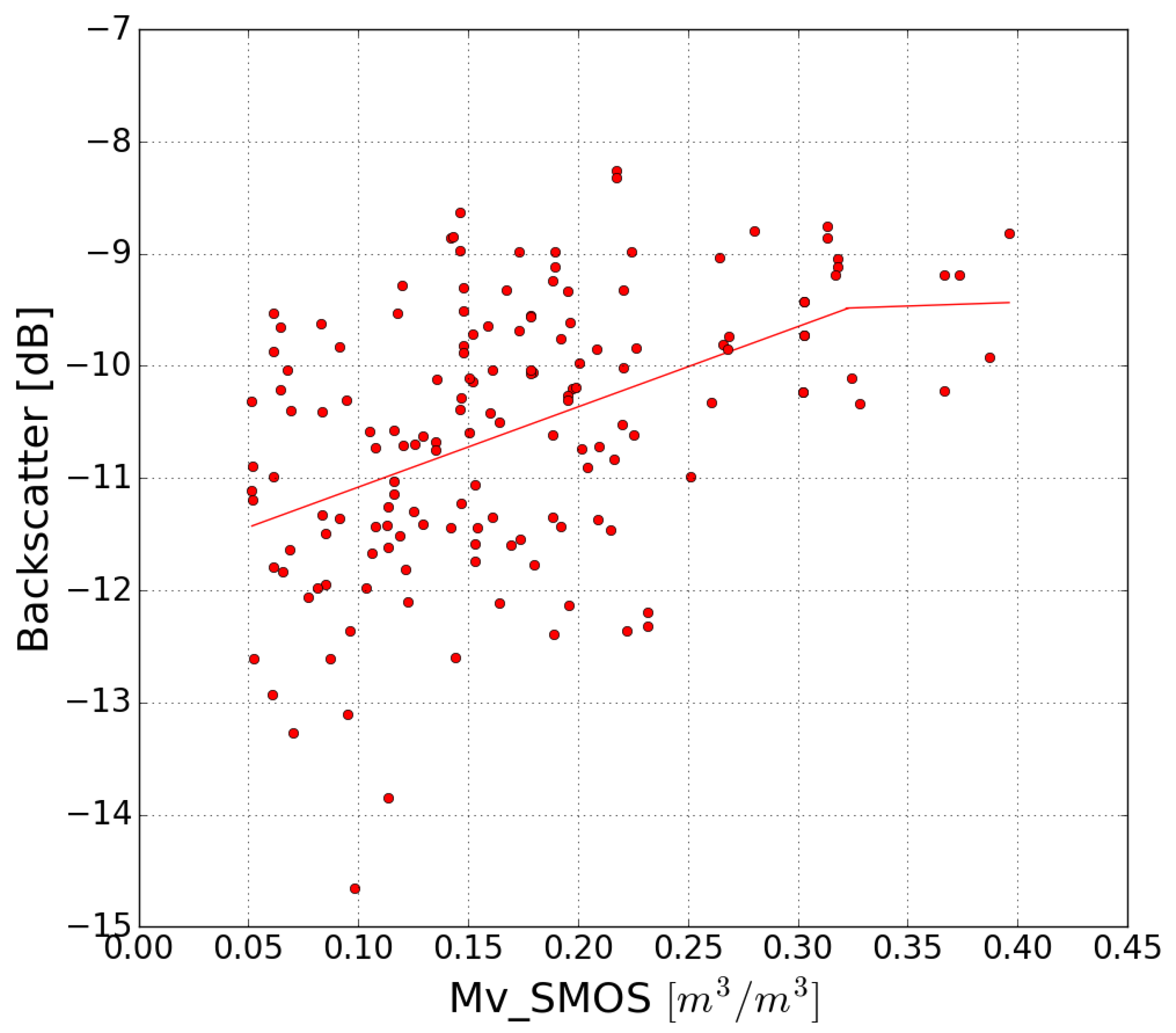
Figure 6.
Illustration of method 2.
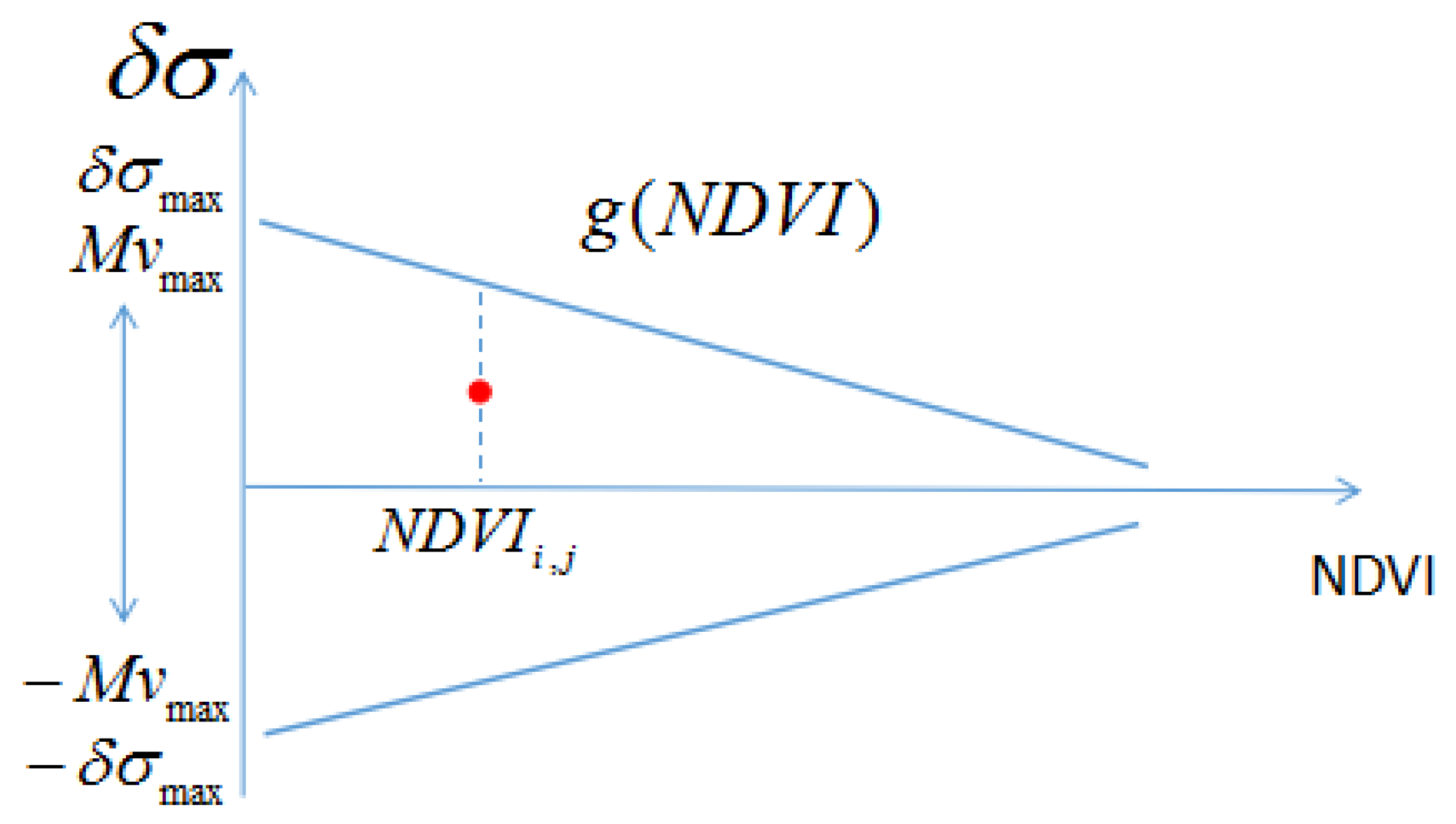
Figure 7.
Illustration of the radar signal difference (dB) computed for two consecutive dates, as a function of NDVI over the Urgell site. Each point corresponds to a single cell (i,j). For each value of NDVI, the green points indicate the upper decile of the corresponding differences in radar signal.
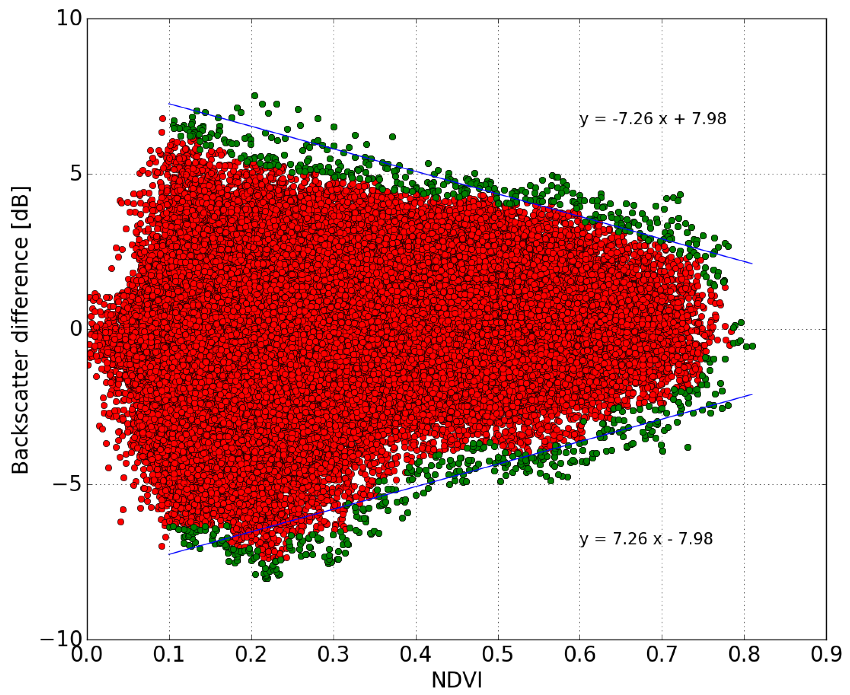
Figure 8.
Intercomparison between ground measurements and S1 moisture estimations based on method 1, for the case of two demonstration fields, at Agramunt and Foradada.
Figure 8.
Intercomparison between ground measurements and S1 moisture estimations based on method 1, for the case of two demonstration fields, at Agramunt and Foradada.

Figure 9.
Temporal variations in ground measurements and S1 estimations of soil moisture at the Agramunt site (a) and Foradada site (b).
Figure 9.
Temporal variations in ground measurements and S1 estimations of soil moisture at the Agramunt site (a) and Foradada site (b).

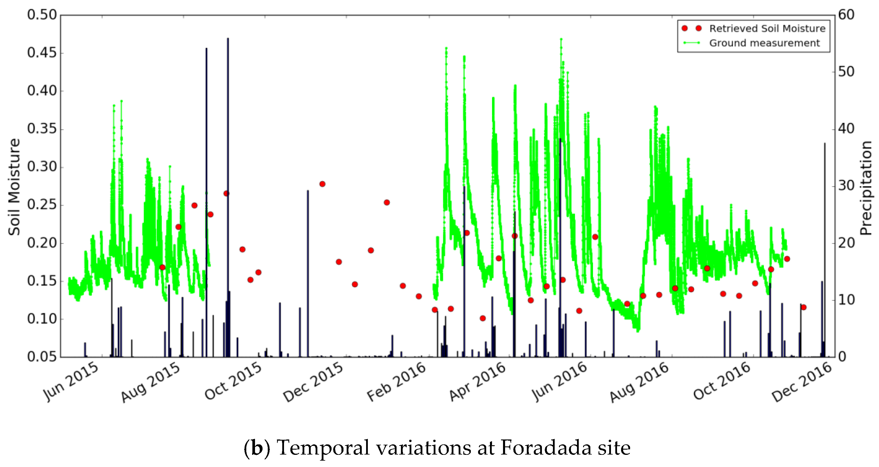
Figure 10.
Intercomparison between ground measurements in the two demonstration fields of Agramunt and Foradada and S1 moisture estimations based on method 2.
Figure 10.
Intercomparison between ground measurements in the two demonstration fields of Agramunt and Foradada and S1 moisture estimations based on method 2.

Figure 11.
Temporal variations in ground measurements and S1 estimations of soil moisture at the Agramunt site (a) and Foradada site (b), determined using method 2.
Figure 11.
Temporal variations in ground measurements and S1 estimations of soil moisture at the Agramunt site (a) and Foradada site (b), determined using method 2.

Figure 12.
Retrieved soil moisture maps obtained using methods 1 and 2.
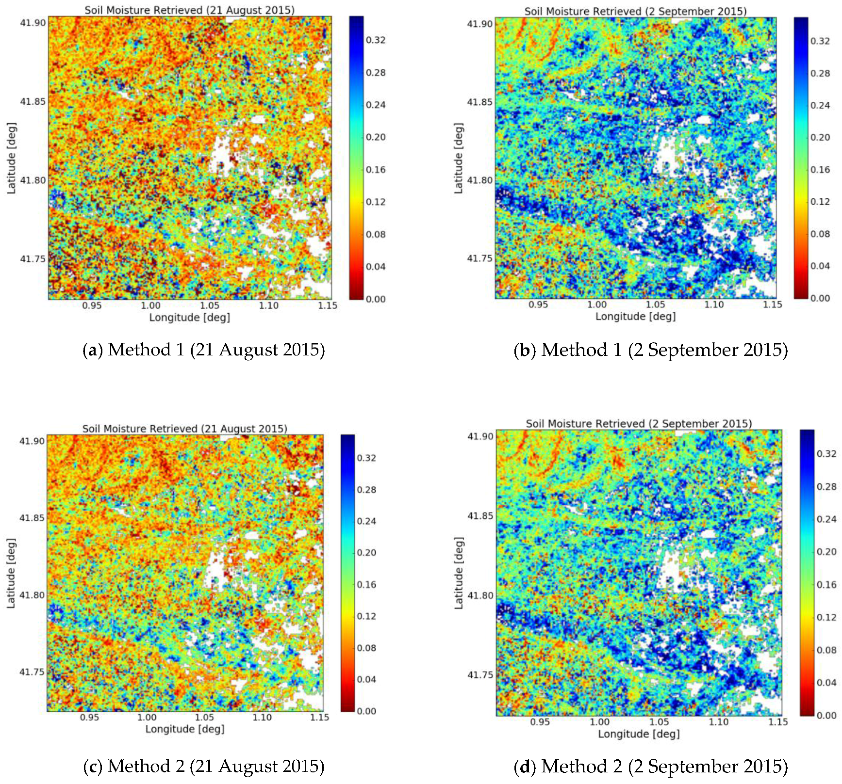
Figure 13.
Difference of soil moisture retrieved by method 2 and 1 for date 1 (21 August 2015) and date 2 (2 September 2015).
Figure 13.
Difference of soil moisture retrieved by method 2 and 1 for date 1 (21 August 2015) and date 2 (2 September 2015).
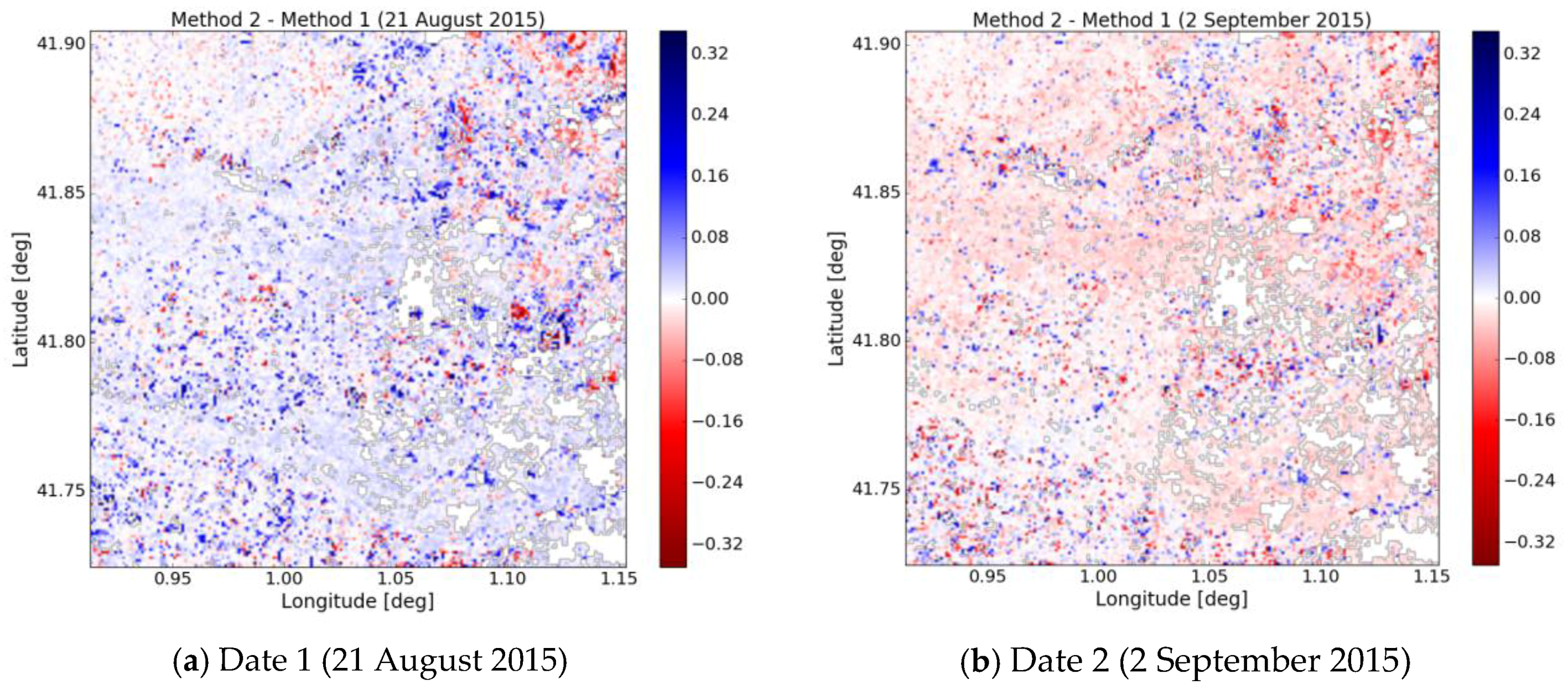
Figure 14.
RMS between methods 1 and 2, as a function of NDVI for date 21 August 2015 (a) and date 2 September 2015 (b).
Figure 14.
RMS between methods 1 and 2, as a function of NDVI for date 21 August 2015 (a) and date 2 September 2015 (b).


Table 1.
Ground soil moisture measurements in two demonstration fields at Foradada and Agramunt.
| Site | Foradada | Agramunt |
|---|---|---|
| Coordinates | 41.866° N, 1.015° E | 41.782° N, 1.089° E |
| At soil depths in cm | 3, 9, 10, 20 | 5, 10, 20, 40 |
| Period of ground measurements | May–August 2015 February–October 2016 | June–October 2015 July–November 2016 |
| Sand, silt, clay in % | 41.5, 42.3, 16.2 | 52.1, 35.3, 12.6 |
| Irrigation method | Sprinklers | Subsurface drippers |
| Surface soil moisture (min, max) in m3/m3 | (0.08, 0.45) | (0.04, 0.28) |
| Meteorological station | Baldomar station | Tornabous station |
Table 2.
Sentinel-1 database.
| Date | Date | Date | Date | Date | Date |
|---|---|---|---|---|---|
| 16 July 2015 | 13 Nov. 2015 | 05 Feb. 2016 | 29 Apr. 2016 | 03 Aug. 2016 | 26 Oct. 2016 |
| 28 July 2015 | 25 Nov. 2015 | 17 Feb. 2016 | 11 May 2016 | 15 Aug. 2016 | 07 Nov. 2016 |
| 09 Aug. 2015 | 07 Dec. 2015 | 29 Feb. 2016 | 23 May 2016 | 27 Aug. 2016 | 19 Nov. 2016 |
| 21Aug. 2015 | 19 Dec. 2015 | 12 Mar. 2016 | 04 June 2016 | 08 Sept. 2016 | - |
| 02 Sept. 2015 | 31 Dec. 2015 | 24 Mar. 2016 | 28 June 2016 | 20 Sept. 2016 | - |
| 14 Sept. 2015 | 12 Jan. 2016 | 05 Apr. 2016 | 10 July 2016 | 02 Oct. 2016 | - |
| 26 Sept.2015 | 24 Jan. 2016 | 17 Apr. 2016 | 22 July 2016 | 14 Oct. 2016 | - |
Table 3.
Sentinel-2 database.
| Date | Date | Date | Date | Date | Date | ||||
|---|---|---|---|---|---|---|---|---|---|
| 06 July 2015 | 21 Oct. 2015 | 19 Mar. 2016 | 21 May 2016 | 30 July 2016 | 28 Sept. 2016 | ||||
| 16 July 2015 | 20 Nov. 2015 | 22 Mar. 2016 | 28 May 2016 | 06 Aug. 2016 | 05 Oct. 2016 | ||||
| 02 Aug. 2015 | 30 Nov. 2015 | 29 Mar. 2016 | 07 June 2016 | 09 Aug. 2016 | 15 Oct. 2016 | ||||
| 05 Aug. 2015 | 03 Dec. 2015 | 01 Apr. 2016 | 10 June 2016 | 16 Aug. 2016 | 18 Oct. 2016 | ||||
| 12 Aug. 2015 | 23 Dec. 2015 | 08 Apr. 2016 | 20 June 2016 | 19 Aug. 2016 | 25 Oct. 2016 | ||||
| 15 Aug. 2015 | 30 Dec. 2015 | 11 Apr. 2016 | 27 June 2016 | 26 Aug. 2016 | 28 Oct. 2016 | ||||
| 22 Aug. 2015 | 12 Jan. 2016 | 18 Apr. 2016 | 30 June 2016 | 29 Aug. 2016 | 04 Nov. 2016 | ||||
| 25 Aug. 2015 | 19 Jan. 2016 | 28 Apr. 2016 | 07 July 2016 | 05 Sept. 2016 | 07 Nov. 2016 | ||||
| 11 Sept. 2015 | 29 Jan. 2016 | 01 May 2016 | 10 July 2016 | 08 Sept. 2016 | 14 Nov. 2016 | ||||
| 14 Sept. 2015 | 18 Feb. 2016 | 08 May 2016 | 17 July 2016 | 15 Sept. 2016 | 17 Nov. 2016 | ||||
| 24 Sept. 2015 | 09 Mar. 2016 | 11 May 2016 | 20 July 2016 | 18 Sept. 2016 | 24 Nov. 2016 | ||||
| 01 Oct. 2015 | 12 Mar. 2016 | 18 May 2016 | 27 July 2016 | 25 Sept. 2016 | 27 Nov. 2016 | ||||
© 2017 by the authors. Licensee MDPI, Basel, Switzerland. This article is an open access article distributed under the terms and conditions of the Creative Commons Attribution (CC BY) license (http://creativecommons.org/licenses/by/4.0/).
Share and Cite
MDPI and ACS Style
Gao, Q.; Zribi, M.; Escorihuela, M.J.; Baghdadi, N. Synergetic Use of Sentinel-1 and Sentinel-2 Data for Soil Moisture Mapping at 100 m Resolution. Sensors 2017, 17, 1966. https://doi.org/10.3390/s17091966
AMA Style
Gao Q, Zribi M, Escorihuela MJ, Baghdadi N. Synergetic Use of Sentinel-1 and Sentinel-2 Data for Soil Moisture Mapping at 100 m Resolution. Sensors. 2017; 17(9):1966. https://doi.org/10.3390/s17091966
Chicago/Turabian StyleGao, Qi, Mehrez Zribi, Maria Jose Escorihuela, and Nicolas Baghdadi. 2017. "Synergetic Use of Sentinel-1 and Sentinel-2 Data for Soil Moisture Mapping at 100 m Resolution" Sensors 17, no. 9: 1966. https://doi.org/10.3390/s17091966
Note that from the first issue of 2016, this journal uses article numbers instead of page numbers. See further details here.