Sliding Spotlight Mode Imaging with GF-3 Spaceborne SAR Sensor


1
Beijing Key Laboratory of Embedded Real-time Information Processing Technology, School of Information and Electronics, Beijing Institute of Technology, Beijing 100081, China
2
China Academy of Space Technology, Beijing Institute of Space System Engineering, Beijing 100086, China
*
Author to whom correspondence should be addressed.
Sensors 2018, 18(1), 43; https://doi.org/10.3390/s18010043
Submission received: 1 November 2017
/
Revised: 21 December 2017
/
Accepted: 22 December 2017
/
Published: 26 December 2017
(This article belongs to the Special Issue First Experiences with Chinese Gaofen-3 SAR Sensor)
Abstract
:Synthetic aperture radar (SAR) sliding spotlight work mode can achieve high resolutions and wide swath (HRWS) simultaneously by steering the radar antenna beam. This paper aims to obtain well focused images using sliding spotlight mode with the Chinese Gaofen-3 SAR sensor. We proposed an integrated imaging scheme with sliding spotlight echoes. In the imaging scheme, the two-step approach is applied to the spaceborne sliding spotlight SAR imaging algorithm, followed by the Doppler parameter estimation algorithm. The azimuth spectral folding phenomenon is overcome by the two-step approach. The results demonstrate a high Doppler parameter estimation accuracy. The proposed imaging process is accurate and highly efficient for sliding spotlight SAR mode.
1. Introduction
Stripmap mode can achieve wide swath imaging with the azimuth resolution below a half of azimuth antenna length [1]. Spotlight mode is characterized by azimuth antenna steering to a rotation center, which can achieve high azimuth resolution and a narrow swath. Sliding spotlight mode is characterized by azimuth antenna steering to a virtual rotation center during the raw data acquisition interval. With the control of the beam rotation rate and raw data acquisition interval, high resolutions and wide swath observation can be achieved simultaneously. In other words, sliding spotlight mode is the trade-off between stripmap mode and spotlight mode.
The feasibility of spotlight was verified by several satellites like Radarsat-2 [2], Cosmo-Skymed [3,4], ALOS-2 [5], TerraSAR-X [6,7], and Sentinel-1 [8], as well as the next generation SAR satellites such as TerraSAR Next Generation (TerraSAR-NG) [9,10]. The sliding spotlight mode in TerraSAR-X [11] applies a slower antenna steering than staring spotlight mode. The launch of the Chinese satellite Gaofen-3 in 2016 is the first C-band and high-resolution, fully polarimetric SAR satellite with 12 imaging modes, including sliding spotlight mode [12,13,14]. Different from traditional stripmap SAR, signal processing of sliding spotlight echoes faces several difficulties. First, the total Doppler bandwidth exceeds Pluse Reputation Frequency (PRF), and the spectrum aliasing must be solved. Second, for the resolution is high in sliding spotlight imaging, and the Doppler parameter must be acquired accurately either via orbit parameters in the WGS-84 coordinates system or Doppler parameter estimation.
Various algorithms used to overcome spectrum aliasing have been proposed in recent years [15,16,17,18,19,20]. The classical two-step imaging algorithm is introduced to overcome the azimuth spectrum aliasing [15,16]. Sub-aperture algorithms are another way to deal with the azimuth spectrum aliasing [17], whereas the sub-aperture algorithms need sub-aperture formation, which is not efficient due to azimuth data overlap. Furthermore, a new algorithm named baseband azimuth scaling (BAS) is proposed for both TOPS (Terrain Observation by Progressive Scans) and sliding spotlight data imaging [6,18,19]. But the sub-aperture number in BAS algorithm may be large while the processed azimuth bandwidth is close to PRF. These methods can overcome spectrum aliasing and achieve sliding spotlight imaging. However, the Doppler parameter estimation methods are required to combine with the imaging algorithm due to the high-resolution imaging.
In principle, it is possible to calculate the Doppler parameter from orbit and attitude data, but measurement uncertainties on these parameters will limit the accuracy. In order to obtain the accurate Doppler parameter, a lot of Doppler parameter estimation methods are proposed in recent years. The Doppler centroid can be estimated by [21,22,23,24]. References [21,22] propose Doppler centroid estimation algorithm using azimuth spectrum and antenna pattern, which are kinds of frequency algorithm. The proposed algorithm in references [23,24] is a time domain algorithm and denoted the correlation Doppler estimator with high efficiency. However, these methods are suitable for Doppler centroid estimation in stripmap mode since the PRF is slightly above the Doppler bandwidth. Azimuth antenna steering in sliding spotlight leads to the variation of the Doppler centroid in azimuth, and the Doppler bandwidth exceeds PRF, which cannot be applied in traditional Doppler centroid method.
The Doppler frequency rate is one of the key parameters in the azimuth focusing of SAR data. Once mismatched, it will cause serious defocusing in azimuth direction and result in the degradations of image quality. Several Doppler frequency rate estimation algorithms [25,26,27,28,29,30] are proposed including the Map Drift (MD) [25,26], phase gradient autofocus (PGA) [27,28] and contrast optimization algorithm [29] with high accuracy. However, since different azimuth targets share different time support domains and different frequency support domains in sliding-spotlight mode, the MD algorithm cannot be applied as the Doppler frequency rate estimation algorithm. Also, the PGA algorithm cannot be applied in the sliding spotlight working mode directly since different azimuth targets share different time support domain, which is different from spotlight mode. In this paper, contrast optimization algorithm is introduced and adopted as Doppler frequency rate estimation.
In this paper, we proposed an integrated imaging scheme with sliding spotlight mode. In the imaging scheme, the two-step approach is firstly applied to the spaceborne sliding spotlight SAR imaging algorithm, followed by the modified correlation Doppler centroid estimator and modified contrast optimization algorithm. The azimuth spectral fol algorithm ding phenomenon is overcome by the two-step approach, and the chirp scaling (CS) [1] algorithm is applied to obtain the unambiguous images. The Doppler centroid variation along azimuth can be estimated by modified correlation Doppler estimator with high accuracy. The Doppler frequency rate variation along range can be estimated by contrast optimization algorithm with high accuracy. The proposed imaging process is accurate and efficient for sliding spotlight SAR mode.
2. Gaofen-3 Sliding Spotlight Mode and Signal Characteristics Analysis
2.1. Gaofen-3 Sliding Spotlight Mode and Imaging Geometry
Sliding Spotlight mode is the highest resolution observation mode in this Chinese Gaofen-3 SAR sensor. This imaging mode provides 1 m resolution with 10 km swath width.
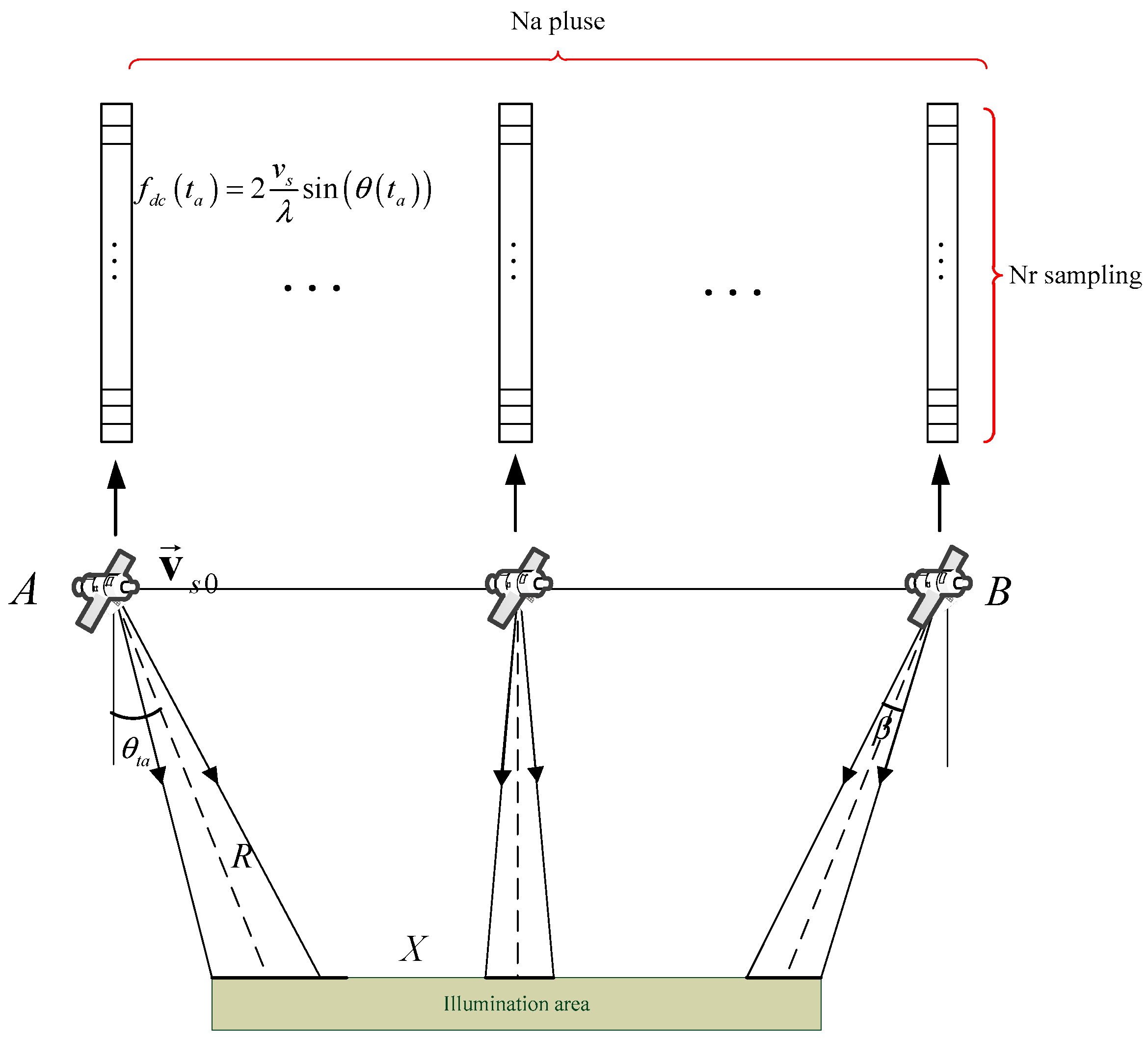
The planar imaging geometry of the sliding-spotlight mode is shown in Figure 1, which is simplified by linear geometry since the azimuth rotation angle is small enough. In the sliding spotlight imaging geometry, the azimuth beam steers from fore to aft at a constant rotation rate as
where is the instantaneous squint angle and is the whole acquisition interval, and and are the slant ranges from the flight path to the scene center and the virtual rotation center to the scene center, respectively. is the virtual rotation center, is the azimuth beam width, is the width in the azimuth direction.
For azimuth beam scanning at a constant rotation rate leading to , the steering factor is defined as [29]
Then compared with stripmap working mode, the azimuth resolution of the sliding-spotlight mode is improved by the factor as , where is the azimuth antenna length.
2.2. Properties of the Echo Signal and Imaging Algorithm Consideration
While the transmitter illuminates the target scene with a baseband chirp signal and a point target locates at , the echo of transmitted pulse can be expressed as
where is the wavelength, is the FM (frequency modulation) rate. is the footprint velocity taking into account azimuth beam steering. and are fast time and slow time variables, respectively. Based on rectilinear imaging geometry of sliding-spotlight mode, can be written as
where is the effective velocity which is usually used for the imaging focus.
Because of the Range Doppler (RD) [1], CS and nonlinear CS (NCS) [31,32] algorithms are all high efficient frequency imaging algorithm without interpolation, and one of the imaging algorithm is adopted in the Gaofen-3 sliding spotlight processing. In the RDA, the difference of range cell migration (RCM) in the whole scene is assumed as 0, which leads to the RCM error [33]
where is the RCM difference between near range and far range margin in the scene, is the swath width. The is equal to 0.96 m while , and , which is larger than range resolution. Thus, RDA cannot be applied in Gaofen-3 sliding spotlight imaging for the RCM error in RDA cannot be neglect. The major error in CS algorithm (CSA) including two parts: one is the variation of along the range direction, which leads to RCM error, and another is the variation of in range-Doppler domain, which is assumed not related to range [1], where can be expressed as
where .
Firstly, the effective velocity slightly varies with range. In the typical Gaofen-3 orbit, varies 2 m/s in 10 km swath. Thus, the RCM error caused by is independent of the range direction and can be expressed as
As shown in Figure 2, the varies with , the maximum of is equal to −0.13 m while , and , which is much smaller than range resolution.
Secondly, the error caused by it varies with is calculated by
In essential, this error is the variation of second range compression (SRC) in range time domain which cannot be compensated in CS algorithm. The variation between SRC error and range frequency is presented in Figure 3. Notice in Equation (8) is chosen as maximum of Doppler bandwidth. The maximum of is equal to 0.3 rad, which is smaller than . As a result, the CS algorithm is accurate and efficient enough for sliding spotlight SAR imaging in Gaofen-3.
3. Processing Overview
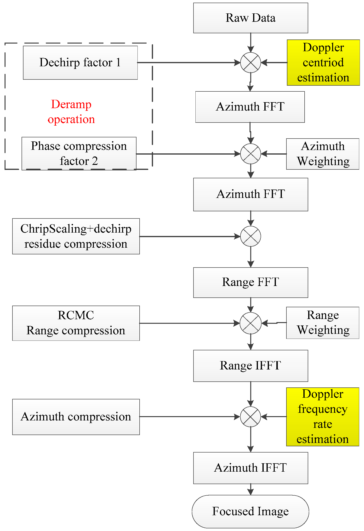
In this section, based on CSA, we propose a complete process of sliding spotlight imaging with Doppler parameter estimation. Figure 4 is the processing flow of the Gaofen-3 sliding spotlight mode.
From Figure 4, three techniques are vital for obtaining focused images: Deramp operation, Doppler centroid estimation, and Doppler frequency rate estimation. As Figure 4 shows, the Doppler centroid estimation and Doppler frequency rate estimation are the main contributions of this paper.
3.1. Azimuth Preprocessing in Sliding Spotlight Mode
In general, the total Doppler bandwidth is larger than the PRF in the sliding spotlight mode. In order to overcome the aliasing of the azimuth echo in the frequency domain, azimuth convolution processing is conducted, which is the key point of azimuth preprocessing. The quadratic phase signal is expressed as
where is the variation rate and is the physical velocity of the SAR sensor.
While conducting the azimuth weighting processing, the azimuth preprocessing can be accomplished by employing
Substituting Equation (9) into Equation (10), Equation (10) can be rewritten as
From Equation (11), the azimuth convolution processing includes three parts: dechirp processing, Fourier transform, and residue compensation.
3.2. The Estimation of Doppler Centroid in Sliding Spotlight Mode
A lot of Doppler centroid estimation algorithms are developed in SAR imaging. The proposed algorithm in reference [23] is denoted the correlation Doppler estimator (CDE) with high efficient. However, the CDE cannot be used in sliding spotlight mode since the Doppler bandwidth exceeds PRF. Based on CDE in [23], a modified CDE is developed that can be used to estimate the variation of Doppler centroid in azimuth.
Based on the fact that the echo in PRT is related to the echo in PRT and the correlation is strongest when . Thus, is adopted in the following experiments. Notice in Equation (13), the summation should not be along the azimuth direction since the azimuth beam steering leads to the variation of , which should be estimated. To improve the accuracy in low SNR condition, taking the average in range is necessary and helpful. Therefore, the variation of in range direction is neglected, which leads to a small error about several hertz. The variation of in range direction will be discussed below.
Because the in azimuth beam steering may be greater than PRF, Doppler ambiguity occurs. Fortunately, the sliding spotlight mode in GF-3 is not squinted SAR, and thus the Doppler ambiguity number in azimuth reference time is 0. Therefore, the Doppler ambiguity that can be calculated for the PRF is known, and the variation along azimuth time is obtained.
Since the is estimated by raw data, the relationship between geometry and estimated by raw data is shown in Figure 5. In Figure 5, the estimated by raw data at each azimuth is expressed by
where is squint angle and varies along with azimuth time. Although the in azimuth time relates to the targets located in the beam direction and the target in the beam width, the is just the equation of .
If the variation along range is required, one can calculate the variation using the orbit and satellite attitude parameters. Although some small deviation exists in these parameters, the variation along range is accurate enough since it is small and the tendency of can be calculated accurately.
In Ref. [23], the azimuth slow time delay for autocorrelation function goes rapidly to zero with increasing. However, the azimuth Doppler bandwidth of a single target is larger than PRF. Thus, under the condition of , the Cramer-Rao Bound (CRB) on the estimation method in sliding spotlight mode can be deduced from the interferometic phase , i.e.,
where is the accumulation number, is the CRB of the interferometic phase and is the coherence between the azimuth echo and , where
3.3. The Estimation of Doppler Frequency Modulation Rate in Sliding Spotlight Mode
After range compression, the Doppler frequency modulation rate is required in azimuth compression. The contrast optimization algorithm [29] is adopted in imaging algorithm. For azimuth compression function can be expressed as
we estimate directly using the Equation (17). The contrast is defined as [29]
where represents the range sampling point.
In some special cases, autofocus may fail in a few range sampling positions. To solve this problem, one can adopt the mean value between the autofocus failure sampling positions. Finally, linear fitting between slant range and is carried out and the fitting coefficient is used in azimuth focusing.
4. Experimental Results
In this section, the estimation of Doppler parameters including Doppler centroid and Doppler frequency modulation rate are demonstrated, followed by the focus images. The parameters of Gaofen-3 sliding spotlight mode are list in Table 1. Here, we choose two typical scenes for Doppler parameter estimation. Scene 1 is the border region between the land and the large-scale sea area, scene 2 is a mountainous area.
4.1. The Estimation of Doppler Centroid Using GF-3 Real Data
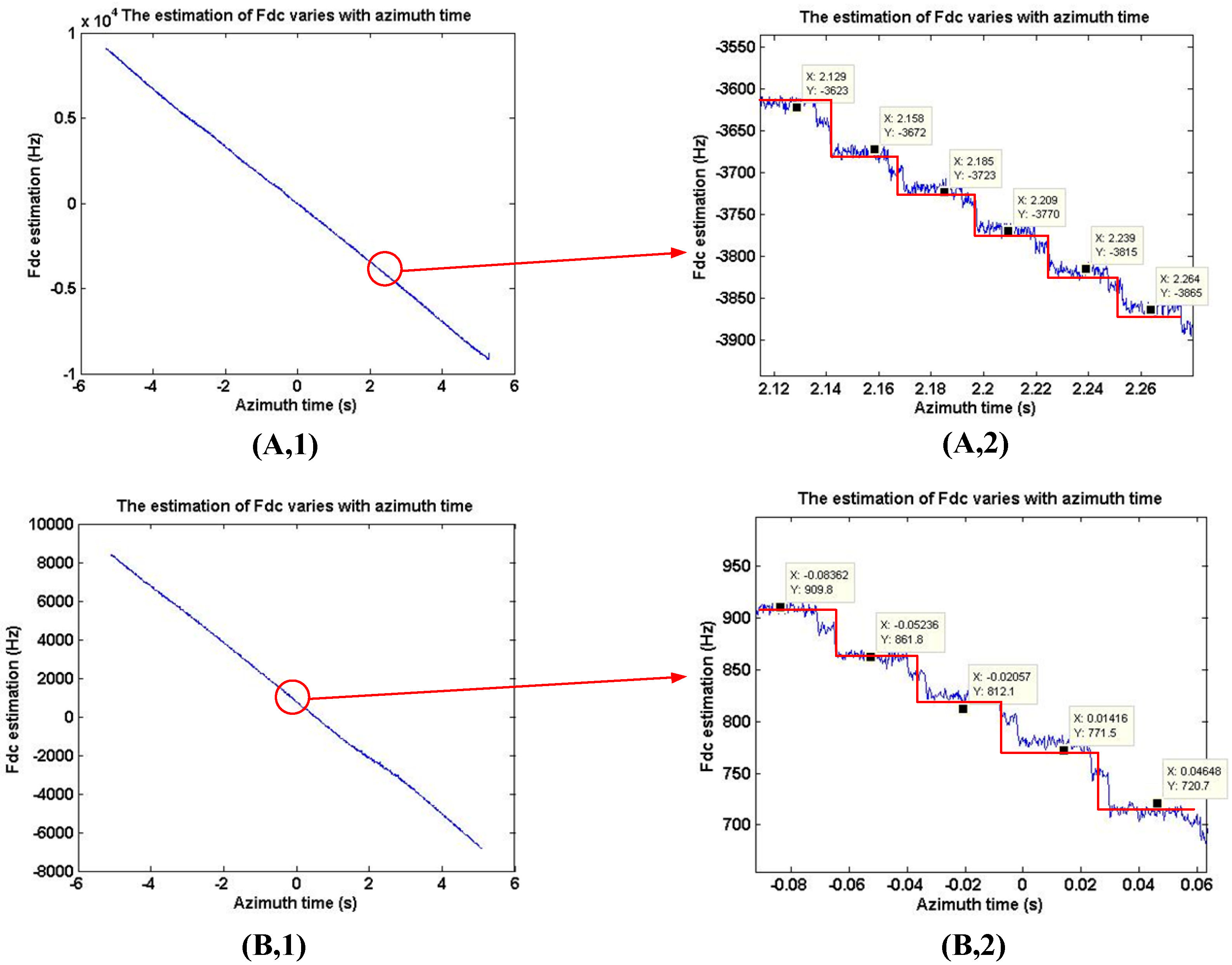
The experiments of Doppler centroid estimation include two parts. First, neglecting the variation of in range direction, the estimation in azimuth direction is shown in Figure 6. The active phased array antenna is adopted in Gaofen-3 SAR sensor, which can achieve electronic scanning in azimuth direction. In scenes 1 and 2, the variation in azimuth are equal to 18,000 Hz and 15,320 Hz for the azimuth rotation angle are equal to 3.8° and 3.22°, respectively, which are nearly equal to the estimation shown in Figure 6. Because the azimuth electronic scanning is not continuous and the azimuth beam scanning step in these image are 0.01°, the variation is not continuous, and the step is equal to 48 Hz. In Figure 6, the variation in azimuth is like step and measured approximately equal to 48 Hz, thus estimation accuracy in the Doppler centroid estimation method is verified by different scene in Gaofen-3 sliding spotlight imaging.
Second, to calculate the varies with range direction, the orbit and satellite attitude parameters are used, and the variation is . Thus, the variation in the whole scene is obtained.
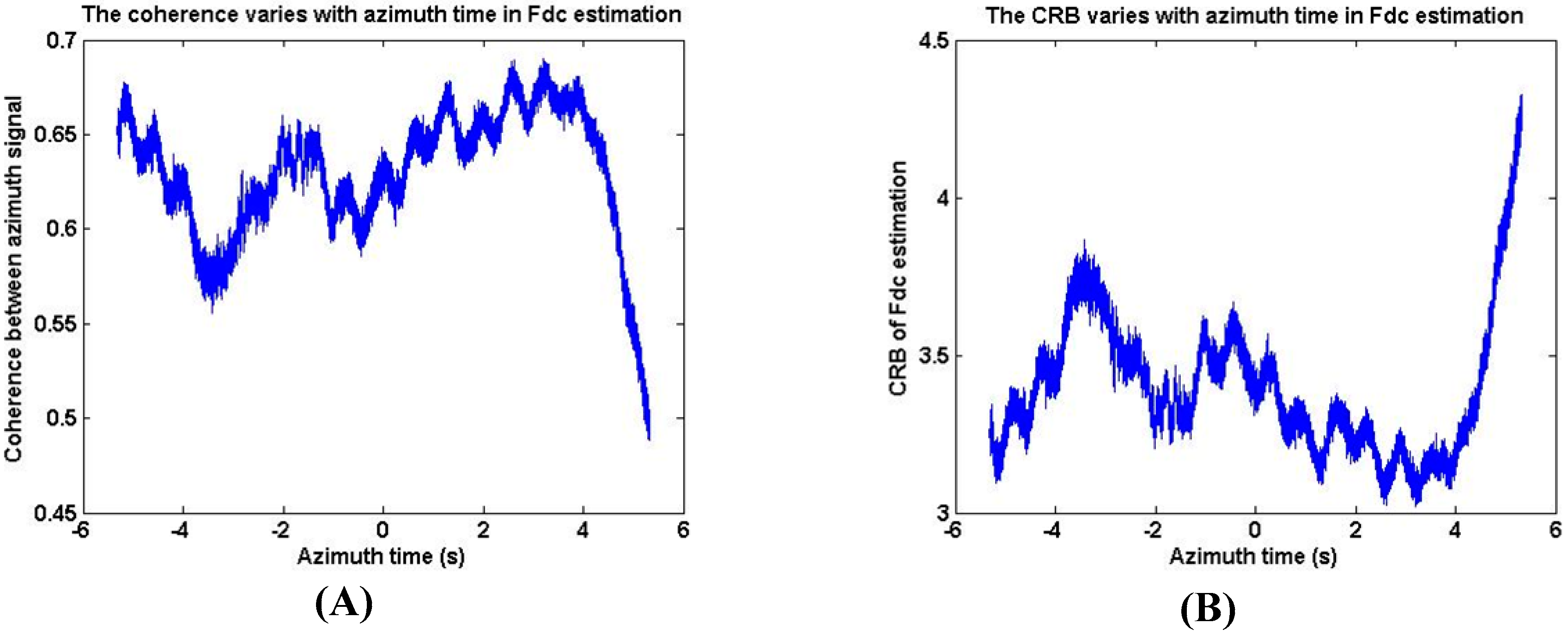
Third, based on scene 1 data, the CRB of the estimation method is demonstrated in Figure 7. As Figure 7 shows, the coherence in estimation is between 0.5 and 0.7 and the CRB of estimation is below 5, which means the theoretical accuracy is high enough although the Doppler bandwidth is larger than PRF in Gaofen-3 sliding spotlight mode.
4.2. The Estimation of Doppler Frequency Modulation Rate Using GF-3 Real Data
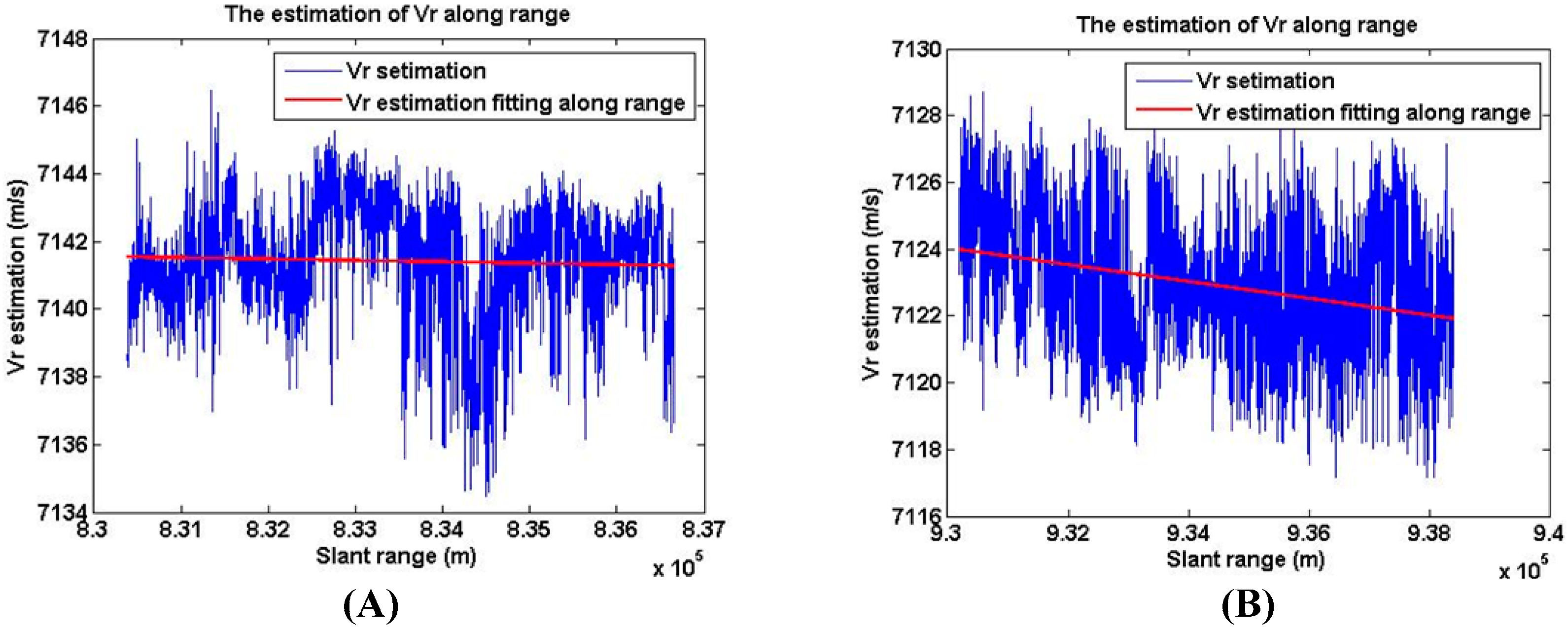
Based on the contrast optimization algorithm, the estimation of along range is demonstrated in Figure 8. As Figure 8 shows, the variation of along range is about 2 m/s in 10 km swath, which is close to the theoretical value.
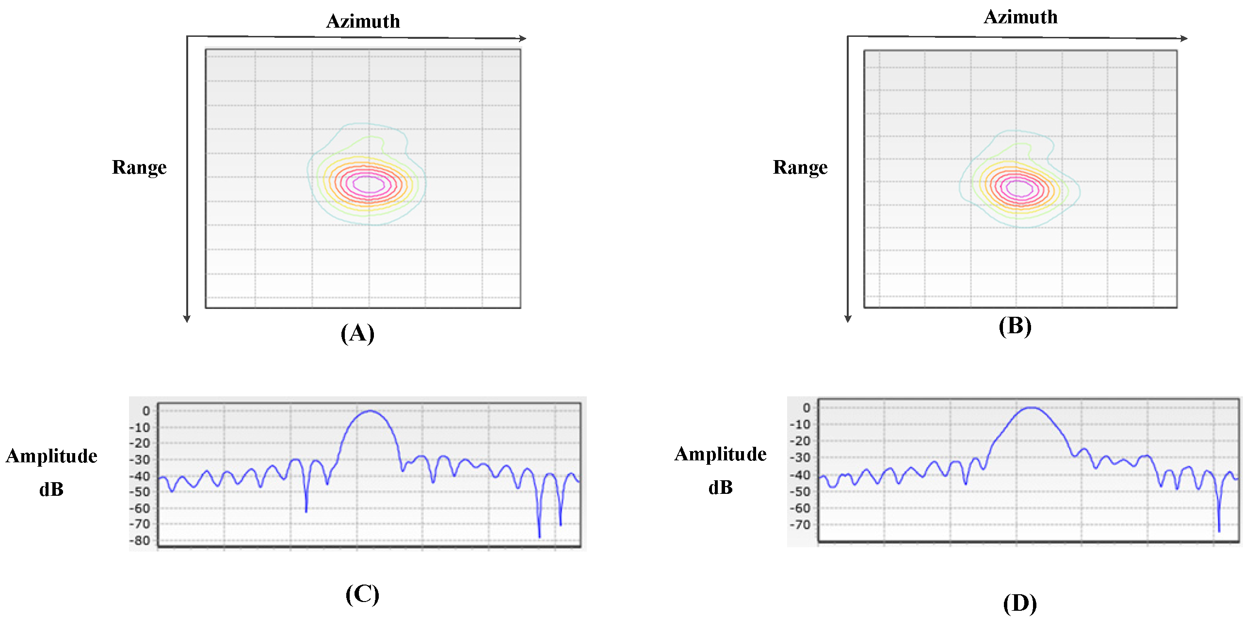
In order to show the improvement of image quality by proposed Doppler parameter estimation method, a point target is analyzed in detail. Using the estimated by the contrast optimization algorithm and the estimated by modified CDE to finish azimuth compression, the images are well focused and shown in Figure 9. Figure 10 shows the images focusing by orbit and satellite attitude parameters. Comparing Figure 9 with Figure 10, one can find the target in Figure 10 is defocus while the target in Figure 9 is well focused. To evaluate the performance of the focused target, the target (1) is chosen and the 2-D focused images and the slices in azimuth are presented in Figure 11. The peak side lobe ratio (PSLR) and integrated side lobe ratio (ISLR) and resolutions of the point targets are given in Table 2. Obviously, calculating Doppler parameter by orbit and satellite attitude parameters results a small bias, which can lead to defocus. However, with the help of proposed Doppler parameter estimation method, the focus performance is close to theoretical value. Thus, the contrast optimization algorithm is verified by the Gaofen-3 sliding spotlight data.
5. Conclusions
This paper proposes an integrated sliding spotlight imaging scheme for Chinese Gaofen-3 SAR sensor. The focused imaging relies on the two-step approach and Doppler parameter estimation accuracy. The two-step approach is effective and highly efficient in sliding spotlight imaging. Moreover, the modified CDE is accurate enough because it can offer the Doppler centroid in every azimuth sampling time. The estimation of the Doppler frequency modulation rate can achieve high accuracy, and the point target of real SAR data in Gaofen-3 is evaluated.
Acknowledgments
This work was supported by the National Natural Science Foundation of China under Grant No. 61370017, 61225005, 61120106004 and the China High Resolution Earth Observation System Project under Grant No. 41-Y20A13-9001-15/16, 12-Y20A15-9001-15/16.
Author Contributions
Qingjun Zhang conceived the idea; Feng Xiao designed and conducted the experiments; Zegang Ding analyzed the data; Meng Ke wrote the paper; Tao Zeng supervised the research, including the experiments and development.
Conflicts of Interest
The authors declare no conflict of interest.
References
- Cumming, I.G.; Wong, F.H. Digital Processing of Synthetic Aperture Radar Data: Algorithms and Implementation; Artech House: Norwood, MA, USA, 2005. [Google Scholar]
- Brule, L.; Baeggli, H. Radarsat-2 program update. In Proceedings of the IEEE International Geoscience and Remote Sensing Symposium (IGARSS), Toronto, ON, Canada, 24–28 June 2002; pp. 1462–1464. [Google Scholar]
- Caltagirone, F.; Spera, P.; Vigliotti, R.; Manoni, G. Skymed/COSMO mission overview. In Proceedings of the IEEE International Geoscience and Remote Sensing Symposium (IGARSS), Seattle, WA, USA, 6–10 July 1998; Volume 2, pp. 683–685. [Google Scholar]
- Lorusso, R.; Nicoletti, M.; Gallipoli, A.; Lorè, V.A.; Milillo, G.; Lombardi, N.; Nirchio, F. Extension of Wavenumber Domain Focusing for spotlight COSMO-SkyMed SAR Data. Eur. J. Remote Sens. 2015, 48, 49–70. [Google Scholar] [CrossRef]
- Shimada, M. Alos-2 science program. In Proceedings of the IEEE International Geoscience and Remote Sensing Symposium (IGARSS), Meibourne, Australia, 21–26 July 2013; pp. 2400–2403. [Google Scholar]
- Breit, H.; Fritz, T.; Balss, U.; Lachaise, M.; Niedermeier, A.; Vonavka, M. Terrasar-x SAR processing and products. IEEE Trans. Geosci. Remote Sens. 2010, 48, 727–740. [Google Scholar] [CrossRef]
- Pitz, W.; Miller, D. The TerraSAR-X satellite. IEEE Trans. Geosci. Remote Sens. 2010, 48, 615–622. [Google Scholar] [CrossRef]
- Scheiber, R.; Wollstadt, S.; Sauer, S.; Malz, E. Sentinel-1 imaging performance verification with TerraSAR-X. In Proceedings of the 2010 8th European Conference on Synthetic Aperture Radar (EUSAR), Aachen, Germany, 7–10 June 2010; pp. 55–58. [Google Scholar]
- Janoth, J.; Gantert, S.; Schrage, T.; Kaptein, A. TerraSAR next generation—Mission capabilities. In Proceedings of the IEEE International Geoscience and Remote Sensing Symposium (IGARSS), Melbourne, Australia, 21–26 July 2013; pp. 2297–2300. [Google Scholar]
- Gantert, S.; Kern, A.; Düring, R.; Janoth, J.; Petersen, L.; Herrmann, J. The future of X-band SAR: TerraSAR-X next generation and worldSAR constellation. In Proceedings of the 2013 Asia-Pacific Conference on Synthetic Aperture Radar (APSAR), Tsukuba, Japan, 23–27 September 2013; pp. 20–23. [Google Scholar]
- Blecher, D.P.; Baker, C.J. High resolution processing of hybrid strip-map/spotlight mode SAR. IEE Proc. Radar Sonar Navig. 1996, 143, 366–374. [Google Scholar] [CrossRef]
- Zhang, Q.J. System design and key technologies of the GF-3 satellite. Acta Geod. Cartogr. Sin. 2017, 46, 269–277. [Google Scholar]
- Yun, F. GF-3 satellite. Satell. Appl. 2016, 8, 80. [Google Scholar]
- Sun, J.; Yu, W.; Deng, Y. The SAR Payload Design and Performance for the GF-3 Mission. Sensors 2017, 17, 2419. [Google Scholar] [CrossRef] [PubMed]
- Lanari, R.; Tesauro, M.; Sansosti, E.; Fornaro, G. Spotlight SAR Data Focusing Based on a Two-Step Processing Approach. IEEE Trans. Geosci. Remote Sens. 2001, 39, 1993–2003. [Google Scholar] [CrossRef]
- Liu, F.F.; Ding, Z.G.; Zeng, T.; Long, T. Performance Analysis of Two-Step Algorithm in Sliding Spotlight Space-borne SAR. In Proceedings of the IEEE Radar Conference, Arlington, TX, USA, 10–14 May 2010; pp. 965–968. [Google Scholar]
- Mittermayer, J.; Lord, R.; Borner, E. Sliding Spotlight SAR Processing for TerraSAR-X Using a New Formulation of the Extended Chirp Scaling Algorithm. In Proceedings of the IEEE International Geoscience and Remote Sensing Symposium(IGARSS), Toulouse, France, 21–25 July 2003; pp. 1462–1464. [Google Scholar]
- Prats, P.; Scheiber, R.; Mittermayer, J.; Meta, A.; Moreira, A. Processing of Sliding Spotlight and TOPS SAR Data Using Baseband Azimuth Scaling. IEEE Trans. Geosci. Remote Sens. 2010, 48, 770–780. [Google Scholar] [CrossRef] [Green Version]
- Wu, Y.; Sun, G.-C.; Yang, C.; Yang, J.; Xing, M.; Bao, Z. Processing of very high resolution spaceborne sliding spotlight SAR data using velocity scaling. IEEE Trans. Geosci. Remote Sens. 2016, 54, 1505–1518. [Google Scholar] [CrossRef]
- Yang, W.; Chen, J.; Liu, W.; Wang, P.; Li, C. A Modified Three-Step Algorithm for Tops and Sliding Spotlight SAR Data Processing. IEEE Trans. Geosci. Remote Sens. 2017, 55, 6910–6921. [Google Scholar] [CrossRef]
- McDonough, R.N.; Raff, B.E.; Kerr, J.L. Image formation from spaceborne synthetic aperture radar signals. Johns Hopkins APL Tech. Dig. 1985, 6, 300–312. [Google Scholar]
- Li, F.-K.; Held, D.N.; Curlander, J.C.; Wu, C. Doppler parameter estimation for spaceborne synthetic-aperture radars. IEEE Trans. Geosci. Remote Sens. 1985, 1, 47–56. [Google Scholar] [CrossRef]
- Madsen, S.N. Estimating the Doppler Centroid of SAR Data. IEEE Trans. Aerosp. Electron. Syst. 1989, 25, 134–140. [Google Scholar] [CrossRef] [Green Version]
- Li, J.; Li, X.; Lin, M.; Shi, J.; Zhang, S. Maximum-likelihood-based Doppler centroid estimation algorithm for MC-HRWS SAR system. Electron. Lett. 2014, 50, 1630–1631. [Google Scholar] [CrossRef]
- Curlander, J.C.; Wu, C.; Pang, A. Automated processing of spaceborne SAR data. In Proceedings of the IEEE International Geoscience and Remote Sensing Symposium (IGARSS), Munich, Germany, 1–4 June 1982; Volume 1, pp. 3–6. [Google Scholar]
- Ran, L.; Liu, Z.; Li, T.; Xie, R.; Zhang, L. Extension of Map-Drift Algorithm for Highly Squinted SAR Autofocus. IEEE J. Sel. Top. Appl. Earth Observ. Remote Sens. 2017, 10, 4032–4044. [Google Scholar] [CrossRef]
- Carrara, W.G.; Goodman, R.S.; Majewski, R.M. Spotlight Synthetic Aperture Radar: Signal Processing Algorithms; Artech House: Norwood, MA, USA, 1995. [Google Scholar]
- Jakowatz, C.V.; Wahl, D.E.; Eichel, P.H.; Ghiglia, D.C.; Thompson, P.A. Spotlight-Mode Synthetic Aperture Radar: A Signal Processing Approach; Kluwer Academic: Boston, MA, USA, 1996. [Google Scholar]
- Berizzi, F.; Corsini, G. Autofocusing of inverse synthetic aperture radar images using contrast optimization. IEEE Trans. Geosci. Remote Sens. 1996, 32, 1185–1191. [Google Scholar] [CrossRef]
- Yao, Y.; Song, W.; Ye, S. An Improved Autofocus Approach Based on 2-D Inverse Filtering for Airborne Spotlight SAR. In Proceedings of the 2016 CIE International Conference on Radar, Guangzhou, China, 10–13 October 2016. [Google Scholar]
- Davidson, G.W.; Cumming, I.G.; Ito, M.R. A Chirp Scaling Approach for Processing Squint Mode SAR Data. IEEE Trans. Aerosp. Electron. Syst. 1996, 32, 121–133. [Google Scholar] [CrossRef]
- An, D.X.; Huang, X.T.; Jin, T.; Zhou, Z.M. Extended Nonlinear Chirp Scaling Algorithm for High-Resolution Highly Squint SAR Data Focusing. IEEE Trans. Geosci. Remote Sens. 2012, 50, 3595–3609. [Google Scholar] [CrossRef]
- Bao, Z.; Xing, M.; Wang, T. Radar Imaging Technique; Electronics Industry: Beijing, China, 2005. [Google Scholar]
Figure 1.
Space-borne sliding-spotlight mode planar imaging earth geometry.
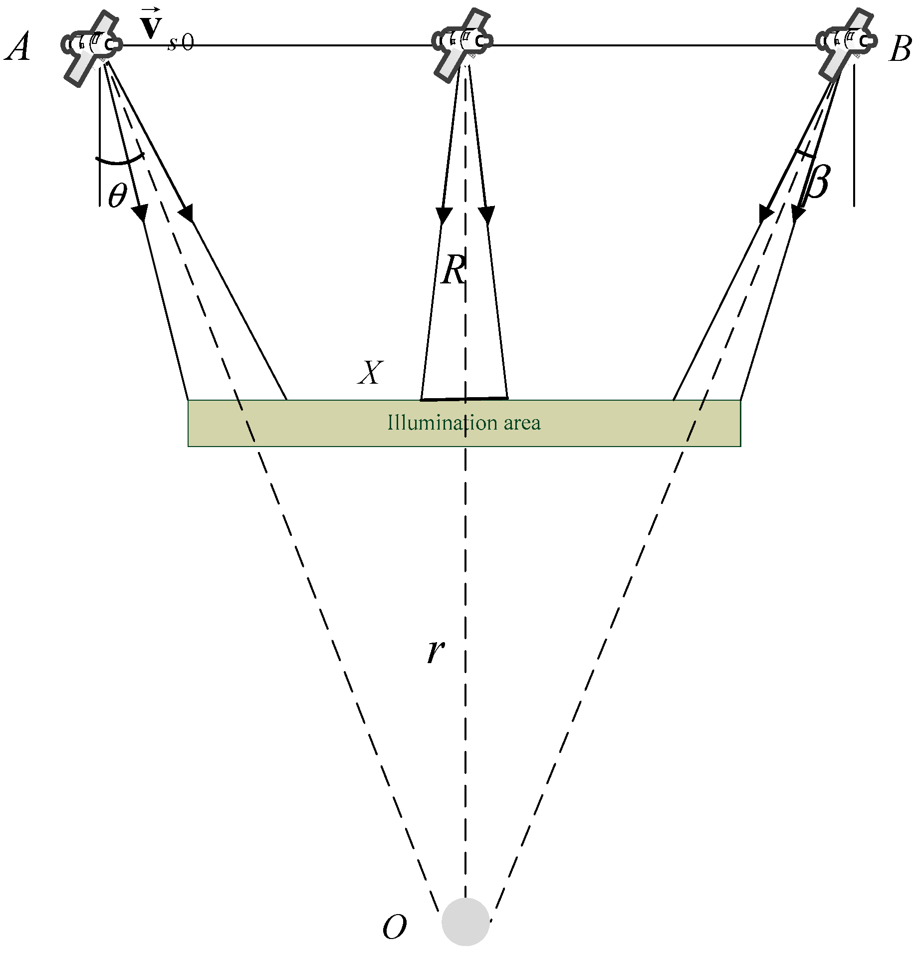
Figure 2.
The relationship between range cell migration (RCM) error in chirp scaling algorithm (CSA) and azimuth frequency. The RCM error is caused by the effective velocity slightly varying with range.
Figure 2.
The relationship between range cell migration (RCM) error in chirp scaling algorithm (CSA) and azimuth frequency. The RCM error is caused by the effective velocity slightly varying with range.
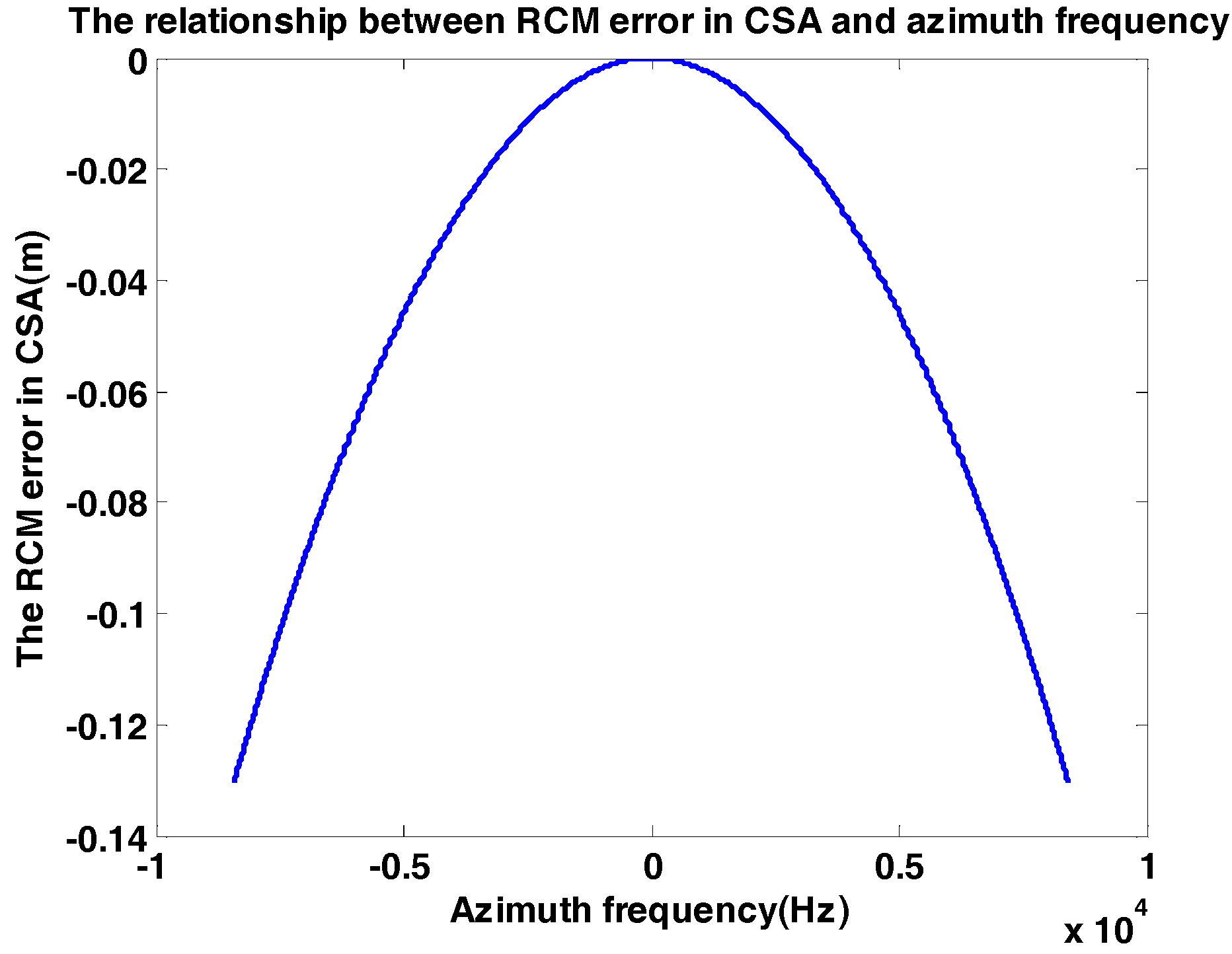
Figure 3.
The relationship between second range compression (SRC) error in CSA and range frequency. The SRC error is caused by variation in time domain.
Figure 3.
The relationship between second range compression (SRC) error in CSA and range frequency. The SRC error is caused by variation in time domain.
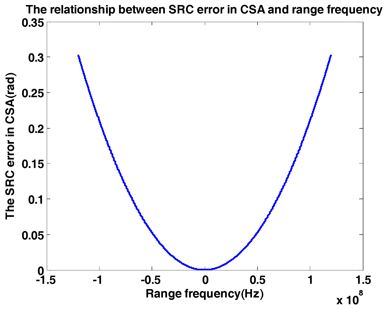
Figure 4.
Processing overview for Gaofen-3 sliding spotlight imaging. The main contributions of this paper are the Doppler centroid estimation and Doppler frequency rate estimation, which are shown in yellow box.
Figure 4.
Processing overview for Gaofen-3 sliding spotlight imaging. The main contributions of this paper are the Doppler centroid estimation and Doppler frequency rate estimation, which are shown in yellow box.

Figure 5.
The relationship between imaging geometry and estimated by raw data.

Figure 6.
The estimation of varies with azimuth time Gaofen-3 sliding spotlight images. (A,1) The estimation of varies with azimuth time in scene 1. (A,2) The enlargement of Figure (A,1). (B,1) The estimation of varies with azimuth time in scene 2. (B,2) The enlargement of Figure (B,1). The red line shows the step-like variation of .

Figure 7.
The CRB and Coherence in the estimation of varies with azimuth time. (A) The coherence in estimation. (B) The CRB of estimation.
Figure 7.
The CRB and Coherence in the estimation of varies with azimuth time. (A) The coherence in estimation. (B) The CRB of estimation.

Figure 8.
The estimation of along range in Gaofen-3 sliding spotlight images. (A) The estimation of along range in scene 1. (B) The estimation of along range in scene 2.
Figure 8.
The estimation of along range in Gaofen-3 sliding spotlight images. (A) The estimation of along range in scene 1. (B) The estimation of along range in scene 2.

Figure 9.
Gaofen-3 1 m resolution sliding spotlight images focusing by proposed Doppler parameter estimation method. (A) Scene 1: the border region between the land and the large-scale sea area. (B) Scene 2: the mountainous area. The strong scattering point is in the square and the enlarged view is beside the picture.
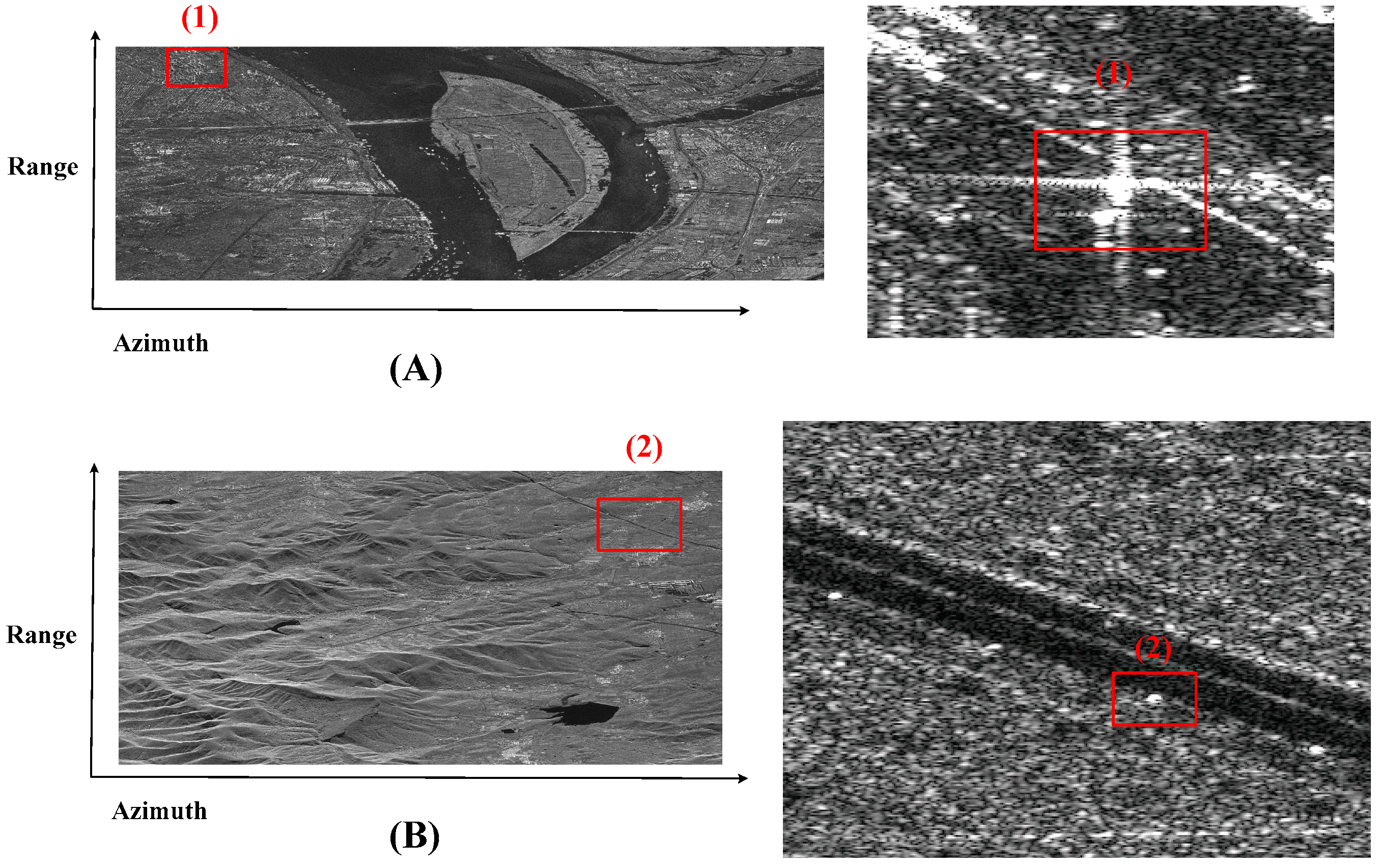
Figure 10.
Gaofen-3 1 m resolution sliding spotlight images focusing by orbit and satellite attitude parameters. (A) Scene 1: the border region between the land and the large-scale sea area. (B) Scene 2: the mountainous area. The strong scattering point is in the square and the enlarged view is beside the picture.
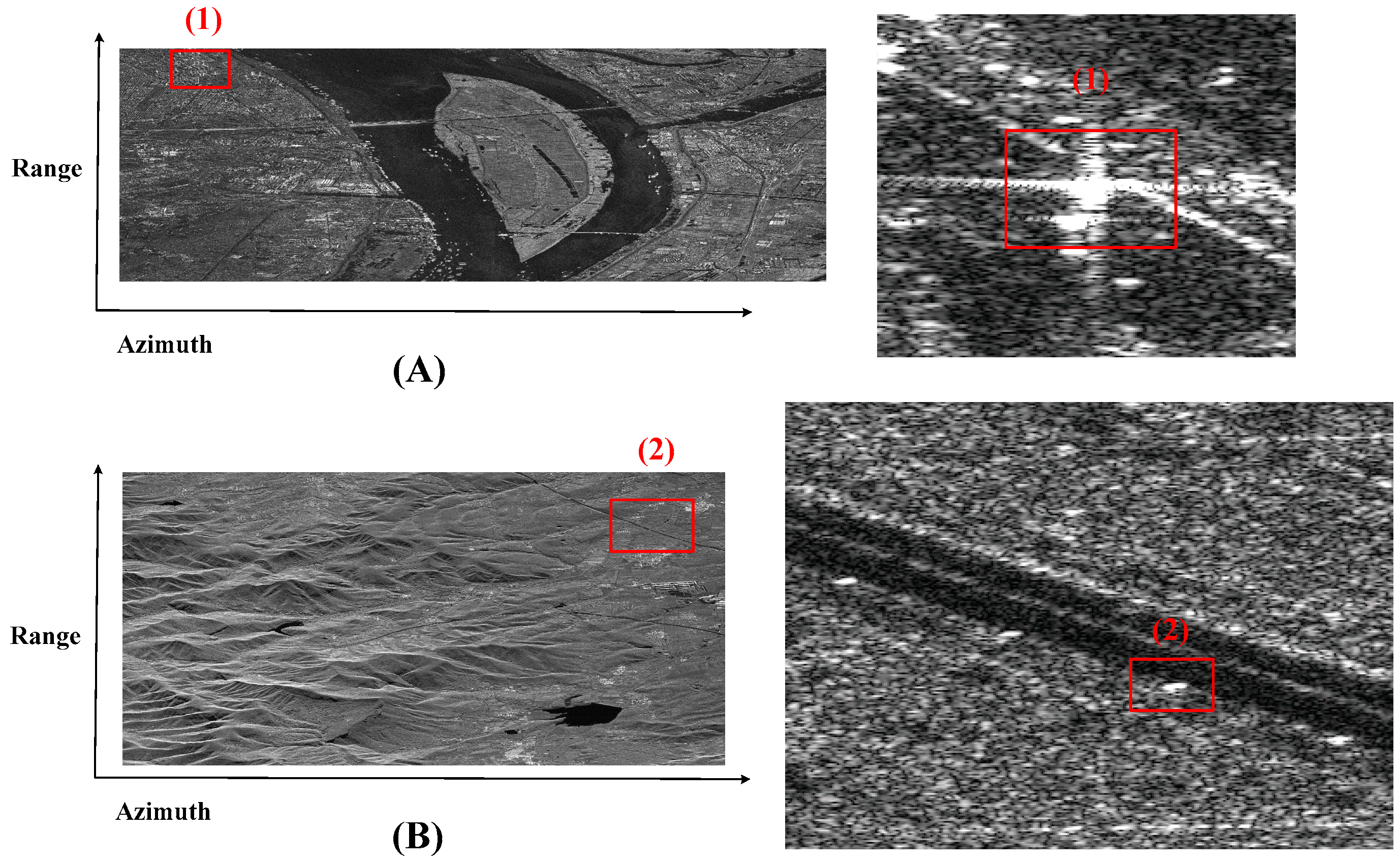
Figure 11.
The 2D focused image and the slices in azimuth of point target (1) in Figure 9 and Figure 10 of real synthetic aperture radar (SAR) data. (A) Two-dimensional image focusing by proposed Doppler parameter estimation method. (B) Two-dimensional image focusing by orbit and satellite attitude parameters. (C) Azimuth slice of 2-D focused image (A). (D) Azimuth slice of 2-D focused image (B).


Table 1.
Imaging parameters.
| Parameter | Value |
|---|---|
| Carrier Frequency | C band |
| PRF | 4406 Hz |
| Satellite Velocity | 7568 m/s |
| Sample Frequency | 266.66 MHz |
| Bandwidth | 240 MHz |
| Pulsewidth | 35 μs |
| Azimuth Beam Scanning Step | 0.01° |
Table 2.
Evaluation results of the point targets of real SAR data in Gaofen-3.
| Azimuth PSLR (dB) | Azimuth ISLR (dB) | Azimuth Resolution (m) | |
|---|---|---|---|
| Images focusing by proposed Doppler parameter estimation method | −27.7 | −23.6 | 1.14 |
| Images focusing by orbit and satellite attitude parameters | −24.6 | −23.4 | 1.27 |
© 2017 by the authors. Licensee MDPI, Basel, Switzerland. This article is an open access article distributed under the terms and conditions of the Creative Commons Attribution (CC BY) license (http://creativecommons.org/licenses/by/4.0/).
Share and Cite
MDPI and ACS Style
Zhang, Q.; Xiao, F.; Ding, Z.; Ke, M.; Zeng, T. Sliding Spotlight Mode Imaging with GF-3 Spaceborne SAR Sensor. Sensors 2018, 18, 43. https://doi.org/10.3390/s18010043
AMA Style
Zhang Q, Xiao F, Ding Z, Ke M, Zeng T. Sliding Spotlight Mode Imaging with GF-3 Spaceborne SAR Sensor. Sensors. 2018; 18(1):43. https://doi.org/10.3390/s18010043
Chicago/Turabian StyleZhang, Qingjun, Feng Xiao, Zegang Ding, Meng Ke, and Tao Zeng. 2018. "Sliding Spotlight Mode Imaging with GF-3 Spaceborne SAR Sensor" Sensors 18, no. 1: 43. https://doi.org/10.3390/s18010043
Note that from the first issue of 2016, this journal uses article numbers instead of page numbers. See further details here.