Distributed Water Pollution Source Localization with Mobile UV-Visible Spectrometer Probes in Wireless Sensor Networks


1
Chinese Research Academy of Environmental Sciences, Beijing 100012, China
2
China National Environmental Monitoring Centre, Beijing 100012, China
3
Yiwen Environmental Science Technology Co., Ltd., Guangzhou 510663, China
*
Author to whom correspondence should be addressed.
Sensors 2018, 18(2), 606; https://doi.org/10.3390/s18020606
Submission received: 29 November 2017
/
Revised: 10 February 2018
/
Accepted: 13 February 2018
/
Published: 16 February 2018
(This article belongs to the Special Issue I3S 2017 Selected Papers)
Abstract
:Pollution accidents that occur in surface waters, especially in drinking water source areas, greatly threaten the urban water supply system. During water pollution source localization, there are complicated pollutant spreading conditions and pollutant concentrations vary in a wide range. This paper provides a scalable total solution, investigating a distributed localization method in wireless sensor networks equipped with mobile ultraviolet-visible (UV-visible) spectrometer probes. A wireless sensor network is defined for water quality monitoring, where unmanned surface vehicles and buoys serve as mobile and stationary nodes, respectively. Both types of nodes carry UV-visible spectrometer probes to acquire in-situ multiple water quality parameter measurements, in which a self-adaptive optical path mechanism is designed to flexibly adjust the measurement range. A novel distributed algorithm, called Dual-PSO, is proposed to search for the water pollution source, where one particle swarm optimization (PSO) procedure computes the water quality multi-parameter measurements on each node, utilizing UV-visible absorption spectra, and another one finds the global solution of the pollution source position, regarding mobile nodes as particles. Besides, this algorithm uses entropy to dynamically recognize the most sensitive parameter during searching. Experimental results demonstrate that online multi-parameter monitoring of a drinking water source area with a wide dynamic range is achieved by this wireless sensor network and water pollution sources are localized efficiently with low-cost mobile node paths.
1. Introduction
Water quality monitoring is an important foundation for water environmental protection and water resource management which have become major issues receiving much concern in social sustainable development. Once pollution accidents, such as chemical leaks, occur in surface waters, especially in drinking water source areas, the safety of urban water supply will be endangered [1]. Efficient identification and localization of pollution sources should be performed in water quality monitoring systems, facilitating timely and accurate emergency treatment and reducing harmful influences. The qualitative and quantitative determinations of pollutants are often made by chemical or chromatographic analysis in traditional water quality monitoring systems [2]. Nevertheless, because of some drawbacks, such as complex sample pretreatment course, long measurement period, and the requirement of chemical reagents, these systems are not suitable for applications facing sudden pollution accidents. UV-visible spectroscopy has been attracting growing attention in this application field with its advantages of fast response, in-situ multi-parameter analysis, no secondary pollution, and low maintenance costs [3,4,5]. Existing studies on water quality monitoring with UV-visible absorption spectra include building analytical models for certain parameters, such as total organic carbon (TOC) and chemical oxygen demand (COD) [6,7,8], correcting turbidity influences [9], denoising spectral data [10,11], and developing spectral compression approaches [12]. However, few efforts have been made to construct one synthesis analytical model of multiple parameters, considering the inherent features of continuous spectra. Moreover, the sensing requirement of UV-visible spectrometer probes in the scenario of drinking water source areas facing pollution accidents has not been well discussed. For each UV-visible spectrometer probe, the potential pollutant concentration of sensing object varies in an extremely wide range during water quality monitoring. With a fixed optical path, a common UV-visible spectrometer has a fixed measurement range and cannot provide optimal performance at both high and low pollutant concentrations, leading to loss of accuracy or even invalid results in the extended range. More importantly, since there are complicated pollutant spreading conditions, including pollutant concentration, wind direction, wind velocity, water flow direction, water flow velocity, etc., not only stationary UV-visible spectrometer probes but also mobile ones should be involved in the water quality monitoring. Wireless sensor networks (WSNs) can implement various complicated tasks in the sensing field via a number of smart wireless sensor nodes with sensing, storage, processing and communication capabilities [13,14]. WSNs composed of stationary and mobile UV-visible spectrometer probes have good potential in this application domain, which have not been well explored yet. Therefore, it is significant to investigate a total solution of WSNs to identify and localize water pollution sources efficiently, where the stationary and mobile UV-visible spectrometer probes should be designed to work collaboratively for multi-parameter monitoring in a wide measurement range.
During water pollution source localization, there are complicated pollutant spreading conditions and pollutant concentrations vary in a wide range. This paper constructs a scalable framework to solve these problems and a WSN-based distributed water pollution source localization method is proposed. UV-visible spectrometer probes are well designed for in-situ measurement of multiple parameters, including TOC, nitrate nitrogen, turbidity, etc. An adaptive optical path mechanism is adopted to adjust the measurement range automatically in order to satisfy the performance demands at variable pollutant concentrations. In the established WSNs for water quality monitoring, unmanned surface vehicles (USVs) equipped with the probes act as mobile nodes, while buoys equipped with the probes act as stationary nodes. A novel distributed algorithm, Dual-PSO, is presented to solve the problems in pollution source localization, providing a scalable solution for different applications. One particle swarm optimization (PSO) procedure computes the water quality multi-parameter measurements on each node, utilizing UV-visible absorption spectra, while the other one finds the global solution of the pollution source position, regarding mobile nodes as particles. Meanwhile, the entropy of water quality multi-parameter distribution is introduced as a metric to dynamically recognize the most sensitive parameter of pollution sources during searching. In the experiments of water quality monitoring, the efficiency of quantitative multi-parameter analysis and pollution source localization is verified.
Our former studies were mainly on quantification in total-reflection X-ray fluorescence analysis and target tracking in WSNs. This research focuses on the distributed water pollution source localization method in WSNs. Experience of spectral analysis and network deployment is gained in the former research [15]. However, new application scenarios of WSNs and the very purpose for water pollution source localization are particularly discussed here. The rest of this paper is organized as follows: Section 2 presents the establishment of WSNs for water quality monitoring, including configuration and deployment of wireless sensor nodes. In Section 3, the distributed water pollution source localization method is described in detail. The problems during identification and localization of water pollution sources are formulated, and accordingly the Dual-PSO algorithm is given. The experimental results are presented in Section 4, where the distributed water pollution source localization method is performed in the established WSN and its efficiency is evaluated. We conclude the paper in Section 5.
2. WSNs for Water Quality Monitoring
In the scenario of drinking water source areas facing pollution accidents, UV-visible spectrometer probes are employed to analyze water quality in WSNs. Since the pollutant concentrations at each probe can vary in a wide range, an adaptive optical path mechanism is developed to guarantee the sensing performance at different concentrations, making the whole water pollution source localization application feasible. Then, wireless sensor nodes are defined, where buoys and USVs equipped with UV-visible spectrometer probes serve as stationary and mobile nodes respectively. Besides, the deployment scheme of wireless sensor nodes in WSNs is designed for water quality monitoring.
2.1. UV-Visible Spectrometer Probes with Adaptive Optical Path
UV-visible Spectroscopy has advantages of fast response, in-situ multi-parameter analysis, no secondary pollution, and low maintenance costs, receiving for these reasons widespread attention, especially in the field of surface water quality monitoring. For traditional UV-visible spectrometer probes, the fixed optical path may lead to loss of accuracy or even invalid results at high or low pollutant concentrations, due to the instrumental factors and the sample properties. Also, the traditional dilution approach makes the systems more complex and cannot achieve in-situ analysis, which is not suitable for our application. However, reliable sensing at pollutant concentrations varying in a wide range is essential here. Thus, the UV-visible spectrometer probes are not only designed to analyze multiple parameters, including TOC, nitrate nitrogen, turbidity, etc., but also improved to adjust the optical path dynamically with an adaptive optical path mechanism.
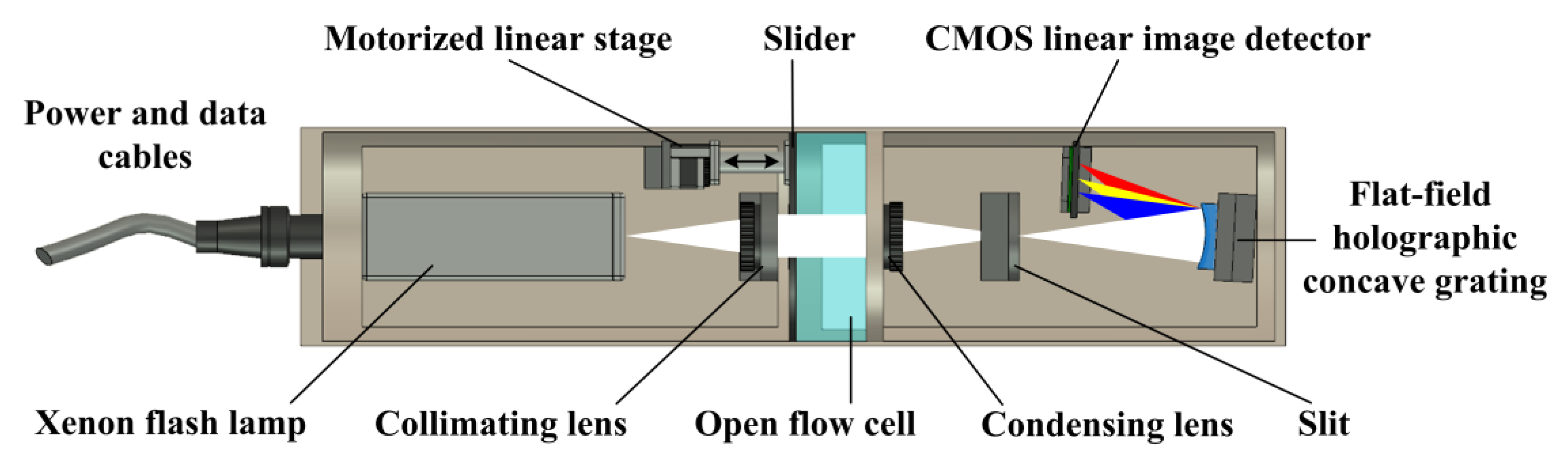
The structure of an UV-visible spectrometer probe with an adaptive optical path is shown in Figure 1. With compact design, it mainly comprises a xenon flash lamp, a collimating lens, a condensing lens, a slit, a flat-field holographic concave grating, a complementary metal oxide semiconductor (CMOS) linear image detector, a motorized linear stage and a slider. The xenon flash lamp light source, which delivers high stability and long service life, produces a broad spectral output from 185 nm to 2000 nm with a rated power of 5 W. The flat-field holographic concave grating works between 200 nm and 800 nm with reduced aberrations, bringing benefits of low light losses and simplified optical system. The CMOS linear image detector has 512 pixels, a spectral response range from 200 nm to 1000 nm, and on-chip charge amplifiers. During the operation of the UV-visible spectrometer probe, the light from the xenon flash lamp is collimated by the collimating lens and the beam passes through the water in the open flow cell. Then, the beam after absorption is condensed by the condensing lens and emitted from the slit. Finally, the flat-field holographic concave grating acts as a spectroscopic element and also an imaging element, while the CMOS linear image detector records the UV-visible absorption spectra. The UV-visible absorption spectra has an effective wavelength range from 200 nm to 800 nm and a resolution of 3 nm. Especially, the slider is driven by the motorized linear stage with a maximum speed of 10 mm/s, which makes the optical path in the open flow cell adjustable from 2 mm to 30 mm. The power and data cable, which supports power supply and data transmission, as well as the probe encapsulation are waterproof, so the whole probe can be placed in the water for in-situ analysis, the UV-visible absorption spectra can be acquired by a processor module for further process, and the optical path can be adaptive to internal and external information. As shown in Figure 2, the prototype of the UV-visible spectrometer probe is developed, which is used to analyze multiple parameters. Figure 2a shows the outside view of the prototype, Figure 2b shows the internal structure of the prototype, and Figure 2c shows the typical raw spectra of the blank and the multi-component mixture with TOC at 16 mg/L, nitrate nitrogen at 8 mg/L, nitrite nitrogen at 2 mg/L and turbidity at 20 NTU.
According to the Beer-Lambert law, the absorbance of a monochromatic beam which passes through a homogeneous medium is proportional to the product of the absorbing layer thickness and the absorbing component concentration [16,17]. For the absorbing component i and the wavelength λ, the absorbance Aλ,i can be written as:
where is the intensity of the incident radiation, is the intensity of the transmitted radiation, is a constant absorption coefficient at a given temperature for a specific medium, b is the absorbing layer thickness known as the adjustable optical path in the open flow cell here, and Ci is the absorbing component concentration. For a multi-component mixture tested by this UV-visible spectrometer probe, the total absorbance Aλ of the wavelength λ can be calculated as:
where and can derive from the UV-visible absorption spectra of a blank and the mixture respectively, n is the total number of absorbing components, λmin is the minimum wavelength which is 200 nm, and λmax is the maximum wavelength which is 800 nm. According to Equation (2), our UV-visible spectrometer probes can adjust the optical path b to tune the current absorbance curve at different pollutant concentrations, so that deviations from the Beer-Lambert law is reduced and accurate measurement in a wide dynamic range is feasible. Besides, the optical path adjustment is performed in the in-situ analysis mode and its granularity can be customized. The optical path adjusting rules and the quantitative multi-parameter analysis approach will be stated in Section 3.
2.2. Stationary and Mobile Wireless Sensor Nodes
In the sensing field of surface water, smart wireless sensor nodes are expected to complete sensing, storage, processing and communication in order to gather sufficient information of pollutant concentration distribution. Considering the complicated pollutant spreading conditions, not only stationary nodes but also mobile nodes are designed to localize the pollution source. By integration and miniaturization, buoys and USVs serve as stationary and mobile nodes respectively.
As shown in Figure 3, both stationary and mobile nodes are embedded with a processor module, a sensing module, a global positioning system (GPS) module, a general packet radio service (GPRS) module, and a power supply module. The processor module manages the resources of the other modules. The sensing module includes the UV-visible spectrometer probe, cameras and other sensors. The GPS module reports the current position of the node. The GPRS module supports wireless communication between nodes. The power supply module uses lithium batteries with auxiliary power supply from solar panels. In addition, each buoy is fixed by an anchor to prevent floating, while each USV is driven by double propellers with a maximum speed of 3 m/s and a cruise duration of 8 h. In the routine operation of wireless sensor nodes, the processor module acquires UV-visible absorption spectra and other raw data from the sensing module which are used to compute the local water quality multi-parameter measurements, and meanwhile obtains its own current position from the GPS module. Utilizing the GPRS module, the processor module share its information of water quality and node position with other nodes. Also, the processor module may send orders to adjust the optical path of the UV-visible spectrometer probe. For the USVs, there are four navigation modes, including remote control mode, fixed-path cruise mode, autonomous cruise mode and collaborative cruise mode. In the remote control mode, users can control the direction and speed with remote interfaces. In the fixed-path cruise mode, USVs move along predetermined navigation paths. In the autonomous cruise mode, USVs schedule their navigation paths automatically with local information. In the collaborative cruise mode, a group of USVs, usually accompanied by buoys, schedule their navigation paths collaboratively with shared information. USVs and buoys have opportunity to accomplish complicated tasks, such as water pollution source localization, in the collaborative cruise mode, which is mainly discussed in this paper.
2.3. Deployment for Water Quality Monitoring
In the water quality monitoring application, WSNs are composed of a number of wireless sensor nodes which are deployed in a two-dimensional sensing field and one sink node which is usually located on the shore. Reasonable deployment of wireless sensor nodes is required to guarantee the basic performance of WSNs.
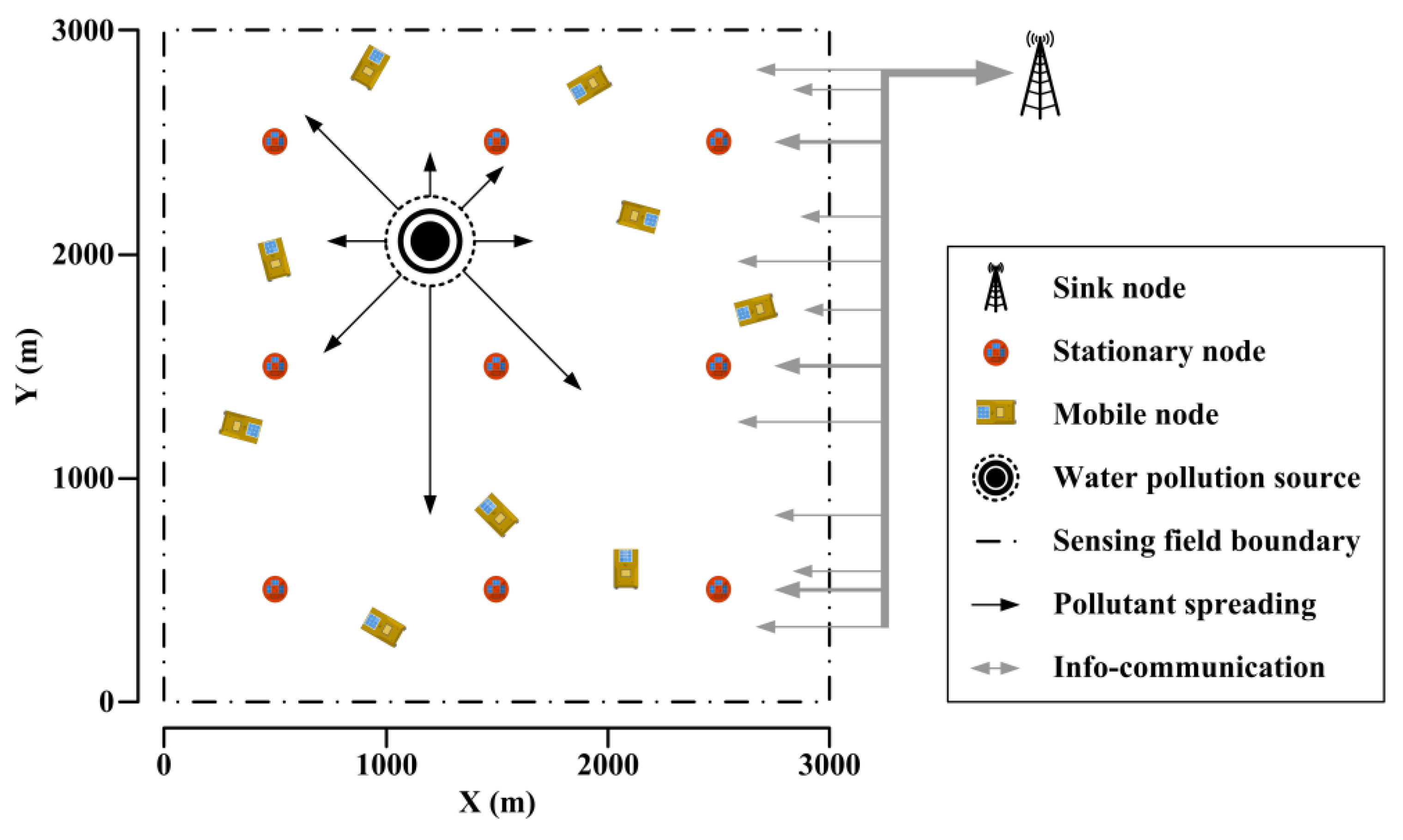
As shown in Figure 4, the stationary nodes are deployed regularly in fixed positions to provide stable and uniform coverage, while the mobile nodes are drifting with the waves in random positions to save energy. The sink node gathers local information from stationary nodes and mobile nodes after distributed processing, monitoring the water quality distribution in the sensing field. The task of water pollution source localization is triggered by events. For instance, when the spatial-temporal distribution of water quality satisfies pollution warning conditions or related commands are received from external systems, the water pollution source localization begins. Once a certain kind of pollution accident happens, pollutants spread from the water pollution source.
Since there are complicated pollutant spreading conditions, including pollutant concentration, wind direction, wind velocity, water flow direction, water flow velocity, etc., especially for large areas of water, it is difficult to build a precise pollutant spreading model from possible water pollution source to wireless sensor nodes in practical applications. Thus, the mobility of wireless sensor nodes is useful to localize the water pollution source. In order to find the water pollution source precisely and quickly, the sink node schedules paths of the mobile nodes based on the complete information of all the nodes. Therefore, the mobile nodes can move to proper positions and report detailed water quality distribution. The water pollution source localization method will be stated in Section 3. Because the sink node maintains a list of wireless sensor nodes to support their joining and leaving, the WSNs are robust and scalable.
3. Distributed Water Pollution Source Localization Method
With the defined WSNs, the problems of multi-parameter quantification, pollutant recognition, water pollution source searching and optical path adjustment can be formulated, and then the distributed Dual-PSO algorithm will be proposed to solve these problems and localize the water pollution source.
3.1. Problem Formulation
Each wireless sensor node has UV-visible absorption spectra and other raw data from the sensing module as well as its own current position from the GPS module. To localize the water pollution source in WSNs, there are four main problems, including multi-parameter quantification, pollutant recognition, water pollution source searching, and optical path adjustment.
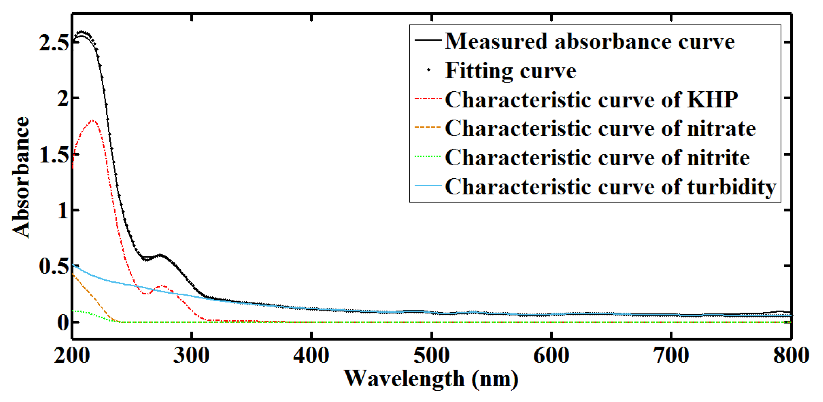
First of all, the local water quality multi-parameter measurements should be computed, using the UV-visible absorption spectra. As shown in Equation (2), the Beer-Lambert law is valid for mixtures of absorbing components fulfilling the condition that there are no interactions between these components. The relationship between absorbance curves and multiple parameters, such as TOC, nitrate nitrogen, turbidity, etc., should be investigated. Existing studies on water quality monitoring with UV-visible absorption spectra mostly concentrate on building analytical models for TOC or COD. For example, the regressive model between absorbance curves and TOC is built employing least squares support vector machine (LSSVM) [18]. It has been demonstrated that LSSVM has better performance than other approaches, such as principal component analysis (PCA) and partial least square (PLS). However, few efforts have been made to construct one synthesis analytical model of multiple parameters, considering the inherent features of continuous spectra. A scalable UV-visible spectral decomposition strategy is considered here, based on our former work on total-reflection X-ray fluorescence analysis [15]. As shown in Figure 5, the measured absorbance curve is decomposed into one background curve and a number of characteristic curves of possible components, which can be written as:
where F is the measured absorbance curve, f0 is the background curve, fi is the normalized characteristic curve of component i, and wi is the proportionality coefficient of component i. The background curve represents the contribution of uncontaminated water, which can be defined as the average absorbance during normal water quality monitoring, since the exogenous pollution accidents are mainly concerned. The normalized characteristic curves of multiple components, such as potassium hydrogen phthalate (KHP), nitrate, turbidity, etc., are shown in the figure, where KHP solution is prepared as a standard sample for TOC testing. According to Equation (2), the normalized characteristic curves can be stated as:
It can be found that the normalized characteristic curves do not depend on the adjustable optical path. These characteristic curves contains corresponding characteristic peaks, while water quality multi-parameter measurements can be derived from the proportionality coefficients. Hence, this problem becomes finding the optimal combination of proportionality coefficients to fit the measured absorbance curve. The objective function of combinatorial optimization problem can be formulated as:
By minimizing the objective function, the optimal set of proportionality coefficients can be found, where intelligent computing can be applied to solve the combinatorial optimization problem [19,20,21,22,23,24,25,26,27]. According to Equations (2)–(4), the water quality multi-parameter measurements can be calculated as:
The constant absorption coefficient Kλ,i can be determined by calibration, and the optical path b is known during testing. This strategy is suitable for multi-parameter quantification in various applications, because the characteristic curves of possible components can be added into the framework flexibly. Benefitting from optimal fitting in the whole spectral scope and the usage of inherent characteristic curves, it has potential to obtain high accuracy.
Then, the most sensitive parameter which reflects the water pollution source best should be recognized among the multiple parameters. In traditional water quality monitoring systems, the parameter of which the data exceed an established threshold is usually regarded as the most sensitive parameter. However, the establishment of threshold is based on experience, and it may lead to false positive alarms. The water quality distribution should be used to recognize the most sensitive parameter in order to avoid such problems. While the mobile nodes move to more positions in our case, more detailed water quality distribution can be obtained. Assuming that the number of stationary nodes and mobile nodes is s and m respectively, water quality multi-parameter measurements on the stationary nodes can be written as:
and those on the mobile nodes can be written as:
where x and y are X position and Y position of the wireless sensor nodes in the sensing field respectively, and l indicates the movement times of mobile nodes. The distribution of parameter i can be described as:
Thus, pattern recognition should be performed to distinguish a certain distribution from the others in order to find the most sensitive parameter.
Moreover, the mobility of wireless sensor nodes is used to search for the water pollution source. In this paper, it is assumed that the position of water pollution source is fixed, the pollutant concentration at this position is the highest, and the water quality distribution keep stable during searching. Since the sink node gathers the information of all the nodes, it can schedule paths of the mobile nodes utilizing the distribution of the most sensitive parameter. Hence, it becomes an extremum seeking problem in the sensing field. Also, intelligent computing can be considered to solve this problem.
In addition, the sensing object of wireless sensor nodes varies from high-quality surface water to heavily polluted water, so the optical path of each wireless sensor node should be properly adjusted to achieve reliable sensing. According to Equation (2), the absorbance curve can be tuned at different pollutant concentrations with customized granularity. Assuming that the optical path can be adjusted exponentially, it can be written as:
where b0 is the default optical path, ϕ is the scaling unit, d is the scaling coefficient which is an integer, bmin is the minimum optical path which is 2 mm, and bmax is the maximum optical path which is 30 mm. Commonly, the same absorption coefficient Kλ,i can be simply used when the optical path is adjusted, so Equation (2) can be stated as:
where:
Therefore, the absorbance curve of the adjusted optical path can be predicted with Equation (11), which can be utilized to set the optical path adjusting rules.
3.2. Dual-PSO Algorithm
Considering the mentioned requirements of water pollution source localization and the capacities of WSNs, a distributed algorithm is developed here. For the problems of multi-parameter quantification and water pollution source searching, similar intelligent computing approaches are considered. Some algorithms, such as steepest descent and genetic algorithms (GA), may be discussed in optimization problems [28]. It has been shown that GA has better performance than steepest descent. In our case, however, the mobile nodes act as natural particles in water pollution source searching, different solution dimensions of proportionality coefficients require different granularity in multi-parameter quantification, and the whole procedure needs to be quick and low cost, where particle swarm optimization (PSO) is preferred. Kennedy et al., developed PSO in 1995 based on the analogy of swarms of birds and fish schools [29,30]. PSO is an efficient optimization tool for solving combinatorial optimization problems and dynamic optimization problems. Like other evolutionary algorithms, PSO uses fitness as criterion to evolve the behavior of the solution population. Potential solutions, namely particles, fly through the searching space. Each particle keeps track of the best position it has achieved so far, which represents a particle experiment. Another kind of experiment is the best position which has been achieved by any companion of the particle so far. The particle velocity is constantly adjusted according to the two kinds of experiences. The diagram of the Dual-PSO algorithm is shown in Figure 6, where one PSO procedure computes the water quality multi-parameter measurements on each wireless sensor node and the other one searches for the water pollution source with real particles. With distributed processing, only a small amount of necessary information, such as multi-parameter measurements and position coordinates, is exchanged between nodes, otherwise centralized processing demands more communication cost for raw data transmission. Meanwhile, the entropy of water quality multi-parameter distribution which reflects the disorder degree is introduced as a metric to dynamically recognize the most sensitive parameter during searching, because it has low computational complexity and does not need high resolution input [31,32,33]. Besides, the optical path adjusting rules are set to work in a proper absorbance range adaptively for each wireless sensor node so that reliable sensing at different pollutant concentrations is guaranteed. The pseudo-code for the Dual-PSO algorithm is outlined in Algorithm 1, where more water quality parameters from UV-visible spectrometer probes or other sensors, more wireless sensor nodes and larger sensing fields can be easily extended.
| Algorithm 1: Dual-PSO |
| One PSO procedure is performed globally to search for the water pollution source on the sink node and wireless sensor nodes. It is assumed that there are M wireless sensor nodes, of which s are stationary nodes and m are mobile nodes. For represents the current position of wireless sensor node α: The maximum iteration of global PSO is set as . For For The absorbance level on wireless sensor node α is defined as: Assuming the current optical path is: With the adjusted optical path , the absorbance curve is updated. The other PSO procedure is performed locally to compute water quality multi-parameter measurements on wireless sensor node and the population of particles is set as N. For represents the current solution, initialized randomly in the solution space: The maximum iteration of local PSO is set as . For The global best solution is defined as: The weighted particle velocity is updated as: The solution of each particle is updated as: End The optimization result of the proportionality coefficients is recorded as: A discrete function of water quality multi-parameter distribution is maintained as: The entropy of water quality multi-parameter distribution is evaluated. For The discrete distribution function of parameter i is given. Measurements in its range are sorted in ascending order as: The entropies are compared, and parameter γ with the minimum entropy is recognized as the most sensitive parameter of the water pollution source. The global best position is defined as: The weighted velocity is updated as: The new position of each wireless sensor node is scheduled as: End The optimization result of the water pollution source position is recorded. |
4. Results and Discussion
A simulation scene is constructed as shown in Figure 4. The sensing field is 3000 m long and 3000 m wide, where nine stationary nodes are deployed regularly in fixed positions and nine mobile nodes are drifting with the waves in random initial positions. During water pollution source localization, the sink node gathers multi-parameter measurements and position coordinates from all wireless sensor nodes, and sends the scheduled paths to the mobile nodes. For the designed UV-visible spectrometer probes, multiple parameters, including TOC, nitrate nitrogen, nitrite nitrogen and turbidity, are considered. In the optical path adjusting rules, the default optical path b0 is set as 10 mm, the scaling unit ϕ is set as 2, the minimum absorbance level is set as 0.3, and the maximum absorbance level is set as 0.7.
The efficiency of multi-parameter quantification is examined first. KHP solution is prepared as a standard sample for TOC testing, potassium nitrate solution is prepared as a standard sample for nitrate nitrogen testing, sodium nitrite solution is prepared as a standard sample for nitrite nitrogen testing, and formazine solution is prepared as a standard sample for turbidity testing. Both single-parameter samples and multi-parameter samples are used in the experiments. As shown in Figure 7, normalized characteristic curves of multiple parameters are acquired. For a measured absorbance curve, quantification with Dual-PSO is accomplished on a single wireless sensor node. A multi-parameter sample with TOC at 16 mg/L, nitrate nitrogen at 8 mg/L, nitrite nitrogen at 2 mg/L and turbidity at 20 NTU is tested. Figure 8 shows the measured absorbance curve, the fitting curve and the multi-parameter contributions. It can be found that the measured absorbance curve is approximated with high accuracy. More multi-parameter samples are tested to examine the performance utilizing adaptive optical path. Table 1 gives the relative error (RE) and the relative standard deviation (RSD) of TOC, nitrate nitrogen (NO3-N) and turbidity measurements, compared with the LSSVM method. The optical path (OP) switches between 5 mm, 10 mm and 20 mm in our method, while it keeps 10 mm in LSSVM. It is shown that the quantification performance is enhanced by our method, especially in the case that there is opportunity to optimize the optical path. With the designed UV-visible spectrometer probe and the Dual-PSO algorithm, optimal fitting in the whole spectral scope is taken into account and deviations from the Beer-Lambert law are reduced, so RE and RSD are smaller and do not vary drastically when the pollutant concentrations vary in a wide range. Besides, simultaneous and fast quantification of multiple parameters is achieved without the requirement of a large number of training populations.
In the sensing field, the water quality multi-parameter distribution is simulated as shown in Figure 9. Quantitative analysis of TOC, nitrate nitrogen and turbidity are considered, and TOC is set as the most sensitive parameter which reflects the water pollution source best. The Dual-PSO algorithm is performed on the wireless sensor nodes and the sink node to identify and localize the water pollution source. The entropy of water quality multi-parameter distribution during searching is calculated dynamically as shown in Figure 10. It can be found that the entropy of TOC distribution keeps lower than that of nitrate nitrogen or turbidity distribution, and the difference becomes more significant with more detailed distribution during searching. Thus, the entropy is an effective metric to recognize the most sensitive parameter, of which the disorder degree is lower than that of the other parameters which are more evenly distributed. In this way, more parameters from the UV-visible spectrometer probe or other sensors can be easily added into the Dual-PSO algorithm for recognition.
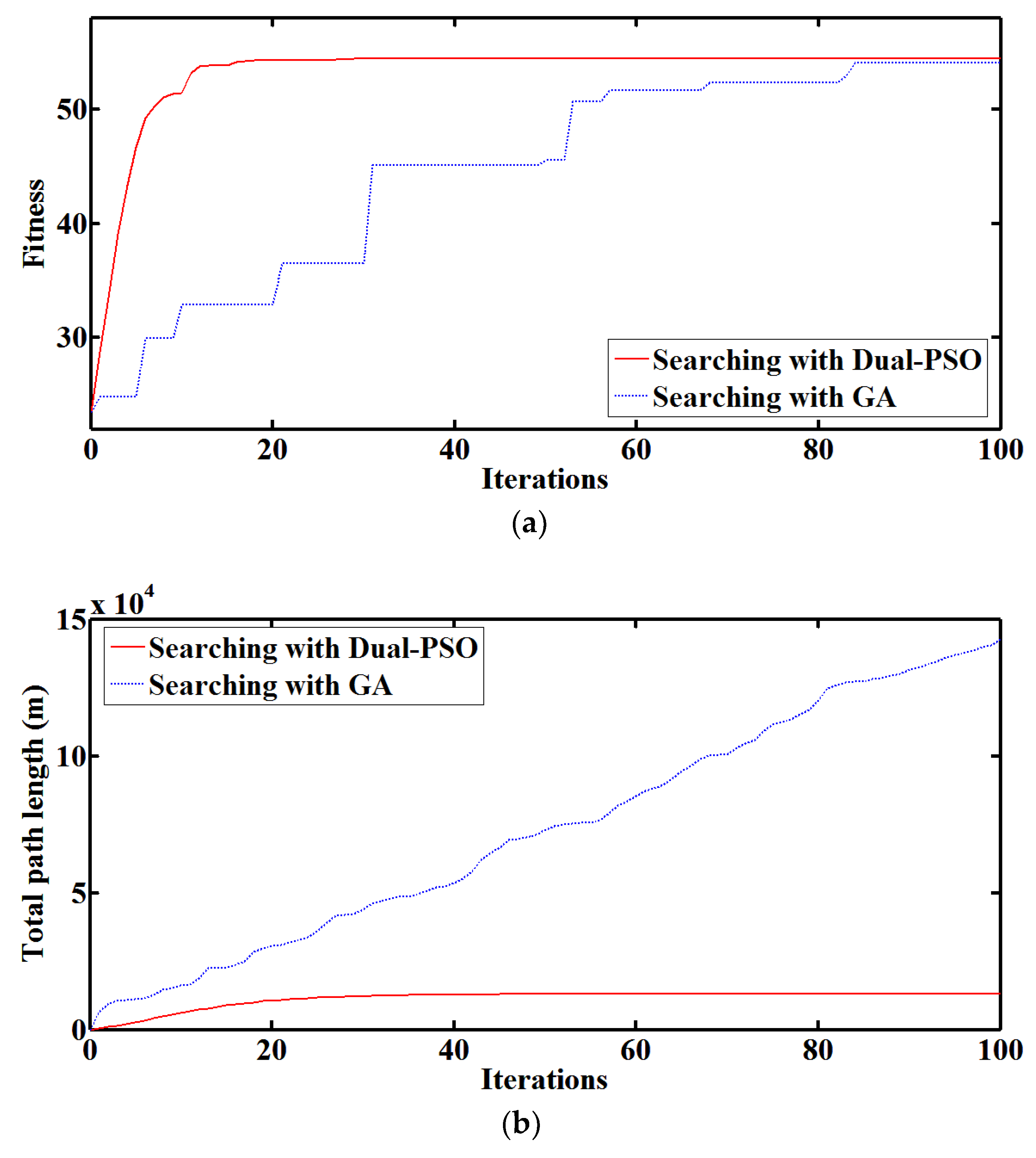
In Figure 11, water pollution source searching with Dual-PSO and GA is compared, where GA uses the same swarm of mobile nodes as Dual-PSO. It can be seen that the convergence of Dual-PSO is faster than that of GA and the total path length of mobile nodes in Dual-PSO is much shorter than that in GA. Dual-PSO finished searching within 20 iterations, while GA does not achieve the same searching result after even 80 iterations.
The Dual-PSO algorithm enjoys high convergence speed and global optimization ability. In Dual-PSO, the scheduled path of each mobile nodes is smoother, the path length of each mobile node within one single iteration decreases during searching, and the path lengths of different mobile nodes are balanced. That is because PSO is based on the analogy of swarms of birds and fish schools. Given the maximum speed of mobile nodes, each iteration can be completed within 1 minute in Dual-PSO, while the time consumption of each single iteration is unpredictable and the longest iteration in this case lasts over 5 min in GA. Moreover, the step length of searching can be adaptive to different mobile abilities or deployment densities in Dual-PSO. Therefore, efficient water pollution source localization can be achieved by the Dual-PSO algorithm with less time consumption, less power consumption and more feasible navigation paths. Also, it can be realized that water quality measurements, no matter direct measurements or indirect measurements, which reflect the pollutant concentration distribution is applicable for searching, which means that there is opportunity to miniaturize and strengthen the wireless sensor nodes with more optional sensors and soft measurement models. During water pollution source localization, the water quality multi-parameter distribution is simulated under complicated pollutant spreading conditions, and the proposed method can find the water pollution source within 20 min. When pollutant concentrations vary in a wide range, the UV-visible spectrometer probes keep acceptable sensing performance. The Dual-PSO algorithm obtains better multi-parameter quantification results than LSSVM and also obtains better water pollution source searching results than GA. Besides, the most sensitive parameter is efficiently recognized using the entropy of water quality multi-parameter distribution during localization.
5. Conclusions
To identify and localize water pollution sources efficiently in surface water-facing pollution accidents, this paper proposes a distributed water pollution source localization method in WSNs. Firstly, WSNs are established for water quality monitoring, where wireless sensor nodes equipped with well-designed UV-visible spectrometer probes are deployed to analyze multiple parameters. Buoys and USVs serve as stationary and mobile nodes respectively, and the optical path of each UV-visible spectrometer probe is adjustable. Then, the Dual-PSO algorithm is presented to solve the problems of multi-parameter quantification, pollutant recognition, water pollution source searching and optical path adjustment. One PSO procedure computes the water quality multi-parameter measurements on each wireless sensor node and the other one searches for the water pollution source with real particles. With distributed processing, only a small amount of necessary information, including multi-parameter measurements, position coordinates and scheduled paths, is exchanged between nodes. The entropy of water quality multi-parameter distribution which reflects the disorder degree is introduced as a metric to dynamically recognize the most sensitive parameter during searching. The optical path adjusting rules are set so that each wireless sensor node can work in a proper absorbance range adaptively for reliable sensing. Finally, experiments and simulations demonstrate the efficiency of quantitative multi-parameter analysis and water pollution source localization. The Dual-PSO algorithm enhances the multi-parameter quantification performance without the requirement of a large number of training populations, and it completes the pollution source searching with less time consumption, less power consumption and more feasible navigation paths. The main contribution of this paper is that the total solution of WSNs is investigated to identify and localize water pollution sources efficiently under complicated pollutant spreading conditions, the novel distributed Dual-PSO algorithm is studied particularly to solve the related problems, the adaptive optical path mechanism reduces deviations from the Beer-Lambert law in a wide measurement range, and the scalable framework is constructed to support the extension of more water quality parameters from UV-visible spectrometer probes or other sensors, more wireless sensor nodes and larger sensing fields. This paper focuses on the application scenario of one certain stationary water pollution source, making use of multiple parameters from UV-visible spectrometer probes. In future research, the distributed water pollution source localization method shall be evolved, considering more application scenarios, such as multiple water pollution sources with different pollutants, mobile water pollution sources, interactions between multi-components, extension of parameters, and energy-aware management of mobile nodes.
Acknowledgments
This work is supported by the National Key Scientific Instrument and Equipment Development Project of China No. 2012YQ060115.
Author Contributions
Junjie Ma designed the adaptive optical path mechanism, developed the Dual-PSO algorithm, conducted the experiments and simulations, and provided the manuscript. Fansheng Meng, Yuexi Zhou and Yeyao Wang helped to design the scheme and the algorithm. Ping Shi helped to establish the basic UV-visible spectrometer system and helped to carry out the experiments. All authors were involved with the revisions of the manuscript.
Conflicts of Interest
The authors declare no conflict of interest.
References
- Gholizadeh, M.H.; Melesse, A.M.; Reddi, L. Water quality assessment and apportionment of pollution sources using APCS-MLR and PMF receptor modeling techniques in three major rivers of South Florida. Sci. Total Environ. 2016, 566, 1552–1567. [Google Scholar] [CrossRef] [PubMed]
- Zhao, Y.; Xia, X.H.; Yang, Z.F. Assessment of water quality in Baiyangdian Lake using multivariate statistical techniques. Procedia Environ. Sci. 2012, 13, 1213–1226. [Google Scholar] [CrossRef]
- Kim, C.; Eom, J.B.; Jung, S.; Ji, T. Detection of organic compounds in water by an optical absorbance method. Sensors 2016, 16, 61. [Google Scholar] [CrossRef] [PubMed]
- Xu, L.; Luo, Y. A new technology for water quality monitoring based on UV-visible spectrum analysis. Spectrosc. Spectr. Anal. 2014, 34, 443–444. [Google Scholar]
- Cao, H.; Qu, W.; Yang, X.; Jia, S.; Wang, C.; Lu, C. Research on rapid determination of organic matter concentration in aquaculture water based on UV-visible spectroscopy. Spectrosc. Spectr. Anal. 2014, 34, 3015–3019. [Google Scholar]
- Kus, M.; Ribbens, S.; Meynen, V.; Cool, P. Microvolume TOC analysis as useful tool in the evaluation of lab scale photocatalytic processes. Catalysts 2013, 3, 74–87. [Google Scholar] [CrossRef]
- Zhao, Y.; Li, Y.; Zhen, Y.; Fang, Y. A novel monitoring system for COD using optical ultraviolet absorption method. Procedia Environ. Sci. 2011, 10, 2348–2353. [Google Scholar]
- Tang, B.; Zhao, J.; Wei, B.; Jiang, S.; Luo, J. A method of optimizing the prediction model for the determination of water COD by using UV-visible spectroscopy. China Environ. Sci. 2015, 35, 478–483. [Google Scholar]
- Tang, B.; Wei, B.; Wu, D.; Mi, D.; Zhao, J.; Feng, P.; Jiang, S.; Mao, B. Experimental research of turbidity influence on water quality monitoring of COD in UV-visible spectroscopy. Spectrosc. Spectr. Anal. 2014, 34, 3020–3024. [Google Scholar]
- Wu, D.; Wei, B.; Feng, P.; Tang, B.; Liu, J. Denoising algorithm of UV-visible spectroscopy on water quality detection based on two-dimension restructuring and dynamic pane. Spectrosc. Spectr. Anal. 2016, 36, 1044–1050. [Google Scholar]
- Tang, B.; Wei, B.; Mao, B.; Zhao, J.; Feng, P. Noise analysis and denoising research on the UV-visible absorption spectroscopy water quality detection system. Laser Optoelectron. Prog. 2014, 51, 197–203. [Google Scholar] [CrossRef]
- Tang, G.; Wei, B.; Wu, D.; Feng, P.; He, P.; Liu, J.; Chen, M. Research on compression and reconstruction algorithm of spectral data in water quality monitoring. Environ. Sci. Technol. 2016, 39, 6–10. [Google Scholar]
- Wang, X.; Ma, J.; Wang, S.; Bi, D. Cluster-based dynamic energy management for collaborative target tracking in wireless sensor networks. Sensors 2007, 7, 1193–1215. [Google Scholar] [CrossRef]
- Wang, X.; Ma, J.; Wang, S. Parallel energy-efficient coverage optimization with maximum entropy clustering in wireless sensor networks. J. Parallel Distrib. Comput. 2009, 69, 838–847. [Google Scholar] [CrossRef]
- Ma, J.; Wang, Y.; Yang, Q.; Liu, Y.; Shi, P. Intelligent simultaneous quantitative online analysis of environmental trace heavy metals with total-reflection X-ray fluorescence. Sensors 2015, 15, 10650–10675. [Google Scholar] [CrossRef] [PubMed]
- Hou, D.; Zhang, J.; Chen, L.; Huang, P.; Zhang, G. Water quality analysis by UV-visible spectroscopy: A review of methodology and application. Spectrosc. Spectr. Anal. 2013, 33, 1839–1844. [Google Scholar]
- Zhao, Y.; Li, Y.; Guo, Y.; Gu, B.; Yang, Z. A novel technology for water quality testing based on UV spectral analysis. Spectrosc. Spectr. Anal. 2012, 32, 1301–1305. [Google Scholar]
- Liu, X.; Zhang, H. Rapid determination of COD in aquaculture water based on LSSVM with UV-visible spectroscopy. Spectrosc. Spectr. Anal. 2014, 34, 2804–2807. [Google Scholar]
- Wang, X.; Wang, S.; Ma, J. An improved particle filter for target tracking in sensor systems. Sensors 2007, 7, 144–156. [Google Scholar] [CrossRef]
- Wang, X.; Ma, J.; Ding, L.; Bi, D. Robust forecasting for energy efficiency of wireless multimedia sensor networks. Sensors 2007, 7, 2779–2807. [Google Scholar] [CrossRef] [PubMed]
- Wang, X.; Ma, J.; Wang, S.; Bi, D. Time series forecasting energy-efficient organization of wireless sensor networks. Sensors 2007, 7, 1766–1792. [Google Scholar] [CrossRef] [PubMed]
- Taormina, R.; Chau, K.W.; Sivakumar, B. Neural network river forecasting through baseflow separation and binary-coded swarm optimization. J. Hydrol. 2015, 529, 1788–1797. [Google Scholar] [CrossRef]
- Gholami, V.; Chau, K.W.; Fadaee, F.; Torkaman, J.; Ghaffari, A. Modeling of groundwater level fluctuations using dendrochronology in alluvial aquifers. J. Hydrol. 2015, 529, 1060–1069. [Google Scholar] [CrossRef]
- Wang, W.C.; Xu, D.M.; Chau, K.W.; Chen, S. Improved annual rainfall-runoff forecasting using PSO–SVM model based on EEMD. J. Hydroinform. 2013, 15, 1377–1390. [Google Scholar] [CrossRef]
- Zhang, S.; Chau, K.W. Dimension reduction using semi-supervised locally linear embedding for plant leaf classification. In Emerging Intelligent Computing Technology and Applications; Springer: Berlin/Heidelberg, Germany, 2009; pp. 948–955. [Google Scholar]
- Wu, C.L.; Chau, K.W.; Fan, C. Prediction of rainfall time series using modular artificial neural networks coupled with data-preprocessing techniques. J. Hydrol. 2010, 389, 146–167. [Google Scholar] [CrossRef]
- Chau, K.W.; Wu, C.L. A hybrid model coupled with singular spectrum analysis for daily rainfall prediction. J. Hydroinform. 2010, 12, 458–473. [Google Scholar] [CrossRef]
- Ma, J.; Wang, Y.; Yang, Q.; Liu, Y.; Shi, P. Intelligent simultaneous quantification of environmental trace elements with total reflection X-ray fluorescence. In Proceedings of the IEEE 15th International Conference on Environment and Electrical Engineering, Rome, Italy, 10–13 June 2015; pp. 1580–1586. [Google Scholar]
- Wang, X.; Ma, J.; Wang, S.; Bi, D. Distributed particle swarm optimization and simulated annealing for energy-efficient coverage in wireless sensor networks. Sensors 2007, 7, 628–648. [Google Scholar] [CrossRef]
- Wang, X.; Ma, J.; Wang, S. Distributed energy optimization for target tracking in wireless sensor networks. IEEE Trans. Mobile Comput. 2009, 9, 73–86. [Google Scholar] [CrossRef]
- Wang, C.; Wu, F.; Zhao, H.; Lu, S. Temporal information entropy and its application in the detection of spatio-temporal changes in vegetation coverage based on remote sensing images. Acta Ecol. Sin. 2017, 37, 7359–7367. [Google Scholar]
- Al-Omari, A.I. Estimation of entropy using random sampling. J. Comput. Appl. Math. 2014, 261, 95–102. [Google Scholar] [CrossRef]
- Yentes, J.M.; Hunt, N.; Schmid, K.K. The appropriate use of approximate entropy and sample entropy with short data sets. Ann. Biomed. Eng. 2013, 41, 349–365. [Google Scholar] [CrossRef] [PubMed]
Figure 1.
The structure of the UV-visible spectrometer probe with adaptive optical path.

Figure 2.
The prototype of the UV-visible spectrometer probe: (a) The outside view; (b) The internal structure; (c) The typical raw spectra of the blank and the multi-component mixture.
Figure 2.
The prototype of the UV-visible spectrometer probe: (a) The outside view; (b) The internal structure; (c) The typical raw spectra of the blank and the multi-component mixture.
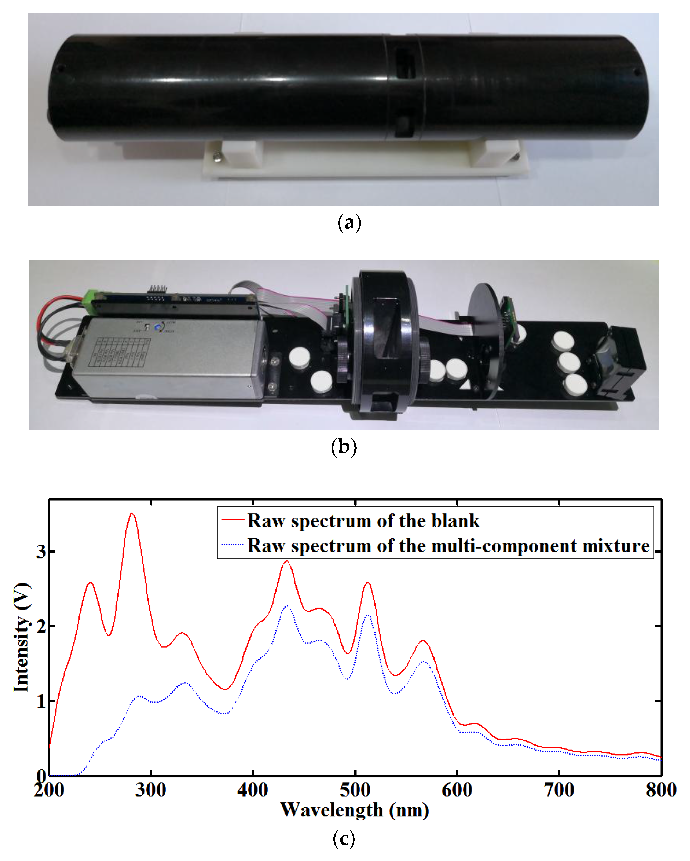
Figure 3.
Configuration of stationary and mobile wireless sensor nodes.
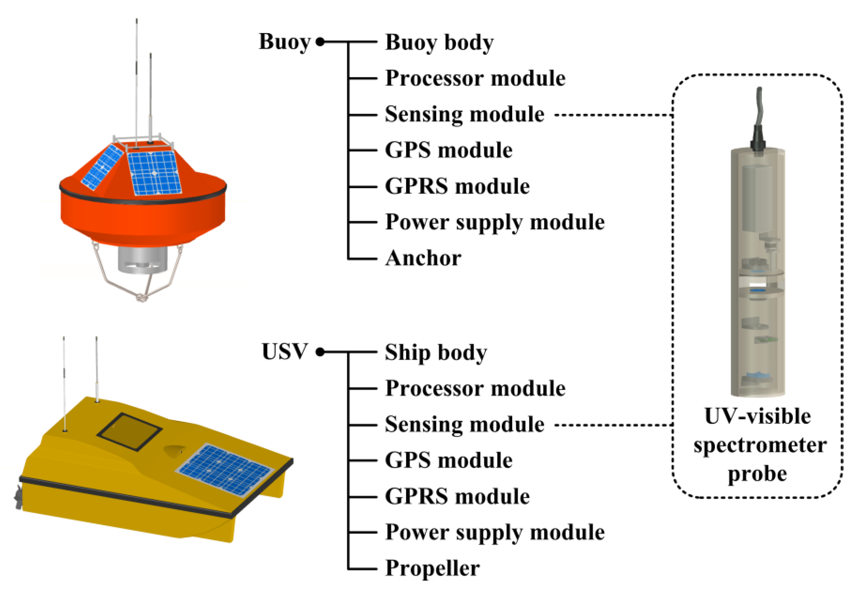
Figure 4.
The WSN deployment for water quality monitoring.

Figure 5.
The decomposition strategy of the measured absorbance curve.
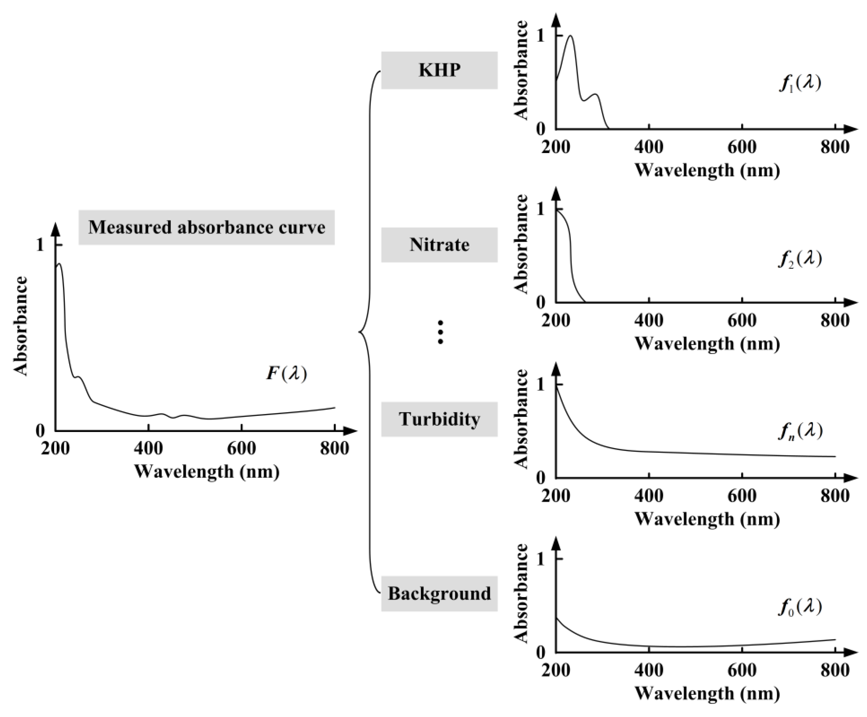
Figure 6.
The diagram of the Dual-PSO algorithm.
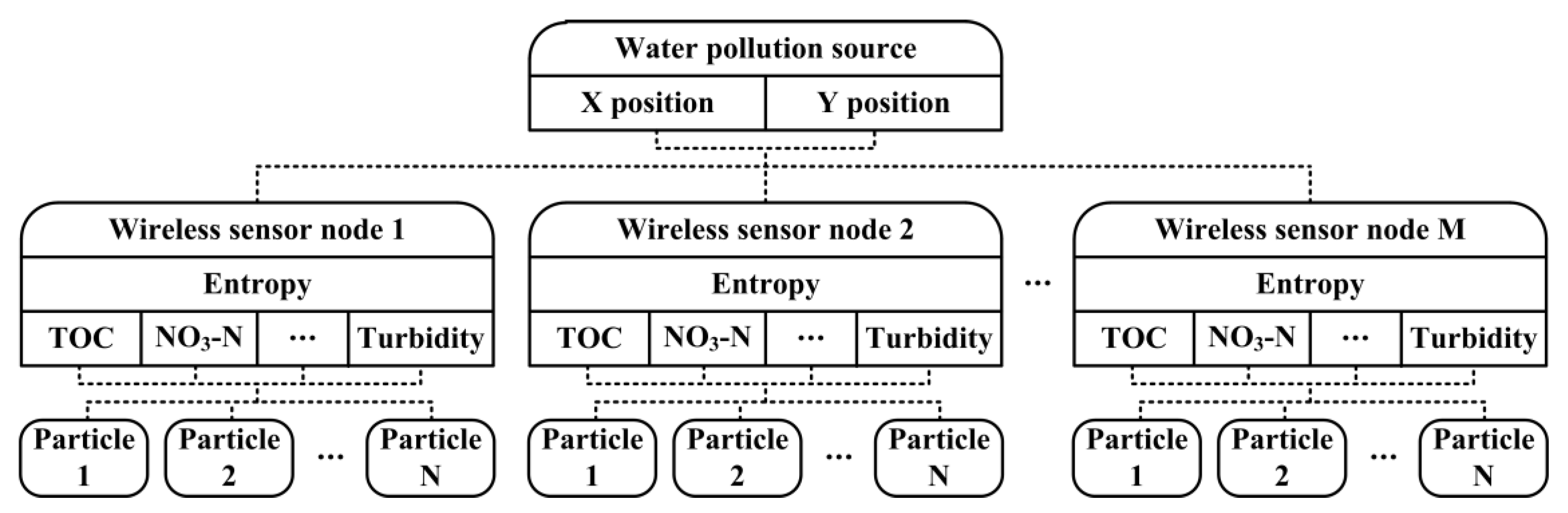
Figure 7.
Normalized characteristic curves of multiple parameters.
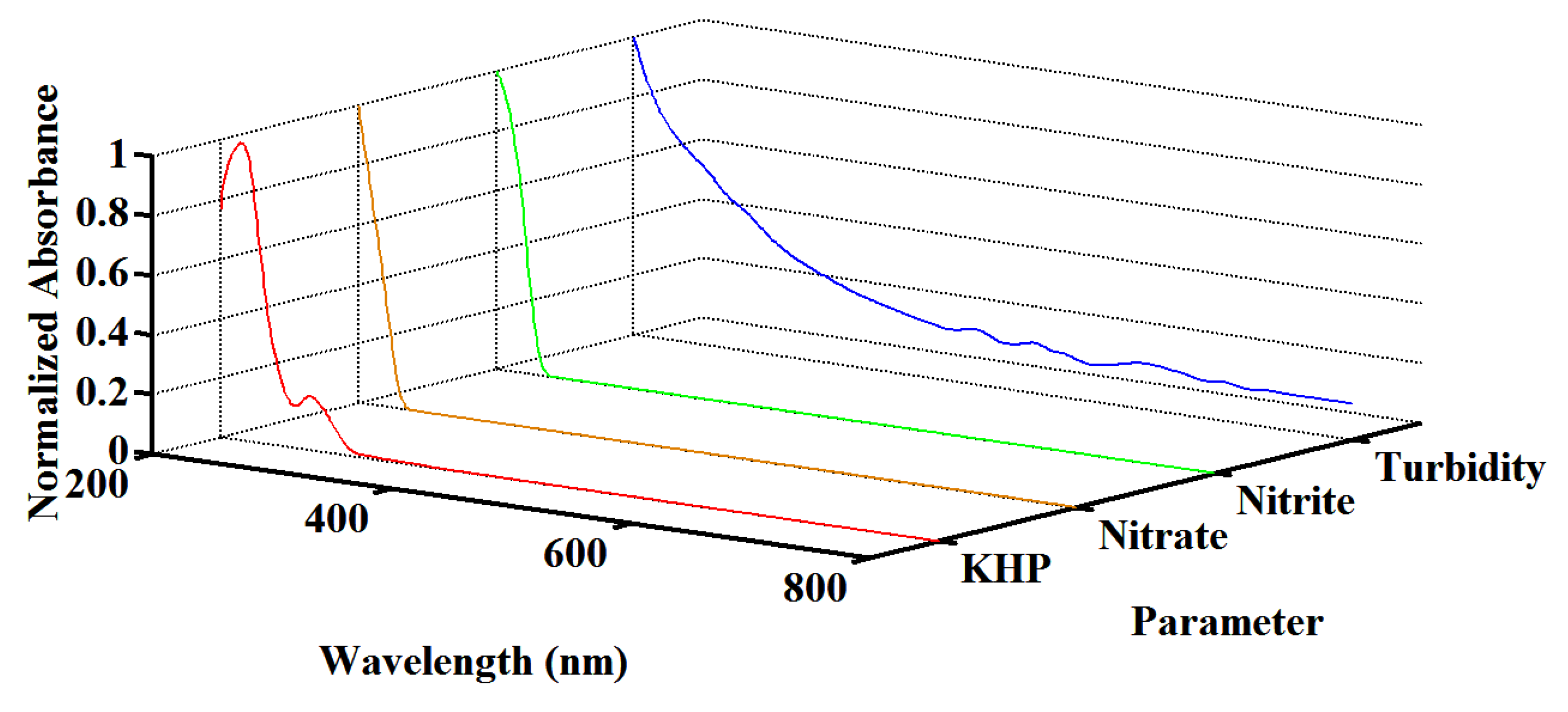
Figure 8.
The fitting curve of measured absorbance curve in multi-parameter quantification.

Figure 9.
The simulated water quality multi-parameter distribution.
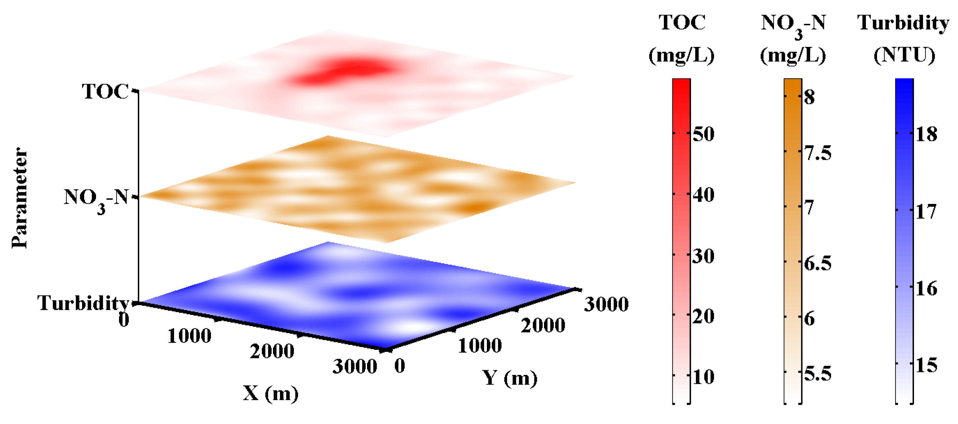
Figure 10.
The entropy of water quality multi-parameter distribution during searching.
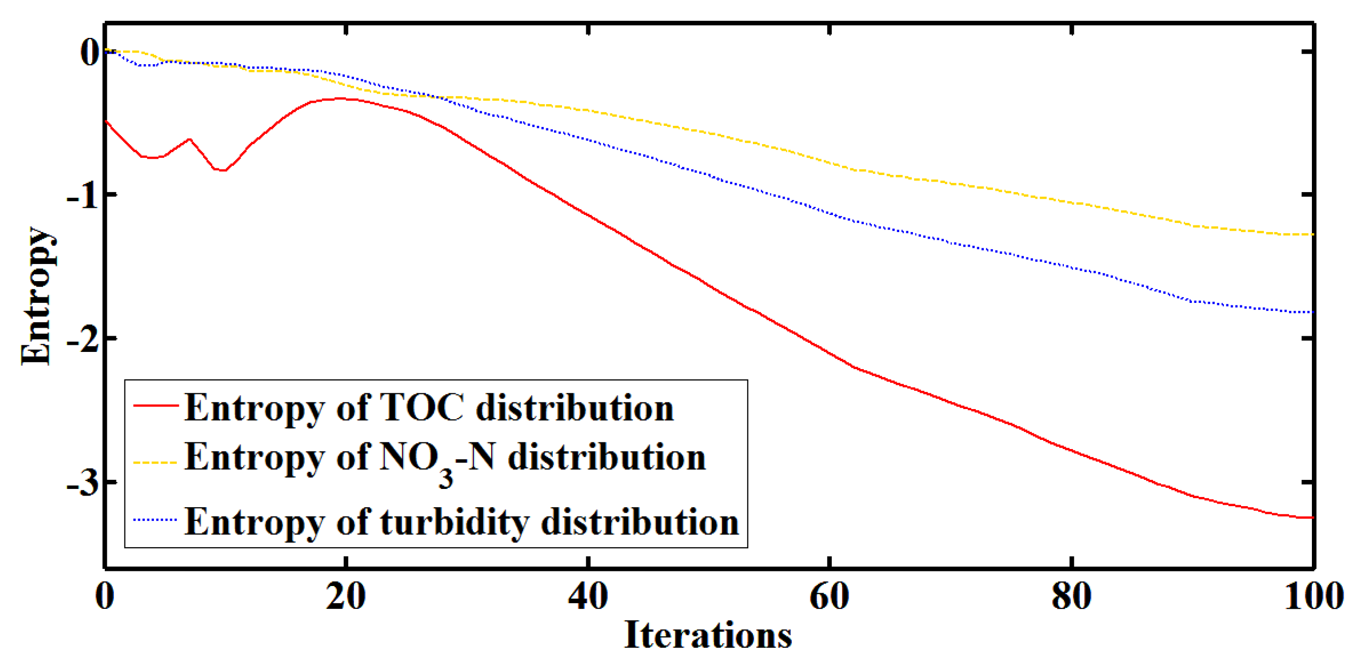
Figure 11.
Comparison of water pollution source searching with Dual-PSO and GA: (a) The convergence curves; (b) The total path length of mobile nodes during searching.
Figure 11.
Comparison of water pollution source searching with Dual-PSO and GA: (a) The convergence curves; (b) The total path length of mobile nodes during searching.


Table 1.
Comparison of multi-parameter quantification with Dual-PSO and LSSVM.
| Sample No. | Parameter | Concentration | Dual-PSO | LSSVM | ||||
|---|---|---|---|---|---|---|---|---|
| OP | RE | RSD | OP | RE | RSD | |||
| 1 | TOC | 8 mg/L | 20 mm | −4.23% | 1.03% | 10 mm | −6.97% | 2.36% |
| NO3-N | 4 mg/L | 4.85% | 1.49% | 6.13% | 3.10% | |||
| Turbidity | 10 NTU | 3.06% | 2.05% | 5.50% | 3.89% | |||
| 2 | TOC | 16 mg/L | 10 mm | −3.52% | 1.12% | −4.16% | 1.25% | |
| NO3-N | 8 mg/L | 4.59% | 1.47% | 5.73% | 1.62% | |||
| Turbidity | 20 NTU | 2.70% | 2.08% | 2.82% | 2.19% | |||
| 3 | TOC | 32 mg/L | 5 mm | −7.36% | 1.26% | −12.55% | 2.85% | |
| NO3-N | 16 mg/L | 5.02% | 1.51% | 15.13% | 2.93% | |||
| Turbidity | 40 NTU | 3.92% | 2.16% | 6.12% | 3.67% | |||
© 2018 by the authors. Licensee MDPI, Basel, Switzerland. This article is an open access article distributed under the terms and conditions of the Creative Commons Attribution (CC BY) license (http://creativecommons.org/licenses/by/4.0/).
Share and Cite
MDPI and ACS Style
Ma, J.; Meng, F.; Zhou, Y.; Wang, Y.; Shi, P. Distributed Water Pollution Source Localization with Mobile UV-Visible Spectrometer Probes in Wireless Sensor Networks. Sensors 2018, 18, 606. https://doi.org/10.3390/s18020606
AMA Style
Ma J, Meng F, Zhou Y, Wang Y, Shi P. Distributed Water Pollution Source Localization with Mobile UV-Visible Spectrometer Probes in Wireless Sensor Networks. Sensors. 2018; 18(2):606. https://doi.org/10.3390/s18020606
Chicago/Turabian StyleMa, Junjie, Fansheng Meng, Yuexi Zhou, Yeyao Wang, and Ping Shi. 2018. "Distributed Water Pollution Source Localization with Mobile UV-Visible Spectrometer Probes in Wireless Sensor Networks" Sensors 18, no. 2: 606. https://doi.org/10.3390/s18020606
Note that from the first issue of 2016, this journal uses article numbers instead of page numbers. See further details here.