Event-Triggered Fault Estimation for Stochastic Systems over Multi-Hop Relay Networks with Randomly Occurring Sensor Nonlinearities and Packet Dropouts

Key Laboratory of Advanced Process Control for Light Industry (Ministry of Education), Jiangnan University, Wuxi 214122, China
*
Author to whom correspondence should be addressed.
Sensors 2018, 18(3), 731; https://doi.org/10.3390/s18030731
Submission received: 29 January 2018
/
Revised: 24 February 2018
/
Accepted: 26 February 2018
/
Published: 28 February 2018
(This article belongs to the Special Issue Sensors for Fault Detection)
Abstract
:Wireless sensors have many new applications where remote estimation is essential. Considering that a remote estimator is located far away from the process and the wireless transmission distance of sensor nodes is limited, sensor nodes always forward data packets to the remote estimator through a series of relays over a multi-hop link. In this paper, we consider a network with sensor nodes and relay nodes where the relay nodes can forward the estimated values to the remote estimator. An event-triggered remote estimator of state and fault with the corresponding data-forwarding scheme is investigated for stochastic systems subject to both randomly occurring nonlinearity and randomly occurring packet dropouts governed by Bernoulli-distributed sequences to achieve a trade-off between estimation accuracy and energy consumption. Recursive Riccati-like matrix equations are established to calculate the estimator gain to minimize an upper bound of the estimator error covariance. Subsequently, a sufficient condition and data-forwarding scheme are presented under which the error covariance is mean-square bounded in the multi-hop links with random packet dropouts. Furthermore, implementation issues of the theoretical results are discussed where a new data-forwarding communication protocol is designed. Finally, the effectiveness of the proposed algorithms and communication protocol are extensively evaluated using an experimental platform that was established for performance evaluation with a sensor and two relay nodes.
1. Introduction
The increased use of battery-powered wireless sensors can improve productivity and reduce installation costs in industrial processes. A variety of battery-powered wireless sensors span a wide range of applications including area detection, environmental sensing, industrial monitoring and control, etc. [1]. In these applications, data packet loss is often encountered in various practical environments owing to bandwidth constraints; and then, wireless sensors are practically often made under harsh environments including both uncontrollable elements and aggressive conditions [2]. In this case, estimator or observer results [3,4] based on the linear sensor may not provide a reliable solution and are not applicable. It should be pointed out that the size and costs of sensor nodes may result in constraints on resources such as energy, memory and computation speeds [5,6,7,8]. Such constraints may lead to development of new estimators and data transmission schemes against these constraints we mentioned above. On the other hand, it is also recognized that the failures of components appear always in many practical engineering systems. The occurrence of faults in sensors, actuator or process (plant) failures may drastically modify the system behavior, resulting in performance degradation or even instability. For the purpose of increasing the safety and reliability of networked controlled systems, fault diagnosis research and their applications to a wide range of industrial and commercial processes have been the subjects of intensive investigations over the past two decades [9,10,11,12]. Many fruitful results for a variety of systems have been reported [13,14,15,16,17,18,19,20,21].
In the past few years, a number of results related to state and/or fault estimation for a variety of systems with packet dropouts and/or sensor nonlinearities have been established in terms of all sorts of methods. Some examples are mentioned here. Linear and nonlinear estimation problems were tackled for missing measurements in [22], where the nonlinear function of sensor was modeled as a sector-bound condition. A robust filter was designed in [23] against the sensor saturation and the packet losses such that the filtering error dynamics was mean-square stable and the performance index was satisfied. The problem of asynchronous filtering was addressed in [24] for stochastic Markov jump systems with probabilistic occurring sensor nonlinearities. Recently, reducing the redundant data transmission operated by a wireless transmission module was referred to as an event-triggered data transmission scheme which was first presented in [25] on the concept of send-on-delta. This kind of transmission scheme taking system performance and energy conservation into account has been an active area of research and some outstanding results are made [26,27,28,29,30]. For instance, a modified Kalman filter using the send-on-delta method was designed in [26]. The study in [27] extended this to a varying-condition threshold in send-on-delta transmission scheme for stochastic nonlinear systems, where an easy-implemented recursive algorithm with consideration of linearization errors, time delays, and packet losses was derived. The work in [28] proposed optimal and suboptimal consensus filters with event-triggered communication protocols to achieve energy efficiency via reducing unnecessary interactions among the neighboring sensors. More related studies can be found in recent publications [31,32,33,34,35,36,37,38,39,40,41] and references therein.
As is mentioned above, most of the existing research is focused on single-hop networks where sensor nodes collect measurements and then wireless transmission modules in these sensor nodes transmit data directly to the remote estimator for estimating faults and states at each time. However, the sensor nodes cannot work properly once it exceeds its transmission distances. It can be also noted that the event-triggered sensor transmission scheme used in single-hop networks can simply be utilized in multi-hop networks case; that is, the sensors run transmission decision and relay nodes simply forward information to the remote estimator. Nevertheless, the relay nodes may not be able to complete the data-forwarding duty in the case of network failures (e.g., packet dropouts and jamming attacks). Furthermore, adding antennas may increase power consumption of the sensor nodes. Under these circumstances, there is no doubt that it is of significance to study remote estimation over the multi-hop relay networks.
In this paper, we consider the situation that a remote estimator is located far away from the process. A wireless sensor node has to forward its data packets to the remote estimator through a series of relay nodes over multi-hop links subject to random packet dropouts. This article will mainly focus on how to derive an event-triggered estimator of state and fault to against both randomly occurring nonlinearities and randomly occurring packet dropouts, and then how to design a data-forwarding scheme to realize a trade-off between estimation performance and energy consumption. In particular, we will design a new data-forwarding protocol that is verified on an experimental platform to ensure that sensors and a series of relay nodes can establish the multi-hop network perfectly when a “sleep” command is activated in the transmission module. The main contributions of this paper are summarized as follows:
- (1)
- A co-design algorithm of event-triggered state and fault estimator is presented for a class of linear stochastic system, for the first time, to deal with the phenomena of simultaneous randomly occurring nonlinearity and randomly occurring packet dropouts, which reflects the reality closely. An upper bound of state and fault error covariances is minimized by appropriately designing the desired estimator gain.
- (2)
- A Sufficient condition and a data-forwarding scheme are given such that the error covariance is mean-square bounded in the multi-hop relay links with random packet dropouts. Such data-forwarding scheme enables each relay node to forward the estimated values to the remote estimator.
- (3)
- Implementation issues of the theoretical results are discussed. A new data-forwarding communication protocol that could be applied to our addressed topology is designed; this involves hardware design and the corresponding procedure implementation. The proposed communication protocol and theoretical results are verified in a classical industry-like process.
Nomenclature: means the occurrence probability of the event x. and denote the sets of natural and real numbers, respectively; denotes the sets of m by n real-valued matrices, whereas is short for ; and are the sets of positive semi-definite and positive definite matrices, respectively. When , we simply write (or if . For , denotes the transpose of X. For , represents x by x. I is an identity matrix with appropriate dimensions. Furthermore, , and denote the mathematical expectation, variance and the trace of a matrix, respectively.
2. Problem Statement
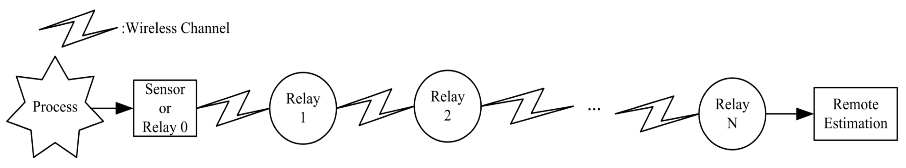
A block diagram of a multi-hop relay network is given in Figure 1. The process is a discrete-time linear system defined on that can be described by
where a discrete time index and . The variables and are state vector and fault signal to be estimated, respectively. The noise signal and is independent identically distributed (i.i.d) , satisfying Gaussian with zero-mean and known variance as follows
The sensor measurement model with both randomly occurring nonlinearity and randomly occurring packet dropouts is described by
where measurement output and measurement noise . It is another i.i.d noise signal satisfying Gaussian with zero-mean and known variance:
where system matrix and output matrix are known with appropriate dimensions. Figure 1 illustrates that the data packets are transmitted to the remote estimator via wireless medium with successive N relay nodes. The current relay node will receive data packets only from its last node then forward data packets to next relay node. The sensor node is treated as relay 0 and other relay nodes are denoted as relay . Additionally, let be the decision variable: if , the data packets in the relay node i will be sent to the next relay node, and if , they will not be sent. The random variables and are Bernoulli-distributed white sequences with the following probabilities.
where are know constants. All random variables and are assumed to be independent in k and uncorrelated with noise signals and . The nonlinear function is further assumed to be known and analytic everywhere. The dynamic model of the fault vector borrowed from [42,43] can be established as follows:
where is a known matrix with appropriate dimensions.
Remark 1.
For the co-design problem of state and fault estimator using stochastic system model, a robust fault estimation filter design was proposed in terms of Riccati-like difference equations in [44,45]. Using the assumption that the sampling interval was sufficiently small, it was supposed that the fault difference item was too small to be neglected. However, in practice, faults always generate a great amplitude change of a certain time, especially when time-varying faults occur. Compared with the assumption in [44,45], it is clear that time-varying fault model described in Equation (6) covers the results of constant faults as a special case, which is less restrictive.
Remark 2.
The measurement model proposed in Equation (3) provides a unified framework to account for the phenomenon of both randomly occurring sensor nonlinearities and random packet dropouts. The stochastic variable is indicated as the phenomenon of the probabilistic sensor nonlinearities, while the random variable is used to represent the nature of random packet dropouts. Specifically, if and , it means that the sensor work normally; if and , it can be seen that the sensor is subject to nonlinearity only; and if , the measurement output contains the noise signal only, implying that the random packet dropouts occur.
Before giving the main results, the following lemma, which will be useful in this paper, needs to be introduced.
Lemma 1.
(Lemma 1 [46]) Let A, D, E and F be real matrices of appropriate dimensions with . For any matrix and scalar such that , then we have
3. Main Results
3.1. A Co-Design Algorithm of Event-Triggered State and Fault Estimator
Based on the measurement mentioned before, the estimated variable of the sensor node (or the relay node 0) can be recursively computed as follows.
where is the estimator gain to be designed. Further, the estimation on the relay node i is suggested as follows:
while the corresponding estimation error covariance is given by
where estimation error , error covariance and .
Remark 3.
Traditionally, the remote estimator needs to know measurements collected by sensors at each time instant k. However, reduction of the number of relay-to-relay transmission actions has been adopted to make the relay nodes extend lifetime and save energy as much as possible. Under this circumstance, multi-hop links may create a problem: the measurements could not be obtained at each time instant and the estimated values could not be calculated by the remote estimator. Because the ultimate goal for remote estimation is to obtain estimated values at each time instant, it follows from Equation (11) that the relay nodes can forward “the estimated” values to the remote estimator.
The purpose of this section is to design an estimator of form Equation (10) for the stochastic system in Equation (1) and the sensor in Equation (3) with incomplete information (randomly occurring sensor nonlinearities and randomly occurring packet dropouts). More specifically, we are interested in looking for the filter parameter such that the following requirements are met simultaneously:
- (a)
- For the phenomenon of packet loss and randomly occurring sensor nonlinearities, an upper bound of the error covariance is derived, i.e., there exists a sequence of positive-definite matrices that satisfies
- (b)
- The sequence of upper bound is minimized by the designed estimator gain through a recursive scheme.
Now we are in a position to obtain an upper bound of the error covariance in the following theorem.
Theorem 1.
Consider the stochastic system described by Equation (1) with measurements in Equation (3) suffering from both packet loss and randomly occurring sensor nonlinearities. For a arbitrary positive constant γ and the given initial condition , if there exists , then the error covariance satisfies
where
with , , , , , , and .
Proof.
First, the error dynamics of the addressed system are calculated by subtracting Equation (1) from Equation (10):
With the help of results in [47] and Taylor series expansion to around , we have
where and represented the first-order term of the Taylor series expansion. Moreover, the high-order term can be changed into the following form:
where is a matrix with appropriate dimension that depends on the problem, is used to accommodate the estimator with a further extent of freedom, and is an unknown discrete-time matrix that stands for the error of linearization of model that requires . Inserting Equations (17) and (18) into Equation (16), the expression of estimation error can be expanded as
By the definition of error covariance , it follows from Equation (16) that
where , , , , , and . According to the initial condition , the upper bound of error covariance can be proved by induction. Let , we need to prove that . Using the elementary inequality and the results of Lemma 1, can be rewritten as
Noticing the facts that , the above Inequality (21) can be rewritten as follows:
Since the assumption that nonlinear function is known and analytic everywhere, we can deduce that is calculable and further derive as the following form
which implies that Inequality (14) is true. ☐
In what follows, the gain matrix is determined by minimizing the upper bound of error covariance given by Equation (14).
Theorem 2.
Consider the stochastic system described by Equation (1) with measurements in Equation (3) suffering from both packet dropouts and randomly occurring sensor nonlinearities. The gain matrix is given as follows
where , , , and . Furthermore, the upper bound of the estimator error covariance is recursively calculated by Riccati-like difference Equation (15).
Proof.
We are ready to show that the gain described by Equation (24) is optimal in the sense that minimizes the upper bound . Note that three terms in Equation (15) are quadratic in . The matrix differentiation formulas may be applied to Equation (15). Now differentiate with respect to . The result is
We set the derivative equal to zero and the optimal gain is solved as follows
with , , , and . which is as same as (24). It is clear that the estimator gain is optimal that minimizes the upper bound for the estimator error covariance. ☐
3.2. Data Forwarding with Packet Dropouts
Thus far, we have derived an upper bound of the estimator error covariance and such an upper bound is subsequently minimized by properly designing the estimator gain. However, as shown in Section 3.1, we only consider the case of data packet dropouts in the sensor transmission stage. The problem on data packet loss is neglected in the multi-hop links. In the following, the mean-square boundedness of the error covariance will be presented.
Theorem 3.
Consider the relay node i and the stochastic system described by Equation (1) subject to random packet loss in the multi-hop links. Let be s-th eigenvalue of matrix A and . If system matrix A is unstable and satisfies , then the error covariance is mean-square bounded, namely, , where Θ is a unique positive solution.
Proof.
The upper bound of the error covariance in the relay node i is updated according to Equations (12) and (14), and then, by taking expectation on both sides, we obtain
The differences of expectations between two adjacent sampling instants can be derived as follows
where the initial condition . According to the considered topology given in Figure 1 and the unstable system matrix A, it is shown that
Then, from the above equalities in Equation (29), we can infer that via the Lemma 2.2 presented in [48], which implies that , where . Utilizing the induction method and the continuity of Equation (27), we can know that , where . Further, let us denote as the steady-state value for in the current relay node i, and is the solution of the following matrix equation.
where . This is equivalent to an extended Lyapunov equation and has a unique positive solution if
As a result, , where is a unique positive solution. It can be concluded that the boundedness and convergence of is guaranteed. ☐
Remark 4.
Remark 5.
Due to the random packet dropouts, the error covariance is time-varying for any given positive initial state. However, is bounded with probability if is bounded [49]. Therefore, with can be considered that the estimation error is mean square stable.
Although many event-triggered sensor schedules (e.g., [50,51]) can be utilized in the multi-hop networks, wireless communication network failures make the relay nodes unable to complete the data-forwarding tasks. Thus, it is necessary to design an energy-efficient data-forwarding scheme for relay nodes against the situation of network data dropouts.
Theorem 4.
Given that a positive constant , if the following event condition of the relay node i
is satisfied, where stands for the absolute value, then the proposed estimator in Equation (11) can ensure that is bounded by , where Ω is a unique positive solution.
Proof.
Let us start to recall the following expression for in Theorem 3
Using the property of matrix trace, the above Equation (33) becomes
For the sequence , we have
where represents the absolute value. Then, substituting the event condition in Equation (32) into Equation (35) yields
The following proof of Theorem 4 is similar to that of Theorem 3. The detailed proof is thus omitted. ☐
| Algorithm 1 Event-triggered data-forwarding scheme |
| At each time instant k, the relay node i executes: initialization and ;
|
We now elaborate this scheme described in Algorithm 1 for relay node i. First of all, the measurements are collected locally at each time instant, then the state values are estimated by a steady-state Kalman filter. Next, the relay node i will forward the estimated state values to the next relay node. If and , the relay node i will successfully receive the estimated state values from relay node at time instant k, i.e., and the corresponding error variance can be calculated as . To achieve more accurate estimates of system state, the relay node i will forward data packets to the next relay node without entering the event-triggered decision rule. Whereas, if or at time instant k, relay node will not send the estimated state values to relay node i for energy conservation (or relay node i cannot receive the data packets due to data losses). Without state information from relay node , the estimated state values and error variance at relay node i will be updated as follows: , and . Then, the event-triggered decision rule will determine whether the relay node i will send the current estimated state value to the next relay node.
4. Experimental Verification
In this section, the effectiveness of the proposed theoretical algorithm will be evaluated on a test bed that is a scale-down industrial process of twin water tanks. Based on the architecture of Figure 1, a sensor node (Node 1) and two relay nodes (Node 2 and Node 3) are designed to construct a multi-hop network transmitting water level information from Node 1 to Node 2 and to Node 3. At Node 3, the information on water level will be fed to a remote computer. This section is organized as follows. A new transmission protocol including the implementation of hardware and the corresponding procedure is presented in Section 4.1. Section 4.2 introduces system description and modeling. Experimental results on estimation quality and energy conservation are obtained in Section 4.3.
To verify the effectiveness of our proposed data-forwarding scheme, we shall present a new transmission protocol in the following section.
4.1. A New Transmission Protocol for Data Forwarding Scheme
In the most industrial applications, a wireless transmission module (WTM) always consumes more energy than a computation module. This is why we have designed data-forwarding scheme to reduce the amount of time for sending and receiving data, making the lifetime of the wireless node longer. However, stopping communication does not mean stopping energy consumption. It is because the WTM of each node keeps monitoring whether the data has arrived or not. Although the characteristic of the WTM can make it sleep to achieve the result of energy conservation in the single-hop wireless networks [52], the wireless transmission technology may not allow us to obtain such a sleeping capability in the multi-hop networks. For example, two nodes including station (STA) mode and access point (AP) mode have been embedded in the Wi-fi technology and they have to exist in the relay node. However, the WTM chosen as AP mode will spend a lot of time waking up (or even cannot wake up) once it enters a sleep state. It will extend the transmission time and lead to limited applications in real-world applications. The ZigBee communication technology cannot be applied to the network topology described in Figure 1 because the coordinator and router, which have to be added as a relay node in the multi-hop network, cannot go to sleep. In addition, the Bluetooth technique is not qualified as the WTM of relay nodes due to its long matching time and limited transmission distance. All of these motivate us to come up with a new transmission protocol suitable for any data-forwarding schemes in multi-hop relay networks.
First, we introduce the components of each relay node: (i) the wireless transmission module forwards the data packets between the relay nodes; (ii) the computation module determines when to forward data packets via our forwarding scheme; (iii) the switching module turns off and on the power of WTM; and (iv) the transmitter and receiver are a pair of wireless transceivers to distinguish them from the WTM. The transmitter and receiver are used as a medium to wake up WTM quickly and to ensure the network connectivity when the WTM is commanded into a sleep mode.
The procedure of this new transmission protocol is now presented in Algorithm 2.
| Algorithm 2 The implementation steps for the new transmission protocol |
| When the data packet is requested to be sent from the relay node i to the relay node , the following steps are performed: Step 1: For relay node i, the computation module sends a specified digital signal to the transmitter through I/O ports. Step 2: For relay node i, the switching module turns on the power of WTM. Step 3: The transmitter of relay node i sends a signal to the receiver of relay node . Step 4: For relay node , the receiver sends a specified digital signal to wake up the computation module by I/O ports. Step 5: For relay node , the computation module requires switching module to power on the WTM. Step 6: The WTM of relay node i forwards data packets to the WTM of relay node . Step 7: For relay node i, the switching module turns off the power of WTM after the end of transmission. end |
4.1.1. Hardware Design for the Experiment
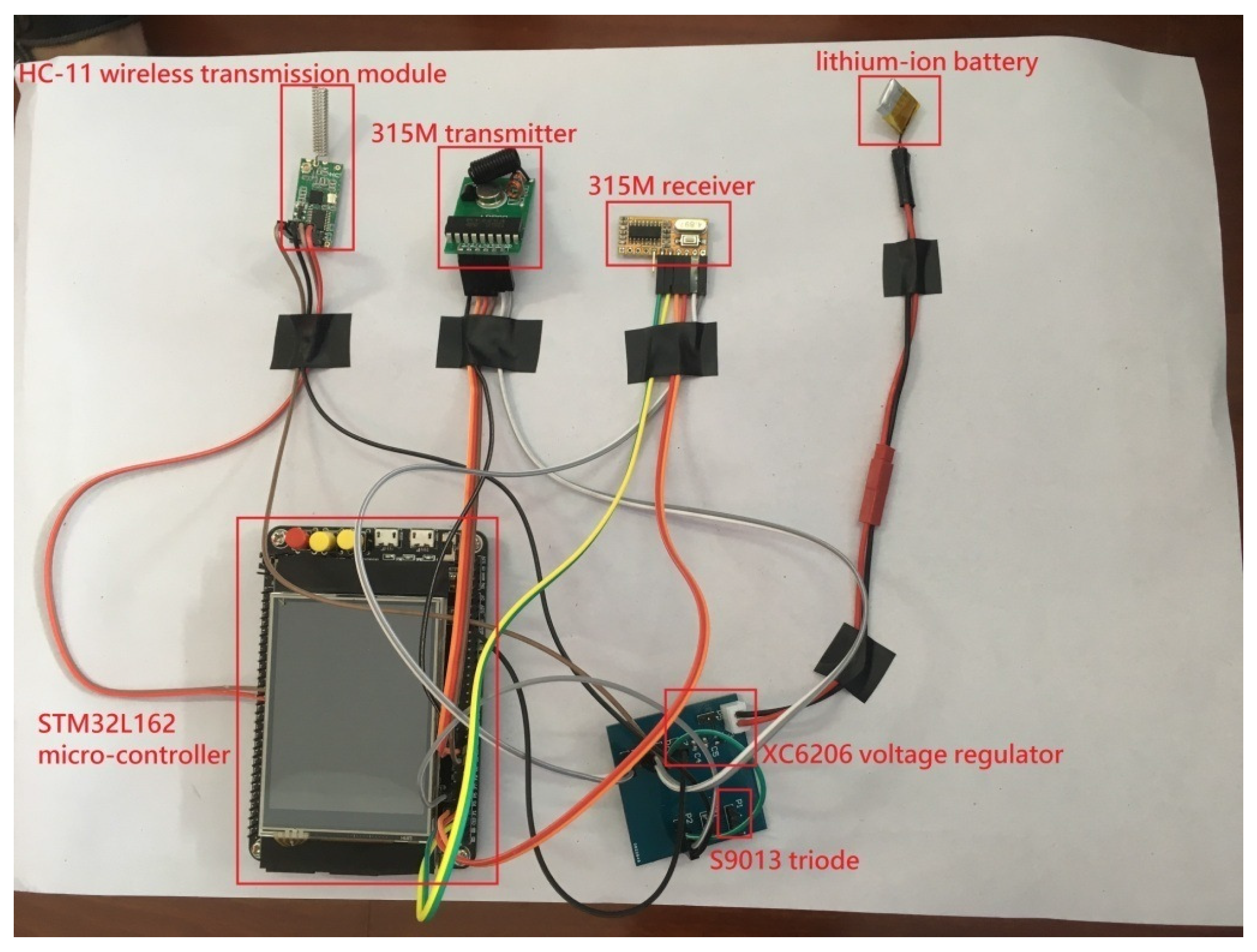
Node 1 acts as the head node, Nodes 2 and 3 together construct a multi-hop network for verification of our theoretical results in this experiment. The physical connection diagram in Figure 2 is a photograph of the components in Node 2. Due to the limited space in this paper, the structures of Node 1 and Node 3 are omitted. They are similar to the structure of Node 1 except that the receiver and transmitter ignored in the Node 1 and Node 3, respectively. As shown in Figure 2, the node contains the following components: an STM32L162ZD micro-controller [53] (STM32, Geneva, Switzerland) including an ARM cortexTM-M3 CPU, a 384 Kbytes Flash memory, and a 48 Kbytes RAM that allows us to use it as a computation module; and an HC-11 [54] (also called 433 Mhz UART serial wireless transceiver module) with simple and flexible operation is selected as the WTM. Furthermore, the corresponding switching module is an S9013 NPN type triode and the power management system is composed of an X6206 voltage regulator and a Lithium-ion battery. In particular, the reason why we choose 315M transmitter and receiver is due to their extreme low power consumption. Even though its transmission rate is very limited, the electric current of idle state is approximately 0 mA, and the electric current in transmission state is lower than 2 mA.
4.1.2. Implementation of the Experiment
To implement this experiment, two scenarios will be discussed in Algorithms 3 and 4. If the transmission commands are calculated by the STM32 using our designed forwarding scheme, the active mode is executed and the sleep mode is activated otherwise.
| Algorithm 3 The active mode for Node i |
| When Node i sends the data packet to Node , the following steps will be performed: Step 1: For Node i: STM32 sends a signal to 315M transmitter and activates HC-11. Step 2: For Node : 315M receiver activates STM32 then activates HC-11. Step 3: Node i forwards data packets to Node . Step 4: For Node i: turns off HC-11. end |
| Algorithm 4 The sleep mode for Node i |
| When Node i is not allowed to send the data packet to Node , the following steps will be performed: Step 1: For Node i: STM32 and 315M transmitters enter an idle state and the HC-11 is not turned on. Step 2: For Node : STM32 calculates the corresponding decision to determine whether or not sending data packets based on the proposed data-forwarding scheme. The 315M receiver enters an idle state then HC-11 is not turned on. end |
Additionally, the received data packets may contain incomplete data packets (or data packets with error information) due to network failures, so a data validation algorithm is presented in Algorithm 5 which also reduce the probability of data-packet loss to some extent. We now introduce two indicators and . Either or , the re-transmission commands sent by Node 2 (or Node 3) will be fed back to Node 1 (or Node 2). Conversely, both and , the end command will be executed.
| Algorithm 5 Data validation |
| When sending the data packets from Node 1 to Node 2 (or from Node 2 to Node 3), the following procedures will be executed: initialization ;
|
4.2. System Description and Modeling of the Twin Water-Tank System
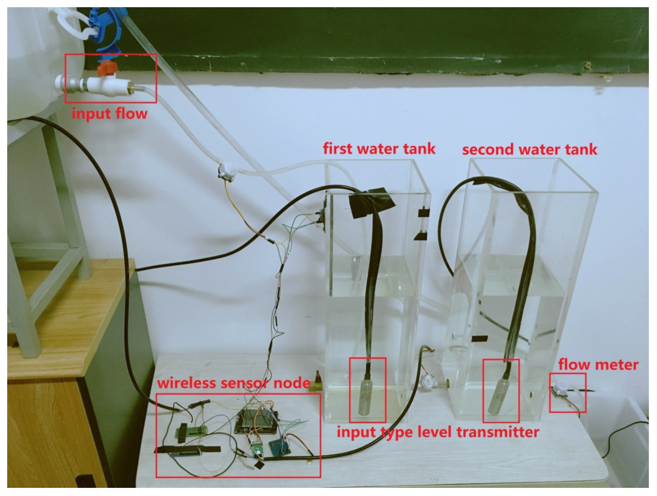
In this subsection, the feasibility and practicality of the proposed theoretical results and the transmission protocol will be examined on a continuous-time linear model [55]. Figure 3 is a photograph of the architecture of the twin water-tank system including two small tanks and a reservoir. The system state-space equations are described as follows.
where for and 2, is the water level and can be calculated using the sensor’s measurements where is voltage values measured by the input-type level transmitter placed in each tank. The flow rate can be calculated as and where and are measured by the flow meters. In addition, and are the cross-sectional areas of the water tanks, and and are water resistance. Furthermore, and are output variables satisfying the following relationship
Based on parameters of the experimental platform, the discretized model of the system in Equation (37) with a sample of 5 s is formulated as follows
where the noise processes and are assumed mutually independent, white, zero-mean and have known variance and , respectively. The error accuracy of the level transmitters is centimeters. Considering the main technical specifications of water level sensors, the following parameters are chosen as , . The nonlinear function and formulate the first-order expansion term coefficient with the high-order expansion term .
4.3. Assessment of Effectiveness of the Theoretical Results
In this part, the effectiveness of the proposed estimator and data-forwarding scheme will be assessed through the following experiments.
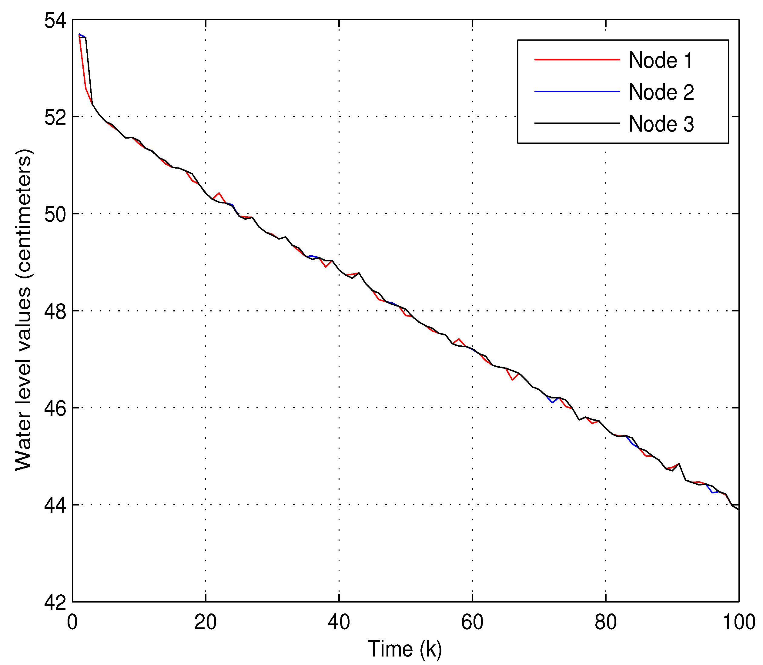
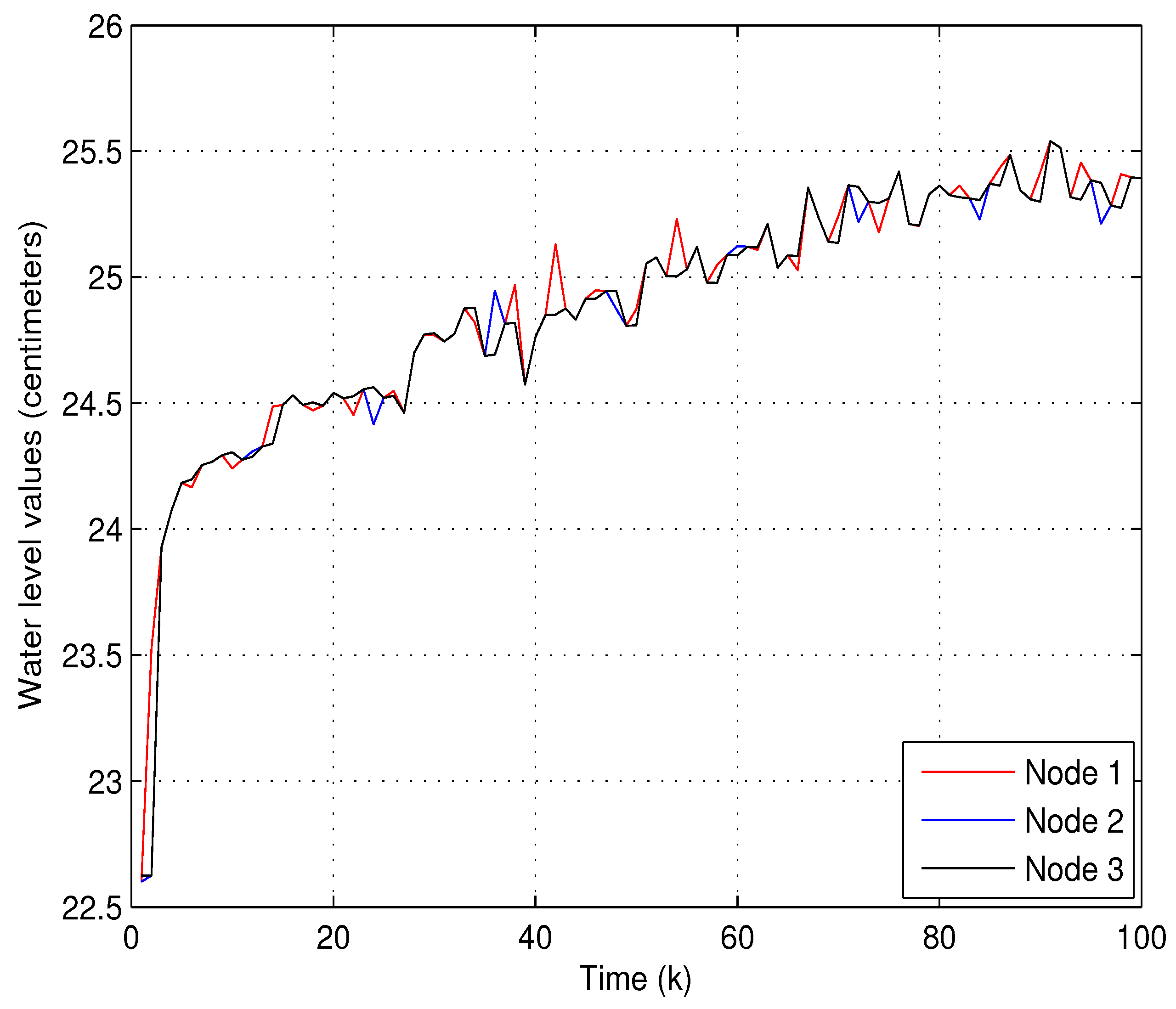
(1) Experiment 1: In the first experiment, the accuracy of state estimation will be evaluated by using the proposed data-forwarding scheme. we temporarily ignore system fault in system Equation (1) for the convenience of discussion. The running times of this system is set to 50, and the initial water level of the twin water tanks are 53 and 24 centimeters, respectively. To verify the practicability of the proposed algorithm, the following parameters are set as (i = 1 and 2), , , and the transmission threshold (i= 1 and 2). Figure 4 and Figure 5 show that two water levels measured by the level transmitters and the estimated water levels of each node via our proposed estimator and data-forwarding scheme. As shown in Figure 4 and Figure 5, the measured values and the estimated values are coincident as time increases. Obviously, the estimation accuracy is satisfactory using the proposed data transmission scheme. Moreover, the corresponding communication behaviors on , and at each time instant are demonstrated in Figure 6. It can be also noted that our data-forwarding scheme can effectively reduce the update frequency as compared with the traditional time-triggered mechanism.
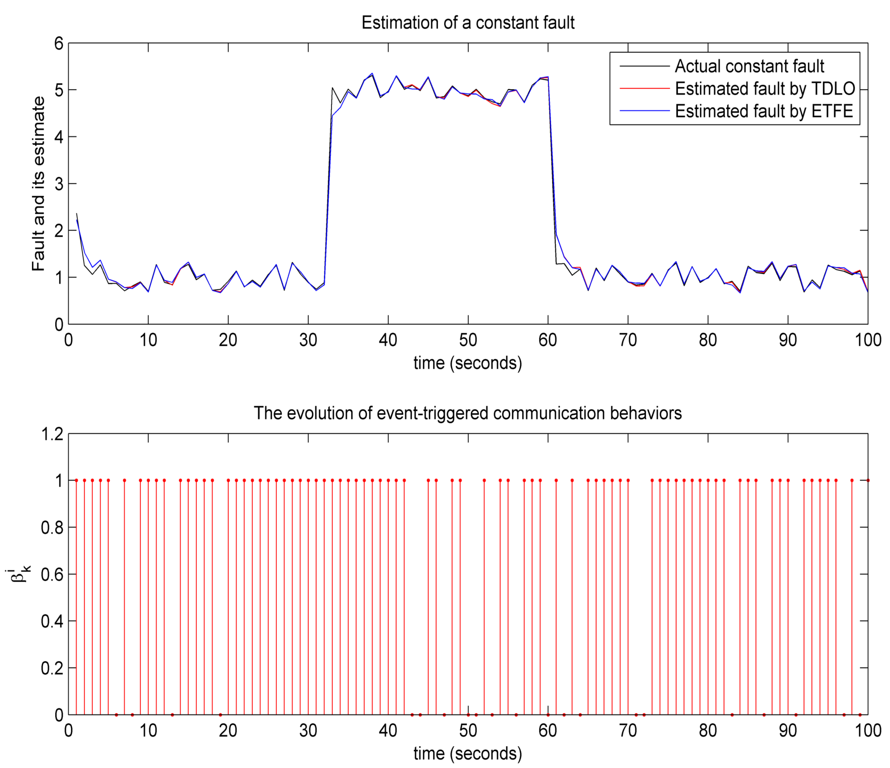
(2) Experiment 2: To verify the performance of event-triggered fault estimation, the following fault scenarios are used to complete our second experiment. A constant fault
and a time-varying fault
The estimated signals of a constant fault and a time-varying fault are illustrated in Figure 7 and Figure 8, respectively. As comparison, fault-estimating signals using the time-driven learning observer (TDLO) borrowed from [4] and the evolution of event-triggered communication behaviors are also depicted Figure 7 and Figure 8. It is worth mentioning that, compared with TDLO, the proposed event-triggered fault estimation (ETFE) not only provides better rapidity of fault estimation but also achieves robust reconstruction of the constant and time-varying actuator faults. Further, we examine the effect on the estimation performance from the different and (i= 1 and 2) in Table 1 and Table 2, respectively. We can also find that a larger probability corresponds to a smaller error bound, that is, when randomly sensor nonlinearity and packet dropout have smaller probabilities of occurring, the fault estimation can achieve a better performance. All of these make it possible for the ETFE to be easily implemented in practice.
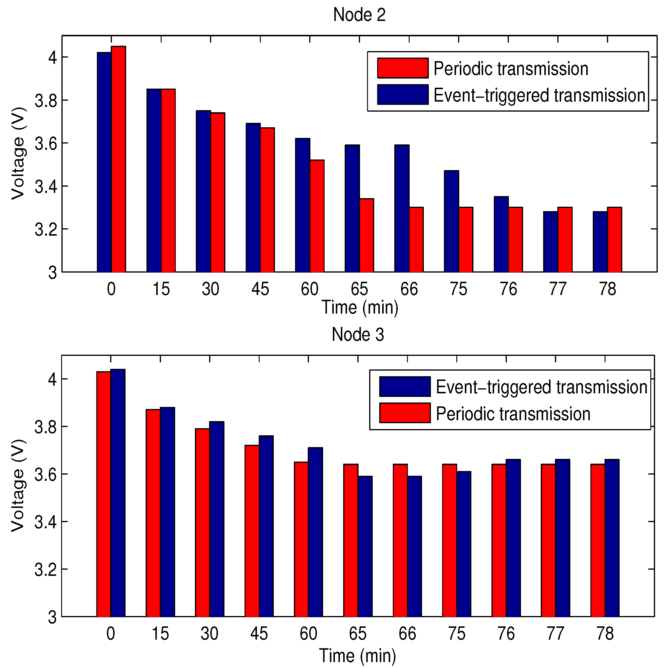
(3) Experiment 3: Here, the energy conservation is now verified using a 50 mAh battery. The comparison of battery voltage at Node 2 and Node 3 are illustrated by Figure 9 where the battery voltage using the periodically forwarding scheme drops to 3.28 V after 66 min. Node 2 cannot work normally because its working voltage must exceed 3.3 V [53]. Comparatively, the battery voltage at Node 2 using the VDFS reaches 3.3 V after 77 min. We find that Node 2 consumed more energy than other nodes. The reason is that the 315M transmitter and receiver are installed at Node 2 and they can consume more energy. Because the network topology described in Figure 1 is fixed, the system stop operating once the battery at Node 2 is completely consumed. The working life of the battery is prolonged by 16.7%.
5. Conclusions and Further Work
In this work, we have addressed the co-design problem of state and fault estimation with an event-triggered data-forwarding scheme against both randomly occurring nonlinearity and randomly occurring packet dropouts governed by Bernoulli-distributed sequences in multi-hop relay wireless networks. Recursive Riccati-like matrix equations are established to calculate the estimator gain in order to minimize an upper bound of error covariance. A Sufficient condition and a data-forwarding scheme have been derived to achieve the mean-square boundedness of the error covariance in the multi-hop relay links with random packet dropouts. Such data-forwarding scheme enables each relay node to forward the estimated values to the remote estimator. Furthermore, a new transmission protocol can be applied to the desired event-triggered transmission scheme under the fixed network topology where a relay node has the knowledge of its previous relay node and of next relay node. The effectiveness of the proposed technique has been evaluated by using a twin water-tank system with a sensor and two relay nodes.
However, we also find some open problems that should be solved in future research. First, time delays should be considered in this kind of network topology. The constant (or random) time delays can occur if the number of relays are large. Next, a switching module S9013 has been used for turning the wireless transmission module on and off. However, the wireless transmission module may reduce the operating life due to frequent opening and closing. It is necessary that the wireless transmission module implement self-dormancy for energy saving. Finally, combing event-triggered transmission scheme and coding technologies may be an interesting direction for improving energy conservation in multi-hop relays networks.
Acknowledgments
This work is supported by Education Ministry and China Mobile Science Research Foundation: Video Big Data Analysis and IoT Interaction Technology Research (MCM20170204).
Author Contributions
In this work, Yunji Li conceived, designed, performed, and analyzed the experiments and wrote the paper under the guidance of Li Peng.
Conflicts of Interest
The authors declare no conflicts of interest.
References
- Rashvand, H.F.; Abedi, A.; Alcaraz-Calero, J.M.; Mitchell, P.D.; Mukhopadhyay, S.C. Wireless sensor systems for space and extreme environments: A review. IEEE Sens. J. 2014, 14, 3955–3970. [Google Scholar] [CrossRef]
- Niu, Y.; Ho, D.W.C.; Li, C.W. Filtering for discrete fuzzy stochastic systems with sensor nonlinearities. IEEE Trans. Fuzzy Syst. 2010, 18, 971–978. [Google Scholar] [CrossRef]
- Jia, Q.; Chen, W.; Zhang, Y.; Li, H. Fault reconstruction and fault-tolerant control via learning observers in Takagi-Sugeno fuzzy descriptor systems with time delays. IEEE Trans. Ind. Electron. 2015, 62, 3885–3895. [Google Scholar] [CrossRef]
- Chen, W.; Chen, W.T.; Saif, M.; Li, M.F.; Wu, H. Simultaneous Fault Isolation and Estimation of Lithium-Ion Batteries via Synthesized Design of Luenberger and Learning Observers. IEEE Trans. Control Syst. Technol. 2014, 22, 290–298. [Google Scholar] [CrossRef]
- Ovsthus, K.; Kristensen, L.M. An industrial perspective on wireless sensor networks—A survey of requirements, protocols, and challenges. IEEE Commun. Surv. Tutor. 2014, 16, 1391–1412. [Google Scholar] [CrossRef]
- Zhang, L.; Gao, H.; Kaynak, O. Network-induced constraints in networked control systems—A survey. IEEE Trans. Ind. Inform. 2013, 9, 403–416. [Google Scholar] [CrossRef]
- Zhang, X.M.; Han, Q.L.; Yu, X. Survey on recent advances in networked control systems. IEEE Trans. Ind. Inform. 2016, 12, 1740–1752. [Google Scholar] [CrossRef]
- Zhang, X.M.; Han, Q.L. Network-based H∞ filtering using a logic jumping-like trigger. Automatica 2013, 49, 1428–1435. [Google Scholar] [CrossRef]
- Patton, R.J.; Chen, J. Observer-based fault detection and isolation: Robustness and applications. Control Eng. Pract. 1997, 5, 671–682. [Google Scholar] [CrossRef]
- Xiong, Y.; Saif, M. Unknown disturbance inputs estimation based on a state functional observer design. Automatica 2003, 39, 1389–1398. [Google Scholar] [CrossRef]
- Alavi, S.M.M.; Saif, M. Fault detection in nonlinear stable systems over lossy networks. IEEE Trans. Control Syst. Technol. 2013, 21, 2129–2142. [Google Scholar] [CrossRef]
- Zhang, Y.; Chen, W.; Chen, X.; Jia, Q. Robust fault reconstruction via learning observers in linear parameter-varying systems subject to loss of actuator effectiveness. IET Control Theory Appl. 2014, 8, 42–50. [Google Scholar] [CrossRef]
- Shi, P.; Zhang, Y.; Chadli, M.; Agarwal, R.K. Mixed H-Infinity and Passive Filtering for Discrete Fuzzy Neural Networks With Stochastic Jumps and Time Delays. IEEE Trans. Neural Netw. Learn. Syst. 2016, 27, 903–909. [Google Scholar] [CrossRef] [PubMed]
- Chadli, M.; Abdo, A.; Ding, S.X. H−/H∞ fault detection filter design for discrete-time Takagi-Sugeno fuzzy system. Automatica 2013, 49, 1996–2005. [Google Scholar] [CrossRef]
- Chen, W.; Saif, M. An iterative learning observer for fault detection and accommodation in nonlinear time-delay systems. Int. J. Robust Nonlinear Control 2006, 16, 1–19. [Google Scholar] [CrossRef]
- Youssef, T.; Chadli, M.; Karimi, H.R.; Wang, R. Actuator and sensor faults estimation based on proportional integral observer for TS fuzzy model. J. Frankl. Inst. 2017, 354, 2524–2542. [Google Scholar] [CrossRef]
- Li, F.; Shi, P.; Lim, C.C.; Wu, L. Fault detection filtering for nonhomogeneous markovian jump systems via fuzzy approach. IEEE Trans. Fuzzy Syst. 2017, 26, 131–141. [Google Scholar] [CrossRef]
- Chibani, A.; Chadli, M.; Braiek, N.B. A sum of squares approach for polynomial fuzzy observer design for polynomial fuzzy systems with unknown inputs. Int. J. Control Autom. Syst. 2016, 14, 323–330. [Google Scholar] [CrossRef]
- Chen, W.; Chowdhury, F.N. Simultaneous identification of time-varying parameters and estimation of system states using iterative learning observers. Int. J. Syst. Sci. 2007, 38, 39–45. [Google Scholar] [CrossRef]
- Jia, Q.; Chen, W.; Zhang, Y.; Chen, X. Fault Reconstruction and Accommodation in Linear Parameter-Varying Systems via Learning Unknown-Input Observers. J. Dyn. Syst. Meas. Control 2015, 137, 0610081–0610089. [Google Scholar] [CrossRef]
- Chibani, A.; Chadli, M.; Peng, S.; Braiek, N.B. Fuzzy fault detection filter design for t-s fuzzy systems in finite frequency domain. IEEE Trans. Fuzzy Syst. 2017, 25, 1051–1061. [Google Scholar] [CrossRef]
- NaNacara, W.; Yaz, E.E. Recursive estimator for linear and nonlinear systems with uncertain observations. Signal Process. 1997, 62, 215–228. [Google Scholar] [CrossRef]
- Wang, Z.; Shen, B.; Liu, X. H∞ filtering with randomly occurring sensor saturations and missing measurements. Automatica 2012, 48, 556–562. [Google Scholar] [CrossRef]
- Wu, Z.G.; Shi, P.; Su, H.; Chu, J. Asynchronous ℓ2-ℓ∞ filtering for discrete-time stochastic Markov jump systems with randomly occurred sensor nonlinearities. Automatica 2014, 50, 180–186. [Google Scholar] [CrossRef]
- Miskowicz, M. Send-on-delta concept: An event-based data reporting strategy. Sensors 2006, 6, 49–63. [Google Scholar] [CrossRef]
- Suh, Y.S.; Nguyen, V.H.; Ro, Y.S. Modified Kalman filter for networked monitoring systems employing a send-on-delta method. Automatica 2007, 43, 332–338. [Google Scholar] [CrossRef]
- Mao, J.; Ding, D.; Song, Y.; Liu, Y.; Alsaadi, F.E. Event-based recursive filtering for time-delayed stochastic nonlinear systems with missing measurements. Signal Process. 2017, 134, 158–165. [Google Scholar] [CrossRef]
- Meng, X.; Chen, T. Optimality and stability of event triggered consensus state estimation for wireless sensor networks. In Proceedings of the American Control Conference, Portland, OR, USA, 4–6 June 2014; pp. 3565–3570. [Google Scholar]
- Heemels, W.P.M.H.; Johansson, K.H.; Tabuada, P. An introduction to event-triggered and self-triggered control. In Proceedings of the IEEE Conference on Decision and Control, Maui, HI, USA, 10–13 December 2012; pp. 3270–3285. [Google Scholar]
- Lunze, J. Event-Based Control: Introduction and Survey. In Event-Based Control and Signal Processing; CRC Press: Boca Raton, FL, USA, 2015; pp. 3–20. [Google Scholar]
- Chen, T.; Meng, X. Event triggered robust filter design for discrete-time systems. IET Control Theory Appl. 2014, 8, 104–113. [Google Scholar] [CrossRef]
- Meng, X.; Chen, T. Event-based stabilization over networks with transmission delays. J. Control Sci. Eng. 2012. [Google Scholar] [CrossRef]
- Han, D.; Mo, Y.; Wu, J.; Weerakkody, S.; Sinopoli, B.; Shi, L. Stochastic event-triggered sensor schedule for remote state estimation. IEEE Trans. Autom. Control 2015, 60, 2661–2675. [Google Scholar] [CrossRef]
- Diazcacho, M.; Delgado, E.; Barreiro, A.; Falcón, P. Basic send-on-delta sampling for signal tracking-error reduction. Sensors 2017, 17, 312. [Google Scholar] [CrossRef] [PubMed]
- Socas, R.; Dormido, S.; Dormido, R.; Fabregas, E. Event-based control strategy for mobile robots in wireless environments. Sensors 2015, 15, 30076–30092. [Google Scholar] [CrossRef] [PubMed]
- Socas, R.; Dormido, R.; Dormido, S. New Control Paradigms for Resources Saving: An Approach for Mobile Robots Navigation. Sensors 2018, 18, 281. [Google Scholar] [CrossRef] [PubMed]
- Putra, P.E.S.; Brusey, J.; Gaura, E.; Vesilo, R. An Event-Triggered Machine Learning Approach for Accelerometer-Based Fall Detection. Sensors 2018, 18, 20. [Google Scholar] [CrossRef] [PubMed]
- Xu, Z.; Liu, G.; Yan, H.; Cheng, B.; Lin, F. Trail-based search for efficient event report to mobile actors in wireless sensor and actor networks. Sensors 2017, 17, 2468. [Google Scholar] [CrossRef] [PubMed]
- Santos, C.; Martínez-Rey, M.; Espinosa, F.; Gardel, A.; Santiso, E. Event-based sensing and control for remote robot guidance: An experimental case. Sensors 2017, 17, 2034. [Google Scholar] [CrossRef] [PubMed]
- Acho, L. Event-driven observer-based smart-sensors for output feedback control of linear systems. Sensors 2017, 17, 2028. [Google Scholar] [CrossRef] [PubMed]
- Ravankar, A.; Ravankar, A.A.; Kobayashi, Y.; Emaru, T. Symbiotic navigation in multi-robot systems with remote obstacle knowledge sharing. Sensors 2017, 17, 1581. [Google Scholar] [CrossRef] [PubMed]
- Dong, H.; Wang, Z.; Ding, S.X.; Gao, H. Finite-horizon estimation of randomly occurring faults for a class of nonlinear time-varying systems. Automatica 2014, 50, 3182–3189. [Google Scholar] [CrossRef]
- Dong, H.L.; Wang, Z.D.; Ding, S.X.; Gao, H.J. On H-infinity Estimation of Randomly Occurring Faults for A Class of Nonlinear Time-Varying Systems with Fading Channels. IEEE Trans. Autom. Control 2016, 61, 479–484. [Google Scholar] [CrossRef]
- Chang, J.L. Applying discrete-time proportional integral observers for state and disturbance estimations. IEEE Trans. Autom. Control 2005, 51, 814–818. [Google Scholar] [CrossRef]
- Hu, J.; Liu, S.; Ji, D.; Li, S. On co-design of filter and fault estimator against randomly occurring nonlinearities and randomly occurring deception attacks. Int. J. Gen. Syst. 2016, 45, 619–632. [Google Scholar] [CrossRef]
- Yue, D. Robust stabilization of uncertain systems with unknown input delay. Automatica 2004, 40, 331–336. [Google Scholar] [CrossRef]
- Calafiore, G. Reliable localization using set-valued nonlinear filters. IEEE Trans. Syst. Man Cybern. Part A Syst. Hum. 2005, 35, 189–197. [Google Scholar] [CrossRef]
- Shi, L.; Johansson, K.H.; Qiu, L. Time and event-based sensor scheduling for networks with limited communication resources. IFAC Proc. Vol. (IFAC-PapersOnline) 2011, 44, 13263–13268. [Google Scholar] [CrossRef]
- Schenato, L. Optimal estimation in networked control systems subject to random delay and packet drop. IEEE Trans. Autom. Control 2008, 53, 1311–1317. [Google Scholar] [CrossRef]
- Li, S.; Sauter, D.; Xu, B. Fault isolation filter for networked control system with event-triggered sampling scheme. Sensors 2011, 11, 557–572. [Google Scholar] [CrossRef] [PubMed]
- Li, Y.; Li, P.; Chen, W. An energy-efficient data transmission scheme for remote state estimation and applications to a water-tank system. ISA Trans. 2017, 70, 494–501. [Google Scholar] [CrossRef] [PubMed]
- USR-C322 User Manual, USR IOT Experts. 2017. Available online: http://www.usriot.com/p/ti-cc3200-wifi-modules/ (accessed on 17 May 2017).
- STM32 Reference Manual, STMicroelectronics. 2017. Available online: http://www.st.com/content/stcom/en/products/microcontrollers/stm32-32-bit-arm-cortex-mcus/stm32l1-series/stm32l162/stm32l162zd.html (accessed on 22 January 2017).
- HC-11 Reference Manual. 2017. Available online: https://www.elecrow.com/download/HC-11.eps (accessed on 22 January 2017).
- Versteeg, H.K.; Malaskekera, W. An Introduction to Computational Fluid Dynamics; Pearson Education Limited: London, UK, 2007; ISBN 9780131274983. [Google Scholar]
Figure 1.
A block diagram of the system model.

Figure 2.
The physical connection diagram of Node 2.

Figure 3.
The components of twin water-tanks.

Figure 4.
The measured and the estimated water level values for the first water tank.

Figure 5.
The measured and the estimated water level values for the second water tank.

Figure 6.
The communication behaviors on , and .
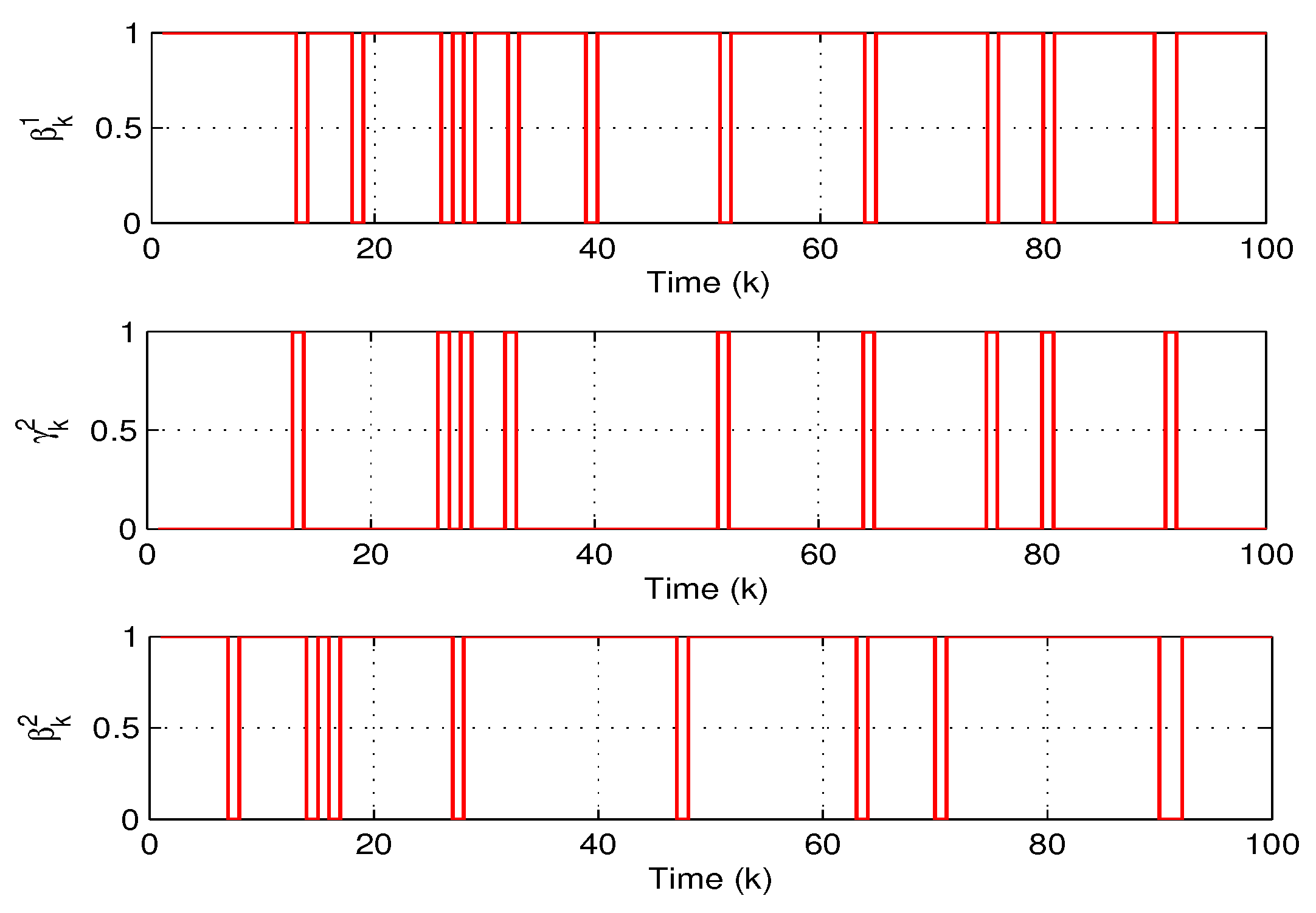
Figure 7.
Reconstruction of a constant fault.

Figure 8.
Reconstruction of a time-varying fault.
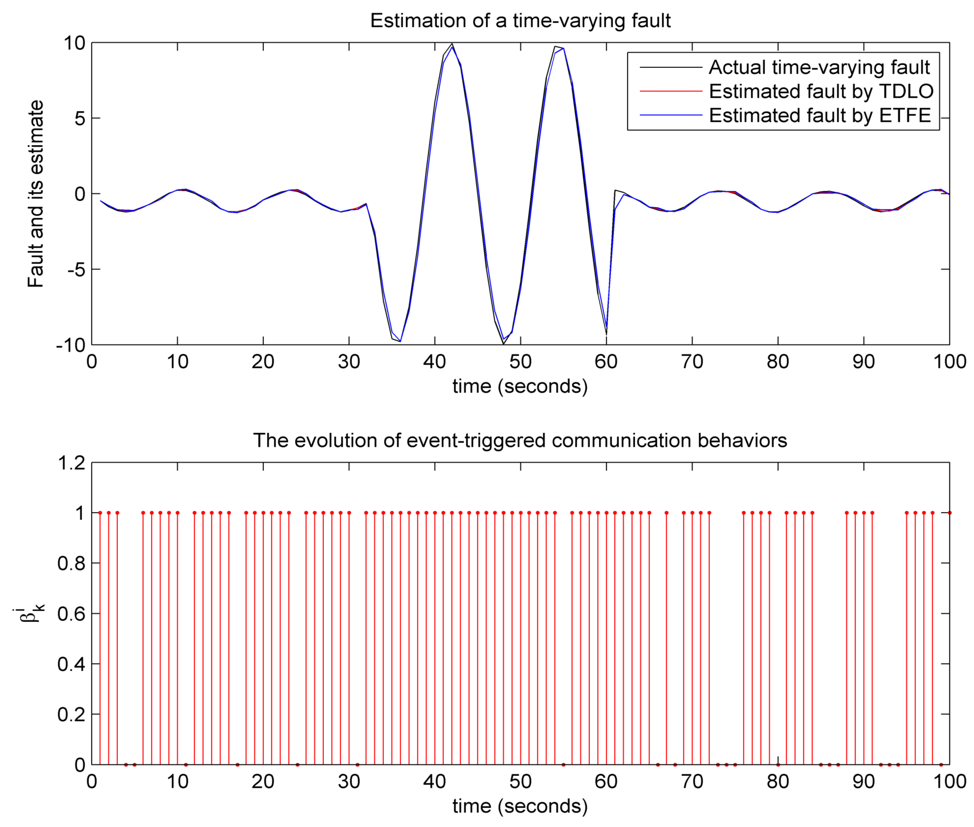
Figure 9.
The comparison of battery voltage for Node 2 and Node 3.


Table 1.
Upper bound of fault estimation error covariance with different for .
| 0.12 | 0.16 | 0.22 | 0.26 | 0.32 | 0.36 | 0.42 | 0.46 | |
| An upper bound of error covariance | 0.231 | 0.24 | 0.373 | 0.381 | 0.396 | 0.412 | 0.438 | 0.466 |
Table 2.
Upper bound of fault estimation error covariance with different for .
| (i = 1 and 2) | 0.12 | 0.16 | 0.22 | 0.26 | 0.32 | 0.36 | 0.42 | 0.46 |
| An upper bound of error covariance | 0.315 | 0.362 | 0.397 | 0.416 | 0.478 | 0.503 | 0.612 | 0.681 |
© 2018 by the authors. Licensee MDPI, Basel, Switzerland. This article is an open access article distributed under the terms and conditions of the Creative Commons Attribution (CC BY) license (http://creativecommons.org/licenses/by/4.0/).
Share and Cite
MDPI and ACS Style
Li, Y.; Peng, L. Event-Triggered Fault Estimation for Stochastic Systems over Multi-Hop Relay Networks with Randomly Occurring Sensor Nonlinearities and Packet Dropouts. Sensors 2018, 18, 731. https://doi.org/10.3390/s18030731
AMA Style
Li Y, Peng L. Event-Triggered Fault Estimation for Stochastic Systems over Multi-Hop Relay Networks with Randomly Occurring Sensor Nonlinearities and Packet Dropouts. Sensors. 2018; 18(3):731. https://doi.org/10.3390/s18030731
Chicago/Turabian StyleLi, Yunji, and Li Peng. 2018. "Event-Triggered Fault Estimation for Stochastic Systems over Multi-Hop Relay Networks with Randomly Occurring Sensor Nonlinearities and Packet Dropouts" Sensors 18, no. 3: 731. https://doi.org/10.3390/s18030731
Note that from the first issue of 2016, this journal uses article numbers instead of page numbers. See further details here.