Facile Quantification and Identification Techniques for Reducing Gases over a Wide Concentration Range Using a MOS Sensor in Temperature-Cycled Operation

Abstract
:1. Introduction
2. Materials and Methods
- (i).
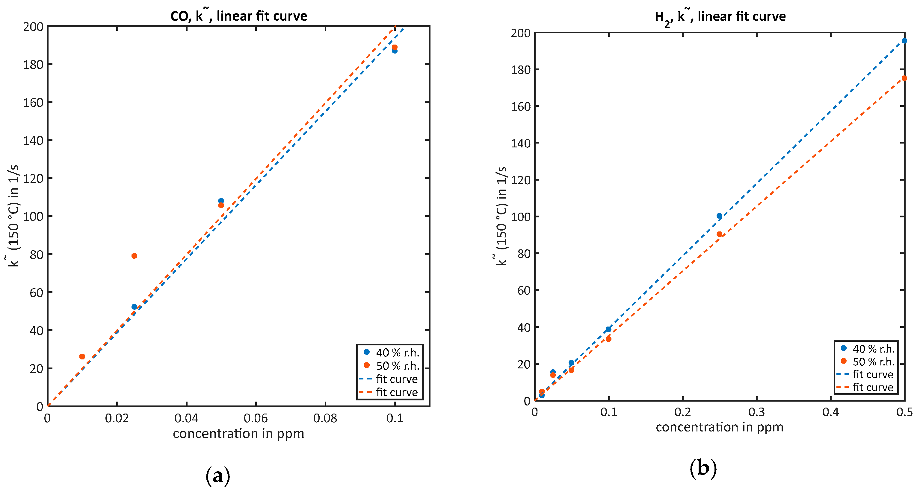
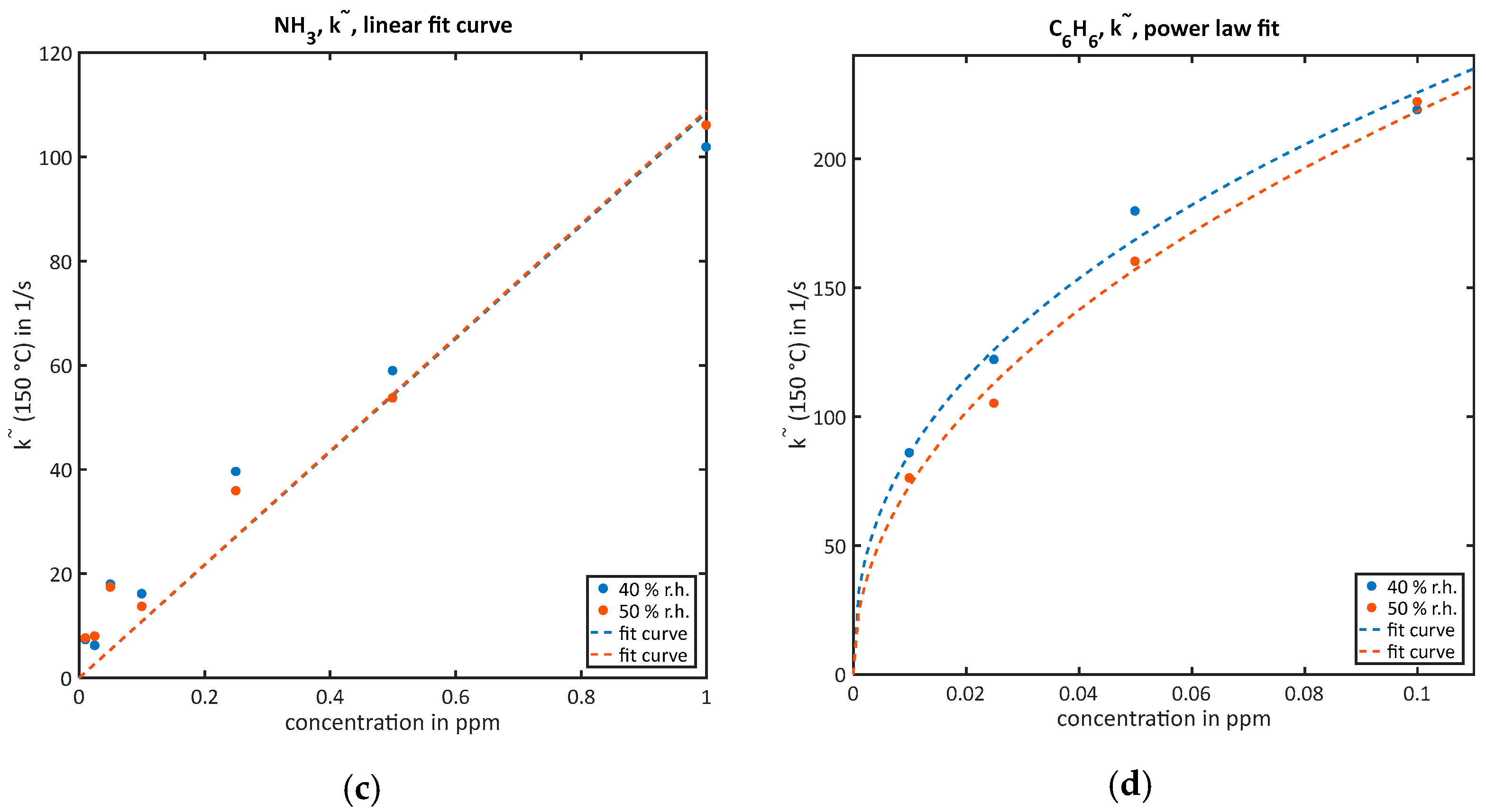
- For the quantification of low concentrations when the sensor does not approach equilibrium of surface coverage during the low-temperature phase, the rate constant is estimated by the calculation of which denotes the slope of . Following the line of [17], is calculated by a linear fit of at the beginning of the low-temperature range. According to Equation (3), the reaction rate constant k and, furthermore, linear to the concentration [17]. The proportionality factor f between and can be calculated using the initial surface coverage at low temperature [17]:However, as the calculated feature is calibrated with the measurement results and the calculation is much more complex than one single linear fit, the explicit calculation of will be omitted for most of the measurements except for one explicit comparison in Section 4. To compensate the background, the slope of zero air is subtracted from all calculated values [17].
- (ii).
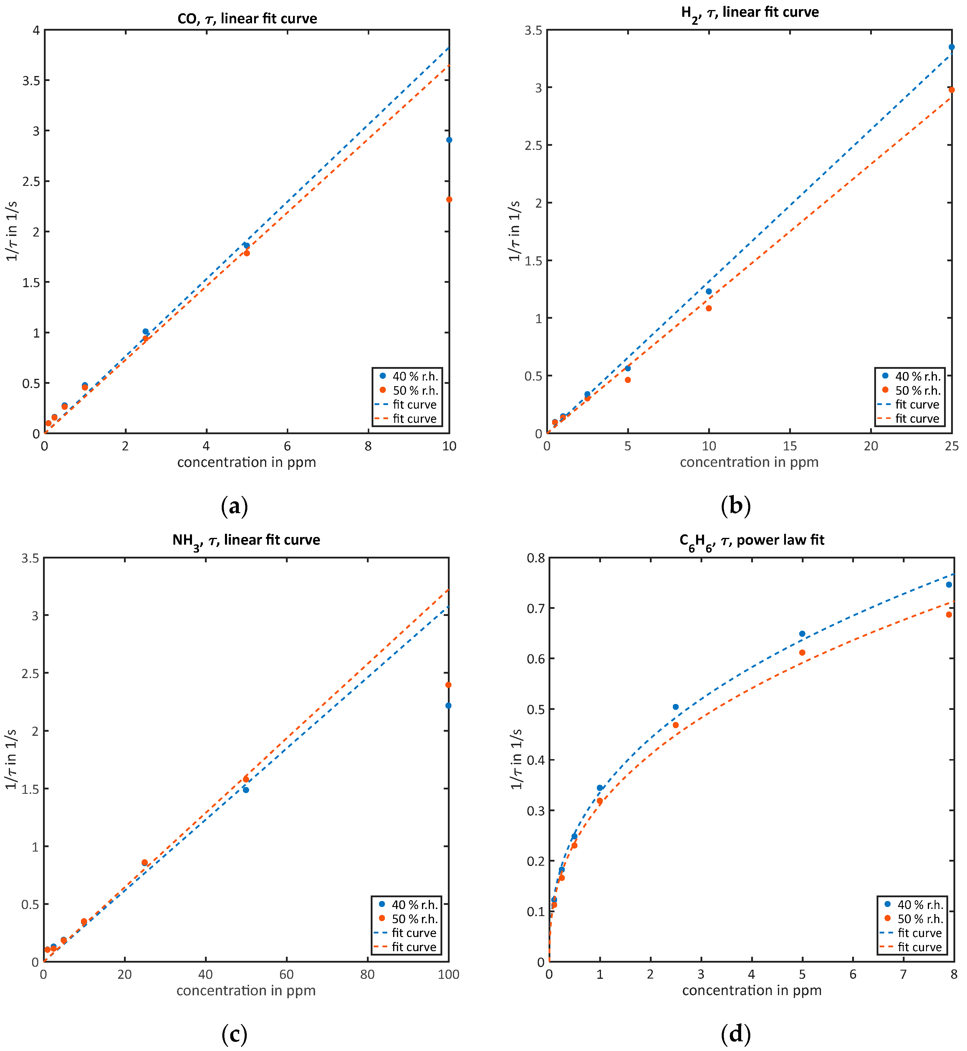
- For the quantification of high concentrations when the sensor almost reaches equilibrium surface coverage during the low-temperature phase, the time constant of the relaxation process is evaluated by taking the highest and lowest values of and evaluating the time-constant for reaching of the difference using the MATLAB function interp1:According to the solution of the simple differential Equation (3), the inverse value equals and is therefore linear to c. For practical reasons, the constant can be omitted as it is negligible in the high concentration range compared to . Therefore, the signal will be proportional to the gas concentration.
3. Results
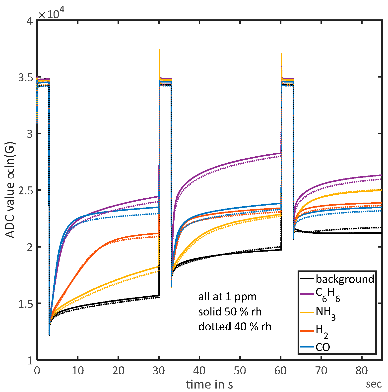
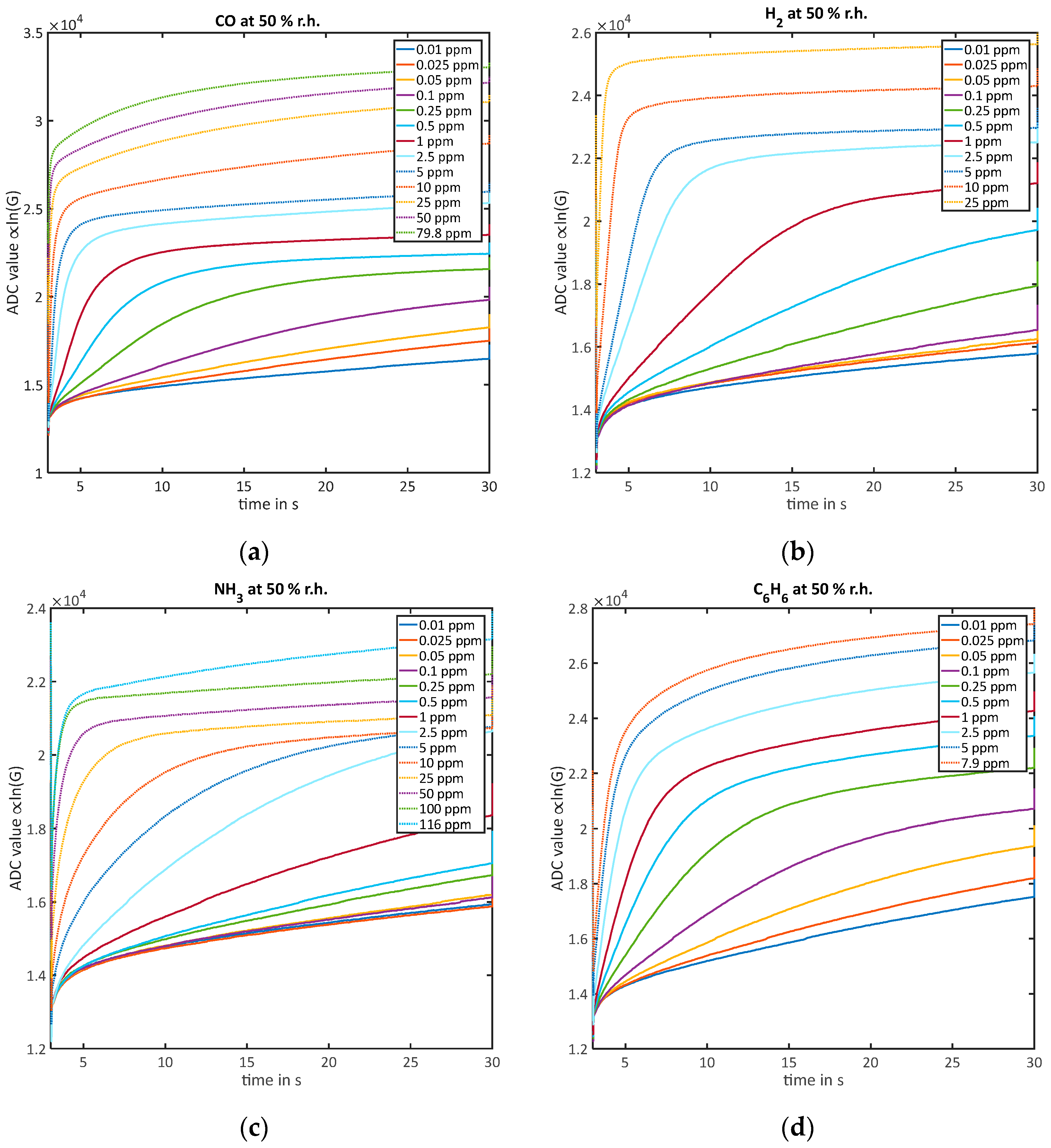
3.1. Overview
3.2. Quantification
3.2.1. Quantification of Low Concentrations without Reaching Equilibrium during the Low-Temperature Phase ()
3.2.2. Quantification of High Concentrations While Reaching Equilibrium during the Low-Temperature Phase ()
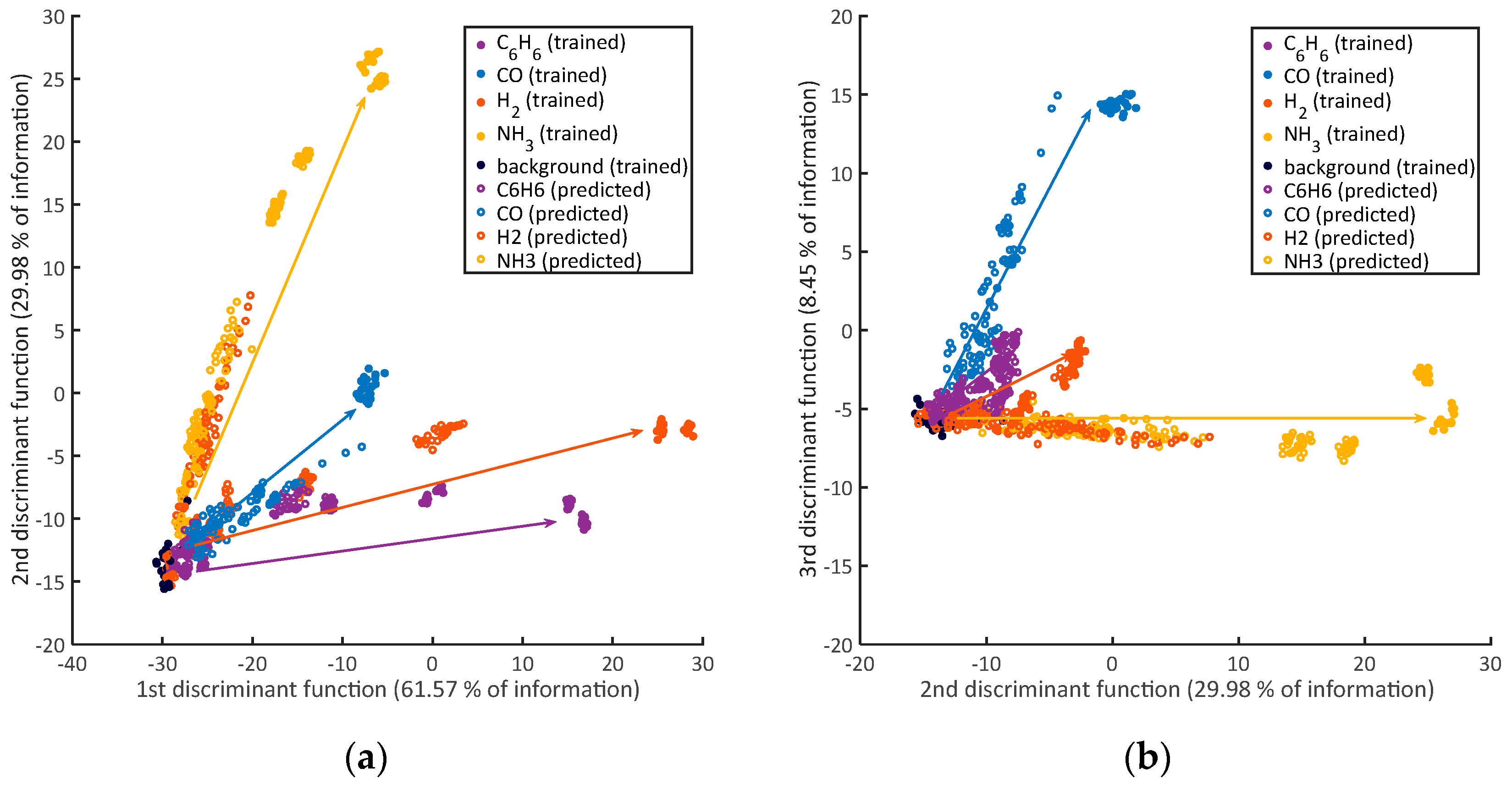
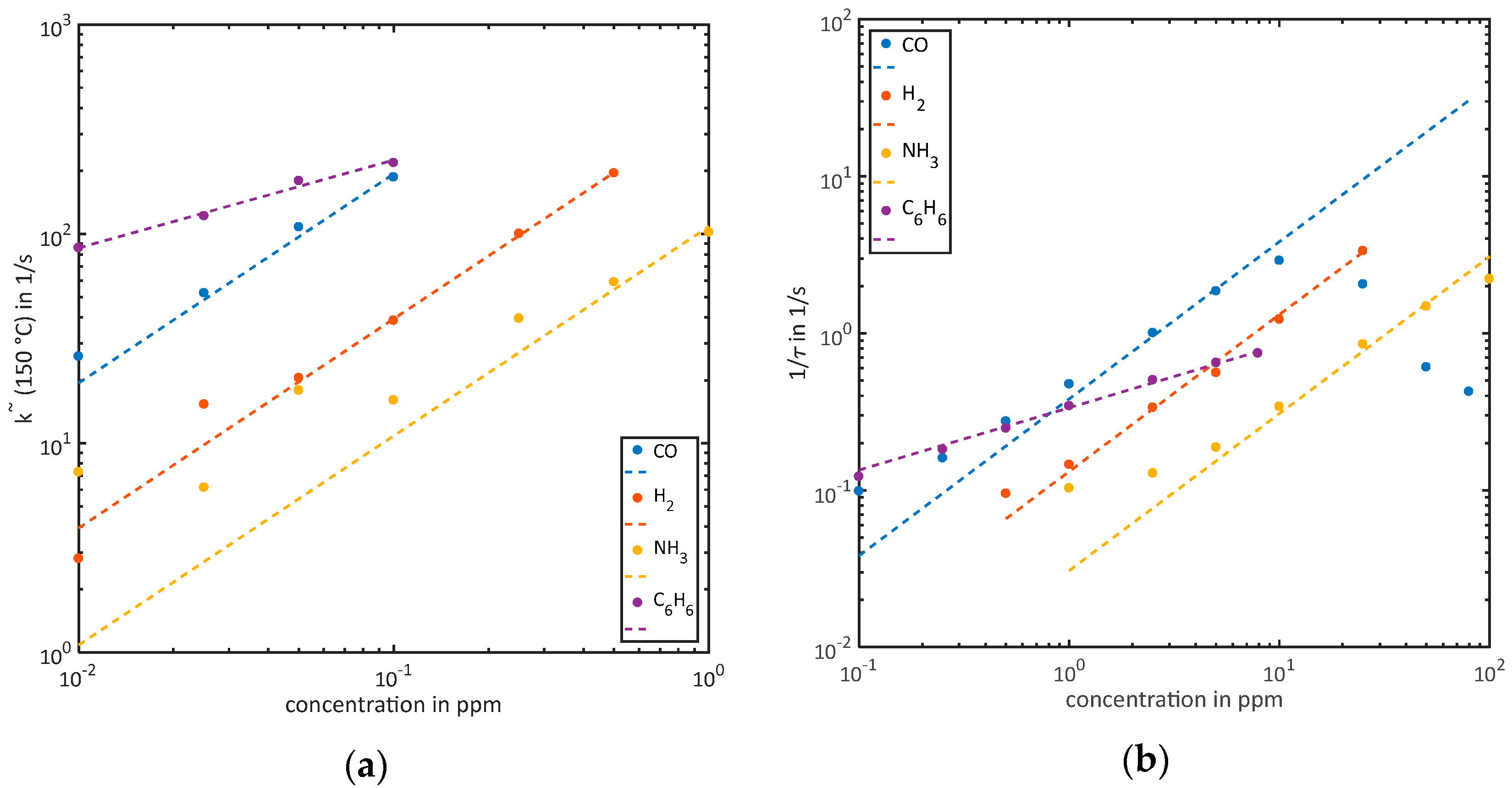
3.3. Identification
4. Discussion
5. Conclusions
Supplementary Materials
Author Contributions
Conflicts of Interest
References
- Kohl, D. Function and applications of gas sensors. J. Phys. D Appl. Phys. 2001, 34, R125. [Google Scholar] [CrossRef]
- De Angelis, L.; Riva, R. Selectivity and stability of a tin dioxide sensor for methane. Sens. Actuators B Chem. 1995, 28, 25–29. [Google Scholar] [CrossRef]
- Kohl, D.; Kelleter, J.; Petig, H. Detection of Fires by Gas Sensors. Sens. Update 2001, 9, 161–223. [Google Scholar] [CrossRef]
- Reimann, P.; Schütze, A. Fire detection in coal mines based on semiconductor gas sensors. Sens. Rev. 2012, 32, 47–58. [Google Scholar] [CrossRef]
- Maekawa, T.; Suzuki, K.; Takada, T. Odor identification using a SnO2-based sensor array. Sens. Actuators B 2001, 80, 3–6. [Google Scholar] [CrossRef]
- Peterson, P.; Aujla, A.; Grant, K.; Brundle, A.; Thompson, M.; Vande Hey, J.; Leigh, R. Practical Use of Metal Oxide Semiconductor Gas Sensors for Measuring Nitrogen Dioxide and Ozone in Urban Environments. Sensors 2017, 17, 1653. [Google Scholar] [CrossRef] [PubMed]
- Leidinger, M.; Sauerwald, T.; Reimringer, W.; Ventura, G.; Schütze, A. Selective detection of hazardous VOCs for indoor air quality applications using a virtual gas sensor array. J. Sens. Sens. Syst. 2014, 3, 253–263. [Google Scholar] [CrossRef]
- Llobet, E.; Brezmes, J.; Vilanova, X.; Sueiras, J.E.; Correig, X. Qualitative and quantitative analysis of volatile organic compounds using transient and steady-state responses of a thick-film tin oxide gas sensor array. Sens. Actuators B Chem. 1997, 41, 13–21. [Google Scholar] [CrossRef]
- Lee, A.P.; Reedy, B.J. Temperature modulation in semiconductor gas sensing. Sens. Actuators B Chem. 1999, 60, 35–42. [Google Scholar] [CrossRef]
- Gramm, A.; Schütze, A. High performance solvent vapor identification with a two sensor array using temperature cycling and pattern classification. Sens. Actuators B Chem. 2003, 95, 58–65. [Google Scholar] [CrossRef]
- Jurs, P.C.; Bakken, G.A.; McClelland, H.E. Computational methods for the analysis of chemical sensor array data from volatile analytes. Chem. Rev. 2000, 100, 2649–2678. [Google Scholar] [CrossRef] [PubMed]
- Eicker, H. Method and Apparatus for Determining the Concentration of One Gaseous Component in a Mixture of Gases. U.S. Patent 4012692A, 15 March 1977. [Google Scholar]
- Clifford, P.K.; Tuma, D.T. Characteristics of semiconductor gas sensors II. transient response to temperature change. Sens. Actuators 1982, 3, 255–281. [Google Scholar] [CrossRef]
- Ding, J.; Mcavoy, T.J.; Cavicchi, R.E.; Semancik, S. Surface state trapping models for SnO2-based microhotplate sensors. Sens. Actuators B Chem. 2001, 77, 597–613. [Google Scholar] [CrossRef]
- Nakata, S.; Ozaki, E.; Ojima, N. Gas sensing based on the dynamic nonlinear responses of a semiconductor gas sensor: Dependence on the range and frequency of a cyclic temperature change. Anal. Chim. Acta 1998, 361, 93–100. [Google Scholar] [CrossRef]
- Baur, T.; Schütze, A.; Sauerwald, T. Detektion von kurzen Gaspulsen für die Spurengasnalaytik. TM—Tech. Mess. 2017, 84, 88–92. [Google Scholar] [CrossRef]
- Schultealbert, C.; Baur, T.; Schütze, A.; Böttcher, S.; Sauerwald, T. A novel approach towards calibrated measurement of trace gases using metal oxide semiconductor sensors. Sens. Actuators B. Chem. 2017, 239, 390–396. [Google Scholar] [CrossRef]
- Barsan, N.; Weimar, U. Conduction Model of Metal Oxide Gas Sensors. J. Electroceram. 2001, 7, 143–167. [Google Scholar] [CrossRef]
- Yamazoe, N.; Shimanoe, K. Theory of power laws for semiconductor gas sensors. Sens. Actuators B Chem. 2008, 128, 566–573. [Google Scholar] [CrossRef]
- Bastuck, M.; Leidinger, M.; Sauerwald, T.; Schütze, A. Improved quantification of naphthalene using non-linear Partial Least Squares Regression. In Proceedings of the 16th International Symposium on Olfaction and Electronic Nose, Dijon, France, 28 June–1 July 2015; pp. 1–2. [Google Scholar]
- Wolfrum, E.J.; Meglen, R.M.; Peterson, D.; Sluiter, J. Metal oxide sensor arrays for the detection, differentiation, and quantification of volatile organic compounds at sub-parts-per-million concentration levels. Sens. Actuators B Chem. 2006, 115, 322–329. [Google Scholar] [CrossRef]
- Baur, T.; Schütze, A.; Sauerwald, T. Optimierung des temperaturzyklischen Betriebs von Halbleitergassensoren. Tech. Mess. 2015, 82, 187–195. [Google Scholar] [CrossRef]
- Madou, M.J.; Morrison, S.R. Chemical Sensing with Solid State Devices; Academic Press: San Diego, CA, USA, 1989; ISBN 0-12-464965-3. [Google Scholar]
- Barsan, N.; Schweizer-Berberich, M.; Göpel, W. Fundamental and practical aspects in the design of nanoscaled SnO2 gas sensors: A status report. Fresenius J. Anal. Chem. 1999, 365, 287–304. [Google Scholar] [CrossRef]
- Gurlo, A. Interplay between O2 and SnO2: Oxygen Ionosorption and Spectroscopic Evidence for Adsorbed Oxygen. ChemPhysChem 2006, 2041–2052. [Google Scholar] [CrossRef] [PubMed]
- Pulkkinen, U.; Rantala, T.T.; Rantala, T.S.; Lantto, V. Kinetic Monte Carlo simulation of oxygen exchange of SnO2 surface. J. Mol. Catal. A Chem. 2001, 166, 15–21. [Google Scholar] [CrossRef]
- Suematsu, K.; Yuasa, M.; Kida, T.; Yamazoe, N.; Shimanoe, K. Determination of Oxygen Adsorption Species on SnO2: Exact Analysis of Gas Sensing Properties Using a Sample Gas Pretreatment System. J. Electrochem. Soc. 2014, 161, B123–B128. [Google Scholar] [CrossRef]
- Yamazoe, N.; Suematsu, K.; Shimanoe, K. Extension of receptor function theory to include two types of adsorbed oxygen for oxide semiconductor gas sensors. Sens. Actuators B Chem. 2012, 163, 128–135. [Google Scholar] [CrossRef]
- Bastuck, M.; Baur, T.; Schütze, A. P7 Messunsicherheit und Funktionssicherheit von Messsystemen. In P7.3 - DAV3E: Data Analysis and Verification/Visualization/Validation Environment für die Multisensor-Datenfusion; 2016; pp. 729–734. Available online: http://www.ama-science.org/proceedings/details/2435 (accessed on 26 February 2018).
- Baur, T.; Schütze, A.; Sauerwald, T. Detection of short trace gas pulses. In Proceedings of the Sensor 2017, Nürnberg, Germany, 30 May–1 June 2017; pp. 87–91. [Google Scholar]
- Leidinger, M.; Schultealbert, C.; Neu, J.; Schütze, A.; Sauerwald, T. Characterization and calibration of gas sensor systems at ppb level—A versatile test gas generation system. Meas. Sci. Technol. 2018, 29. [Google Scholar] [CrossRef]
- Vaittinen, O.; Metsälä, M.; Persijn, S.; Vainio, M.; Halonen, L. Adsorption of ammonia on treated stainless steel and polymer surfaces. Appl. Phys. B 2014, 115, 185–196. [Google Scholar] [CrossRef]
- Gutierrez-Osuna, R. Pattern analysis for machine olfaction: A review. IEEE Sens. J. 2002, 2, 189–202. [Google Scholar] [CrossRef]
- Bârsan, N.; Hübner, M.; Weimar, U. Conduction mechanisms in SnO2 based polycrystalline thick film gas sensors exposed to CO and H2 in different oxygen backgrounds. Sens. Actuators B Chem. 2011, 157, 510–517. [Google Scholar] [CrossRef]
- Kamp, B.; Merkle, R.Ã.; Lauck, R.; Maier, J. Chemical diffusion of oxygen in tin dioxide: Effects of dopants and oxygen partial pressure. 2005, 178, 3027–3039. [Google Scholar] [CrossRef]
- Danzer, K.; Currie, L.A. Guidelines for calibration in analytical chemistry. Part I. Fundamentals and single component calibration (IUPAC Recommendations 1998). Pure Appl. Chem. 1998, 70, 993–1014. [Google Scholar] [CrossRef]


| Gas | Concentrations Measured | -Evaluation | -Evaluation |
|---|---|---|---|
| CO | 0.01–79.8 ppm | 0.01–0.1 ppm | 0.1–5 ppm |
| H2 | 0.01–25 ppm | 0.01–0.5 ppm | 0.5–25 ppm |
| NH3 | 0.01–116 ppm | 0.01–1 ppm | 1–50 ppm |
| C6H6 | 0.01–7.9 ppm | 0.01–0.1 ppm | 0.1–7.9 ppm |
| Gas | Humidity | Fit Function | |||
|---|---|---|---|---|---|
| CO | 40%RH | 1939 | - | 0.9851 | |
| - | 50%RH | - | 1995 | - | 0.9252 |
| H2 | 40%RH | 393.1 | - | 0.9986 | |
| - | 50%RH | - | 351.9 | - | 0.9983 |
| NH3 | 40%RH | 108.5 | - | 0.9381 | |
| - | 50%RH | - | 108.9 | - | 0.9606 |
| C6H6 | 40%RH | 569.9 | 0.4065 | 0.9835 | |
| - | 50%RH | - | 691.1 | 0.4935 | 0.9938 |
| Gas | Humidity | Fit Function | |||
|---|---|---|---|---|---|
| CO | 40%RH | 0.3827 | - | 0.9874 | |
| - | 50%RH | - | 0.365 | - | 0.9883 |
| H2 | 40%RH | 0.1317 | - | 0.9972 | |
| - | 50%RH | - | 0.1167 | - | 0.9955 |
| NH3 | 40%RH | 0.03078 | - | 0.9888 | |
| - | 50%RH | - | 0.03224 | - | 0.9960 |
| C6H6 | 40%RH | 0.3358 | 0.3977 | 0.9963 | |
| - | 50%RH | - | 0.3114 | 0.3987 | 0.9942 |
© 2018 by the authors. Licensee MDPI, Basel, Switzerland. This article is an open access article distributed under the terms and conditions of the Creative Commons Attribution (CC BY) license (http://creativecommons.org/licenses/by/4.0/).
Share and Cite
Schultealbert, C.; Baur, T.; Schütze, A.; Sauerwald, T. Facile Quantification and Identification Techniques for Reducing Gases over a Wide Concentration Range Using a MOS Sensor in Temperature-Cycled Operation. Sensors 2018, 18, 744. https://doi.org/10.3390/s18030744
Schultealbert C, Baur T, Schütze A, Sauerwald T. Facile Quantification and Identification Techniques for Reducing Gases over a Wide Concentration Range Using a MOS Sensor in Temperature-Cycled Operation. Sensors. 2018; 18(3):744. https://doi.org/10.3390/s18030744
Chicago/Turabian StyleSchultealbert, Caroline, Tobias Baur, Andreas Schütze, and Tilman Sauerwald. 2018. "Facile Quantification and Identification Techniques for Reducing Gases over a Wide Concentration Range Using a MOS Sensor in Temperature-Cycled Operation" Sensors 18, no. 3: 744. https://doi.org/10.3390/s18030744