External Second Gate, Fourier Transform Ion Mobility Spectrometry: Parametric Optimization for Detection of Weapons of Mass Destruction

Sandia National Laboratories, Analytical Materials Sciences Department, P.O. Box 969, Mail Stop 9403, Livermore, CA 94551-0969, USA
Sensors 2004, 4(1), 1-13; https://doi.org/10.3390/s40100001
Submission received: 2 May 2003
/
Accepted: 11 March 2004
/
Published: 30 March 2004
Abstract
:Ion mobility spectrometry (IMS) is recognized as one of the most sensitive and robust techniques for the detection of narcotics, explosives and chemical warfare agents. IMS is widely used in forensic, military and security applications. Increasing threat of terrorist attacks, the proliferation of narcotics, Chemical Weapons Convention (CWC) treaty verification as well as humanitarian de-mining efforts have mandated that equal importance be placed on the time required to obtain results as well as the quality of the analytical data. [1] In this regard IMS is virtually unrivaled when both speed of response and sensitivity have to be considered. [2] The problem with conventional (signal averaging) IMS systems is the fixed duty cycle of the entrance gate that restricts to less than 1%, the number of available ions contributing to the measured signal. Furthermore, the signal averaging process incorporates scan-to-scan variations that degrade the spectral resolution contributing to misidentifications and false positives. With external second gate, Fourier Transform ion mobility spectrometry (FT-IMS) the entrance gate frequency is variable and can be altered in conjunction with other data acquisition parameters (scan time and sampling rate) to increase the spectral resolution to reduce false alarms and improve the sensitivity for early warning and contamination avoidance. In addition, with FT-IMS the entrance gate operates with a 50% duty cycle and so affords a seven-fold increase in sensitivity. Recent data on high explosives are presented to demonstrate the parametric optimization in sensitivity and resolution of our system.
Ion Mobility Spectrometry
Ion mobility spectrometry (IMS) is based on the atmospheric pressure ionization of sample vapors and the subsequent separation of individual components of the sample mixture as they transit an electric field gradient against a neutral counter-flowing gas stream. The sample vapors are drawn into the detector, and ionized through proton transfer or electron capture reactions (depending on the polarity of electric field) to form “product ions”. The ions are periodically pulsed into the separation region of the spectrometer by an electronic gating grid where they are accelerated by an electric field gradient and differentiated according to their velocities against the counter-flowing drift gas. The separation region begins at the gating grid and terminates at a collecting electrode. The spectrum of ion arrival times at the collecting electrode indicates the relative mobility of each ion through the separation region. The individual ion mobility's are determined by the mass, charge and collisional cross-section of the ions as well as the number density of the opposing drift gas molecules. To a first approximation, the number of collisions each sample ion experiences with the opposing drift gas molecules determines the differences in ion mobility. For example, ions having the same charge but experiencing a greater number of collisions will have greater differences in ion mobility. Thus, a better separation of the sample mixture will result. Differences in collision frequency may be caused by differences cross sectional area and/or ionic mass as well as ionic charge. Response in IMS is measured as a function of ion current produced versus the ion arrival time at the collecting electrode after each 20-25 ms analytical cycle. Compound identification is based on comparison of the ion arrival time or “ion mobility spectrum” generated from the sample with the spectrum of a known standard. In typical IMS instruments spectra are obtained by pulsing open the electronic gating grid (entrance gate) of the time-of-flight drift tube (separation region) for 0.2 ms to admit an ion pulse. This brief 0.2 ms entrance gate pulse represents ≤1% of the total 20-25 ms analytical, “duty cycle” of the instrument. With conventional IMS more than 99% of the ions formed are discarded and never reach the detector as a result of the 1% duty cycle of the entrance gate [3]. With sample concentrations at the part-per-billion to part-per-trillion level or initial sample quantities in the picogram to femtogram range, such losses can be catastrophic to detection and identification. Increasing the temporal width of the gate opening pulse would admit more ions and increase the signal strength, however, a short duration pulse is necessary to minimize ion diffusion and subsequent peak broadening which results in decreased spectral resolution. Therefore, to achieve an acceptable signal-to-noise ratio (S/N) with such a low duty cycle, multiple scans are taken and summed with a computer. This summation or “signal averaging” process introduces an additional source of peak broadening in conventional IMS. The consequence of this trade off between sensitivity and resolution has resulted in the relatively poor resolution typical of all conventional IMS instruments. Furthermore, false positives resulting from peak misidentification can endanger first response personnel, cost millions of dollars in emergency services and cause unnecessary psychological harm to the general population.
Fourier Transform Ion Mobility Spectrometry
An alternative method of signal acquisition based on ion mobility spectrometry utilizes a two-gate design and involves the Fourier transformation of a frequency domain ion mobility interferogram to recover the normal time domain ion mobility spectrum [4]. The interferogram is generated as the ions pulsed into the spectrometer by the entrance gate interact with a second simultaneously pulsed “exit” gate. The ions reach the second gate after the time-of-flight delay for ion transit through the separation region. As a consequence of this delay time, the pulsing ion stream comes into and out of phase with the second gate as it opens and closes. An interference signal is produced that rises and falls depending on the degree to which the second gate is opened or is closing. For an ion to have maximum contribution to the signal it must be traveling at a velocity such that its arrival just matches the gate opening frequency of the second gate. Minimal signal contribution is made if the ion reaches the gate as it closes. For a mixed sample containing a broad range of ion velocities there must be a broad range of gate opening frequencies to record the signal for each of the ion velocities. This is accomplished by pulsing open the gates with a square wave at continually increasing frequency from a few Hertz up to tens of kilo-Hertz over the analytical cycle. In addition, since the waveform is square, the gates are open for the same amount of time they are closed as they increase in frequency over the entire analytical cycle. All of the velocity information about each of the ions sampled is encoded in the interference signal (the interferogram). The mathematical relationship between the ions velocity and the gate frequency allows for the Fourier transformation of the frequency interferogram and the recovery of the time domain ion mobility spectrum. In the mid nineteen eighties the earliest FT-IMS designs by Hill, et al. [4], had the two electronic gating grids located inside the drift tube with each gate synchronously pulsed opened 50% of the time as described above. Half of the initial ion population approaching the first gate would be admitted into the drift tube (separation region) and of this population only half would pass through the second gate to contribute to the signal. With this design, a net 25% duty cycle was achieved and the S/N improved by a factor of five (√25).
External Second Gate, Fourier Transform Ion Mobility Spectrometry
In our Sandia design, we have eliminated the internal second gate and developed a FT-IMS system capable of achieving a 50% duty cycle and higher resolution than conventional IMS [5, 6], see Figures 1-2. By modifying a single gate, signal-averaging instrument (Barringer Ion Scan 400, Barringer Instruments, New Providence NJ), we have configured a two-gate FT-IMS instrument design in which the function of the second, internal hardware gate is performed externally, outside of the drift tube, in the electronics. Without the loss of ion transmission at the second hardware gate we have been able to achieve a seven fold signal-to-noise enhancement (S/N = √50). Of particular importance is the improved resolving power afforded by the external second gate, FT-IMS method. By increasing the high-end scanning frequency up to 40 kilo Hertz we have improved the spectral resolution compared to conventional IMS systems [6]. The broad asymmetric peaks observed with IMS are due to clustering, recombination and various ion-molecule reactions occurring in the drift tube during time-of-flight, which alter the velocities of ions, see Figures 1a, 2, 3, 4, 5 and 6a. While these variations are all recorded in the final IMS spectrum that represents the averaged signal, they are eliminated with the FT-IMS technique. Only ions of constant velocity contribute to the measured signal. This occurs because the FT-IMS mode needs a constant frequency difference between the ion stream “beat” against the second gate to generate a constant beat frequency. Ions that react during their transit of the drift space alter their velocities and have no well-defined drift time. These ill-defined ions produce random incoherent signals at the second gate, adding only to the DC signal level and background noise. Signal-averaging instruments, on the other hand, incorporate the spectral broadening due to this phenomenon in the final signal output. We have demonstrated improved resolution and increased signal-to-noise compared to both the single gate signal-averaging IMS and the internal, two-gate FT-IMS designs. The electronic and software modifications we have developed enable us to adapt all common single-gate, signal-averaging IMS instruments to this external second gate FT-IMS method
FT-IMS Theory
A two-gate ion mobility spectrometer [4] designed to operate in the Fourier Transform mode requires the following four features. (1) A gating signal generator which produces a binary (on, off) square wave. (2) The entrance and exit gates are always driven simultaneously by the same square wave, with zero phase delay. (3) The scanning parameter is the square wave frequency. (4) The FT-IMS interferogram generated is recorded with a computer, which also performs Fourier transformation of the data to recover the normal ion mobility spectrum.
In the operation of a two-gate Fourier Transform spectrometer, a particular gate timing sequence is repeated many times, before the scanning parameter is changed. The time constant of the amplifier is too long to follow individual ion pulses or high frequency noise. Therefore the signal output represents the time averaged dc ion current at the present value of the scanning parameter. In addition, the gates themselves act as filters for the ions streaming through the drift tube. Depending on the characteristic transit times of the ions present and the gate timing sequence, some ions will reach the detector with maximum intensity, some with intermediate intensity and some not at all. The filtering action of the gates and the time averaged signal output may be represented by a gate correlation function.
That is, the intensity of ions with transit time t, m(t), is multiplied by the fraction of these ions that reach the detector and summed over all transit times to yield the detector signal. The gate function has a characteristic periodicity (frequency ν, period τ = ν−1) and a phase delay (Δt). In an FT scan the phase delay is held at zero while the frequency is swept. Scanning over a range of frequencies generates a family of gate correlation functions. The gate correlation functions, ε(τ, ν) are autocorrelation functions representing the filtering action of the gates as a function of frequency. The maximum value of ε(τ, ν) is 0.5; the fractional time the entrance gate is open.
The placement of the second gate also determines the collection efficiency by affecting ion transmission to the collector. If the second ion gate were to be physically placed inside of the drift tube just ahead of the collector and beat against the streaming ions to generate the interferogram it would reduce the ion transmission to the collector since it, like the entrance gate is only open for 50% of the time. The net effective duty cycle would then be reduced to 25% [4]. However it is possible to perform the function of the second gate outside of the drift tube in the electronics with a simulated, external second gate. The advantages of this technique are retention of the 50% duty cycle, maximum signal-to-noise enhancement, and the ease of adapting this method to existing commercially available single gate instruments
Experimental
All analyses were performed on a Barringer Ion Scan Model 400 (Barringer Instruments, New Providence, New Jersey) operated in the explosives (negative ion) detection mode. The high voltage was set at −2000V. The drift tube temperature was 105 oC, pressure 101.7 kPa, inlet temperature 240 oC, desorber temperature 225 oC, drift flow 350 mL/min, sample flow 300 mL/min. Explosive samples (Radian Corporation, USA) were dissolved as received in reagent grade acetone (Fischer Scientific, USA). The explosive solutions were deposited by syringe on the manufacturers' glass fiber sample cartridges. The acetone was allowed to evaporate and the cartridges inserted into the spectrometer.
Results and Discussion
The operator controlled instrumental parameters affecting sensitivity and resolution in external second gate, Fourier transform ion mobility spectrometry (FT-IMS) are: (1) The frequency range selected for the linearly ramped square wave. (2) The number of number of data points/second sampled. (3) The resulting speed of the frequency sweep. Ideally, the speed of the data acquisition system should be maximized to take as much data as fast as possible in order to be able to track short-lived transient species in the detector. This is particularly true with miniaturized IMS drift tubes where transit times are very brief.
Figure 1 compares the spectra of the reactant ion (left) generated by ionization of the drift gas and the calibrant ion (right) used for peak reference and identification at various frequency range settings. Figure 1a displays the peaks resulting from operation of the IMS instrument in the conventional signal-averaging mode. Figures 1b, 1c, and 1d show the same two peaks generated on the same instrument in the FT-IMS mode. In each case the number of data and the sampling rate are 65,536 and 65,536 points/second resulting in one second scan times. The only variable is the frequency range selected. The peak intensity is highest (92 for FT-IMS versus 6.5 for IMS) when the scanning frequency is 10 kHz, while the resolving power is greatest at 40 kHz. The increase in resolving power with frequency range swept can be traced by monitoring the small shoulder on the predominant reactant ion peak in figure 1b. As the frequency is increased to 20 kHz, and then to 40 kHz, the shoulder is clearly separated from the major peak. The higher frequency FT-IMS scans monitor increasingly smaller temporal slices of the ion pulse resulting in decreasing signal intensity: 52 at 20 kHz and 27 at 40 kHz, respectively.
Figure 2 displays the spectra generated from a 100 ppb solution of TNT in acetone deposited onto a sample cartridge and inserted into the IMS after the acetone was evaporated. The signal-averaged IMS spectrum in Figure 2a is shown on the same scale as the most intense FT-IMS spectrum (1.0 second, 1.0 kHz) in Figure 2b for the same sample. The total data acquisition time for the signal-averaged IMS spectra was 6.0 seconds where the total acquisition time for the FT-IMS spectra shown in 2b was three seconds. As the scan time is reduced to 0.5 seconds at 10 kHz and to 0.25 seconds at 20 kHz the resulting peak intensity decreases with increasing scan speed at these settings.
The spectral information lost beyond 15 ms in Figure 2d (the 0.25 second, 20 kHz scan) was found to be due to the low pass cut off filtering used for this particular analysis. The total data acquisition times for Figures 2c and 2d were 1.5 seconds (3 scans) and 2.5 seconds (10 scans), respectively. All three of the FT-IMS spectra were generated at a sampling rate of 65,536 data points/second
Figure 3 compares the spectra resulting from identical samples of the explosive PETN as a function of parametric settings. Figures 3a (6.0 second acquisition) and 3b (3.0 second acquisition) again demonstrate the striking increase in signal-to-noise achieved using the FT-IMS method. It should be noted that all of the spectra were generated in real time following manual sample insertion. Therefore they are difficult to reproduce from run to run. The mixture of ionic species formed in the ionization region of the detector has disparate vapor pressures and the spectral signature may change from run-to-run over the course of the analysis. The spectra selected however, display many of the same prominent peaks and are representative of the relative intensity and spectral complexity at various instrumental settings. Figure 3b and 3c again demonstrate the relative effect of scanning frequency. Figure 3d shows the recovered spectral information at around 15 ms that had been eliminated by the low pass cut-off filter used in the last example (Figure 2d).
Figure 4 shows the effect of scan time at various frequencies for the explosive HNS.
The number of data points divided by the sampling rate (data points/second) determines the analysis time for each, individual frequency ramped scan. As the scan time is decreased so is the relative peak intensity at each setting. Figure 4a shows the spectra generated by signal-averaging IMS while Figure 4b, 4c (each at 10 kHz) and 4d show the effect of scan time at the highest sampling rate used for this set of experiments, 65,536 data points/second. However, a 20 kHz frequency range was required to scan in 0.25 seconds at this sampling rate (65,536 data points/second) as shown in Figure 4d. Data for this sample at 40 kHz and 0.25 seconds scan time resulted in significant loss in signal-to-noise and is not shown
Figure 5 displays the IMS spectrum of the explosive HMX along with the 10 kHz, 20 kHz, and 40 kHz FT-IMS spectra of the explosive scanned at 1.0, 0.5 and 0.25 seconds, respectively. The signal-averaged spectrum in 5a is comparable in intensity and features to the 40 kHz FT-IMS spectra in 5d, however 5a is a 6.0 second acquisition while 5d required 3.0 seconds.
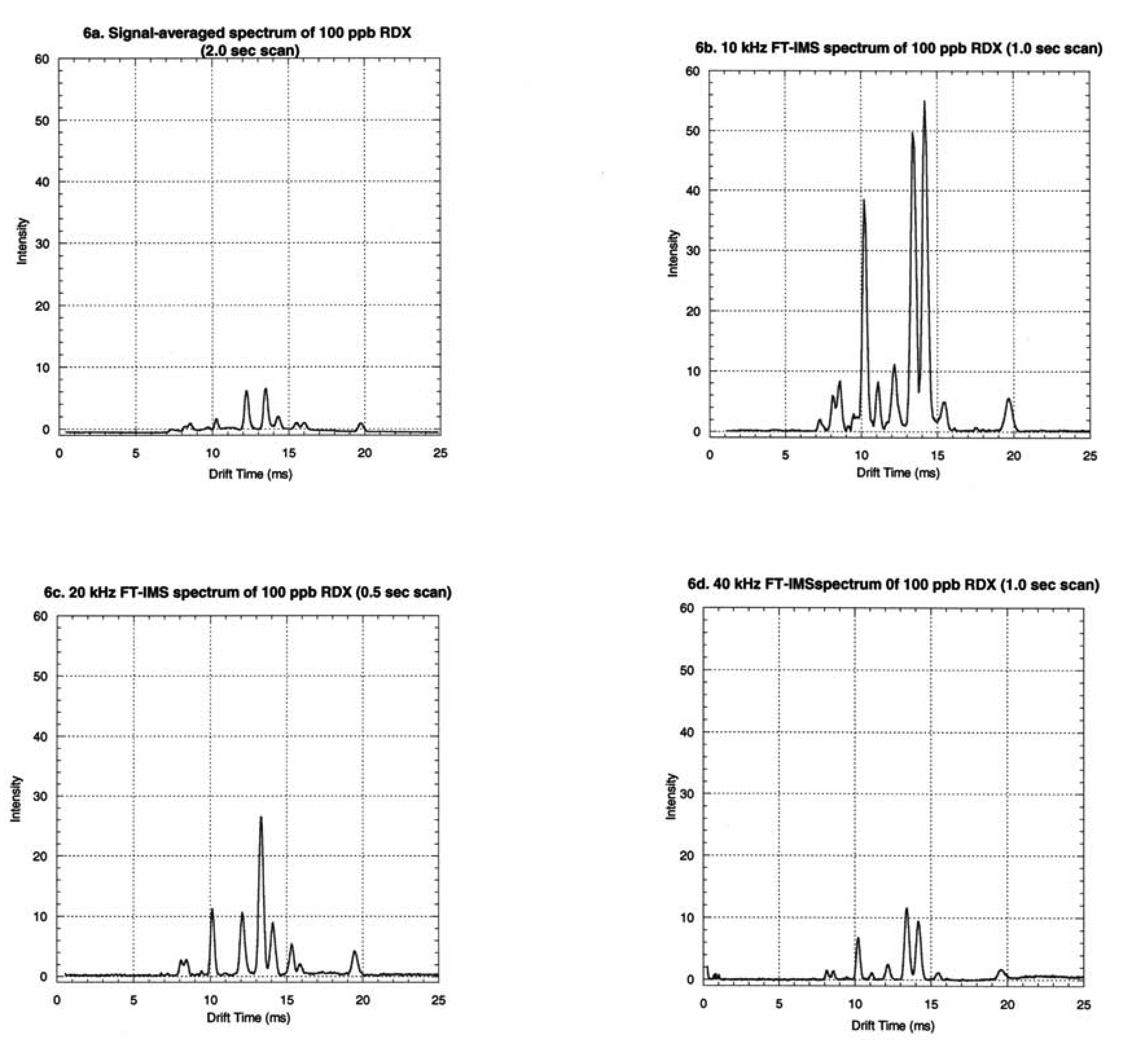
Figure 6 compares the spectra generated by the two methods from a sample of RDX. Figure 6a shows the response resulting from 2.0 seconds total acquisition in the conventional signal-averaging mode. Acquisition times of 3.0 and 6.0 seconds in this mode did not result in significant differences in spectral intensity or features. Figure 6b displays the significant advantage in chemical identification capability achieved by enabling the signature peaks to be monitored well above the baseline noise. The RDX was monitored at the maximum sampling rate using 1.0 seconds scans over a 10 kHz frequency range. The total acquisition time was 3.0 seconds. Figure 6c and 6d display the RDX spectra produced by 20 kHz and 40 kHz scans over a total acquisition time of 3.0 seconds. Once again the 40 kHz scan, while producing a somewhat larger response, is similar in peak intensity to that of the signal averaged spectrum.
Peak broadening in IMS is primarily determined by the temporal width of the entrance gate pulse (typically about 0.2 ms), electric field in-homogeneity, Coulombic repulsion between ions, and diffusional broadening as the ions transit the drift space [7]. Other contributors to peak broadening include ion-molecule reactions that can occur during time-of-flight and the process of averaging multiple spectra. Resolution in IMS is traditionally calculated as defined by Equation (1) below:
where td is the drift time and w is the full width at half maximum (in drift time units) for the peak. This calculation is drift time dependent and also ignores peak asymmetry below half-maximum. As a result broad peaks with long drift times or peaks that exhibit tailing below half maximum are ascribed misleading resolution values. A more uniform way of describing peak quality is peak aspect ratio, or the ratio of the peak height to the width at the base where: AR = h/wb, Equation 2. The taller and more narrow a peak (i.e., high aspect ratio), the easier it is to resolve it from a neighboring peak. FT-IMS can routinely produce peaks with aspect ratios up to 20 times larger than signal averaging IMS (see Figure 1a) by selecting high sensitivity parametric settings. In situations where sample introduction is consistent, as with industrial processes where formulations are constant, FT-IMS affords the ability to tune the resolving power (Figure 1b-d) to suit the needs of the separation problem. The combined features of higher sensitivity, resolution, peak aspect ratio, and ease of adaptability to conventional IMS drift tubes and ionization sources has made FT-IMS the solution to the traditional limitations of signal-averaging IMS. Table 1, below compares the resolution as calculated by Equation 1 with the peak aspect ratio.
Ion mobility is measured by determining the time it takes for the ion to transit the separation region of the drift tube. Because the ion mobility depends on instrumental design and the number density of the neutral drift gas, reduced mobilities (Ko) at Standard Temperature and Pressure are reported to identify the ions. The peaks compared in Table 1 have drift times of 10.3 and 12.2 ms and are listed by their reduced mobility constants 1.84 and 1.54 respectively, as calculated below by Equation 3, below:
Where: V is the voltage drop across the drift tube, L is the drift length in cm, td is the drift time in sec, P is the drift gas pressure in Torr, and T is the Temperature.
Conclusion
Fourier transform ion mobility spectrometry (FT-IMS) has several advantages over conventional ion mobility spectrometers. First, the effective percentage of the analytical cycle time wherein sample ions are admitted into the spectrometer is much greater. The result is significantly improved signal-to-noise. Second, the phasing action of the two-gate Fourier transform method eliminates the peak tailing due to variations in ion velocities attributed to random ion-molecule reactions occurring in the time-of-flight drift tube. Third, information about all ion velocities is obtained simultaneously, eliminating the need to average over many analytical cycles. With our External Second Gate FT-IMS the function of the second ion gate is emulated in the electronics and as such eliminates the need for a physical ion gate placed inside of the drift tube. The result is that we have further increased the effective duty cycle relative to conventional signal-averaging ion mobility spectrometers.
The sensitivity achievable in convention signal-averaging IMS is routinely in the low part-per-billion range making the technique attractive for a wide range of security and forensic applications. With conventional IMS peak detection thresholds must be set nearer the instrumental detection limit so as not to overlook any potentially valuable information. Once the operator is forced into peak detection thresholds on the same order of magnitude as trace interferences, unambiguous peak identification becomes very difficult. This may result in costly (or deadly) false alarms, particularly when complex sample matrices are introduced into the detector. As a result, the ability to cleanly separate closely spaced peaks is critical.
Resolution has always been moderate to poor with conventional IMS instruments. This performance limitation has traditionally been tolerated due to the profound sensitivity of the technique, the real-time response and the ability to operate at atmospheric pressure (no vacuum pumps required). The resolution problem has also prevented miniaturization of the instrument. In other words, can a smaller instrument be expected to perform as well as the full size equivalent? Usually the answer is no. However, FT-IMS affords the greatest opportunity to achieve this goal. The inherent advantage of FT-IMS compared to conventional IMS systems is the ability to collect 50 times more ions to contribute to the signal (signal-to-noise increase = square root of 50 or about 7) and the improved resolving power afforded by the filtering action of the dual gate design.
This is a critical performance advantage on the scale of miniaturized spectrometer hardware where drift lengths are shorter and ion throughput is much smaller.
References and Notes
- Erickson, B. Anal. Chem. 1998, 70, 397–400A.
- Corriveau, J. In: Analytical methods for Environmental Sampling of Chemical Warfare Agents and their Degradation Products; Watson, A.P., Kistner, S., Eds.; 1994; pp. 147–488. [Google Scholar]
- U.S. Congress. Office of Technology Assessment; Technology Against Terrorism: The Federal Effort, 1991; pp. 84–86. [Google Scholar]
- Knorr, F.J.; Eatherton, R.L.; Siems, W.F.; Hill, H.H. Anal. Chem. 1985, 57, 402–406.
- Tarver, E.E.; Stamps, J.; Jennings, R.; Siems, W.F. Int. J. Ion Mobility Spectr. 2001, 4(1), 57–59.
- Tarver, E.E.; Stamps, J.; Jennings, R. Proceedings: 7th International Symposium on the Analysis and Detection of Explosives, June 25 2001; Edinburgh, Scotland.
- Siems, W.F.; Ching, Wu; Hill, H.H.; Tarver, E.E. Anal. Chem. 1994, 66, 4195–4201.
- Ching, Wu; Siems, W.F.; Asbury, G.R.; Hill, H.H. Anal. Chem. 1998, 70(23), 4929–4938.
Figure 1.
Background Spectra displaying the reactant ion (left) and calibrant ion (right) peaks. 1a. Signal averaged IMS spectrum. 1b. Fourier transform IMS spectra at 10 kHz. 1c. Fourier transform spectrum at 20 kHz. 1d. 40 kHz ending frequency.
Figure 1.
Background Spectra displaying the reactant ion (left) and calibrant ion (right) peaks. 1a. Signal averaged IMS spectrum. 1b. Fourier transform IMS spectra at 10 kHz. 1c. Fourier transform spectrum at 20 kHz. 1d. 40 kHz ending frequency.

Figure 2.
Spectra produced by 100 ppb solution of TNT (acetone evaporated). 2a. Signal averaged IMS spectrum (6 sec scan). 2b. 10 kHz FT-IMS spectrum (1.0 sec scan). 2c. 10 kHz FT-IMS spectrum (3;0.5 sec scan) 2d. 20 kHz FT-IMS spectrum (10;0.25 sec scan).
Figure 2.
Spectra produced by 100 ppb solution of TNT (acetone evaporated). 2a. Signal averaged IMS spectrum (6 sec scan). 2b. 10 kHz FT-IMS spectrum (1.0 sec scan). 2c. 10 kHz FT-IMS spectrum (3;0.5 sec scan) 2d. 20 kHz FT-IMS spectrum (10;0.25 sec scan).

Figure 3.
Spectra produced by 100 ppb solution of PETN monitored by fixed frequency, signal averaging and three linearly ramped gating frequencies. 3a. Signal averaged response (6.0 sec scan). 3b.10 kHz FT-IMS. (3;1.0 sec scan) 3c. 20 Khz FT-IMS. (0.5 sec scan) 3d. 40 kHz FT-IMS (1.0 sec scan).
Figure 3.
Spectra produced by 100 ppb solution of PETN monitored by fixed frequency, signal averaging and three linearly ramped gating frequencies. 3a. Signal averaged response (6.0 sec scan). 3b.10 kHz FT-IMS. (3;1.0 sec scan) 3c. 20 Khz FT-IMS. (0.5 sec scan) 3d. 40 kHz FT-IMS (1.0 sec scan).

Figure 4.
Spectra produced by 100 ppb solution of HNS (acetone evaporated). 4a. Signal averaged IMS spectrum (3.0 sec scan). 4b. FT-IMS spectrum generated by 1.0 sec scan at 10 kHz. 4c. FT-IMS spectrum generated by 0.5 sec scan at 10 kHz. 4d. FT-IMS spectrum generated by 0.25 sec scan at 20 kHz.
Figure 4.
Spectra produced by 100 ppb solution of HNS (acetone evaporated). 4a. Signal averaged IMS spectrum (3.0 sec scan). 4b. FT-IMS spectrum generated by 1.0 sec scan at 10 kHz. 4c. FT-IMS spectrum generated by 0.5 sec scan at 10 kHz. 4d. FT-IMS spectrum generated by 0.25 sec scan at 20 kHz.

Figure 5.
Spectra produced by 100 ppb solution of HMX at variable frequency. 5a. Signal averaged spectrum, 6.0 sec acquisition. 5b. 10 kHz FT-IMS spectrum, 1.0 sec scan. 5c. 20 kHz FT-IMS spectrum, 0.5 sec scan. 5d. 40 kHz FT-IMS spectrum, 0.25 sec scan.
Figure 5.
Spectra produced by 100 ppb solution of HMX at variable frequency. 5a. Signal averaged spectrum, 6.0 sec acquisition. 5b. 10 kHz FT-IMS spectrum, 1.0 sec scan. 5c. 20 kHz FT-IMS spectrum, 0.5 sec scan. 5d. 40 kHz FT-IMS spectrum, 0.25 sec scan.

Figure 6.
Spectra produced by 100 ppb solution of RDX. 6a. Signal averaged IMS spectrum (2.0 sec acquisition). 6b. 10 kHz FT-IMS spectrum, 1.0 sec scan. 6c. 20 kHz FT-IMS spectrum, 0.5 sec scan. 6d. 40 kHz FT-IMS spectrum, 1.0 sec scan.
Figure 6.
Spectra produced by 100 ppb solution of RDX. 6a. Signal averaged IMS spectrum (2.0 sec acquisition). 6b. 10 kHz FT-IMS spectrum, 1.0 sec scan. 6c. 20 kHz FT-IMS spectrum, 0.5 sec scan. 6d. 40 kHz FT-IMS spectrum, 1.0 sec scan.


| Peak Resolution (Ko =1.84, 10.3 ms drift time) | Peak Aspect Ratio (Ko =1.84) | |||||||
|---|---|---|---|---|---|---|---|---|
| (IMS) | (Fourier Transform-IMS) | (IMS) | (Fourier Transform-IMS) | |||||
| Spectrum: | a | b | c | d | a | b | c | d |
| Figure 2: TNT | 40.97 | 30.27 | 29.42 | 36.59 | 10.74 | 156.8 | 101.6 | 30.64 |
| Figure 3: PETN | 41.23 | 28.74 | 39.56 | ------ | 13.68 | 209.8 | 18.88 | ------ |
| Figure 4: HNS | 41.94 | 28.74 | 27.73 | 34.31 | 5.98 | 188.4 | 130.2 | 26.65 |
| Figure 5: HMX | 41.35 | 28.57 | 40.98 | ------ | 13.02 | 185.55 | 36.56 | ------ |
| Figure 6: RDX | ------ | 28.84 | 50.92 | ------ | ------ | 113.44 | 31.89 | ------ |
| Averages: | 41.37 | 29.03 | 37.72 | ------ | 8.35 | 170.8 | 63.82 | ------ |
| Peak Resolution (Ko =1.54, 12.2 ms drift time) | Peak Aspect Ratio (Ko =1.54) | |||||||
| (IMS) | (Fourier Transform-IMS) | (IMS) | (Fourier Transform-IMS) | |||||
| Spectrum: | a | b | c | d | a | b | c | d |
| Figure 2: TNT | 45.59 | 30.41 | 30.75 | 42.47 | 9.12 | 156.8 | 134.0 | 56.87 |
| Figure 3: PETN | 38.20 | 37.42 | 41.40 | ------ | 5.68 | 47.14 | 75.90 | ------ |
| Figure 4: HNS | 45.70 | 26.86 | 40.67 | ------ | 12.8 | 51.70 | 77.13 | ------ |
| Figure 5: HMX | 42.04 | 31.76 | 41.49 | 65.99 | 7.52 | 147.4 | 56.84 | 29.81 |
| Figure 6: RDX | 46.33 | ------ | 34.11 | 75.27 | 9.32 | ------ | 17.86 | 5.97 |
| Averages: | 43.57 | 31.61 | 37.68 | 61.24 | 8.88 | 100.8 | 72.34 | ---- |
© 2004 by MDPI ( http://www.mdpi.org). Reproduction is permitted for noncommercial purposes.
Share and Cite
MDPI and ACS Style
Tarver, E.E. External Second Gate, Fourier Transform Ion Mobility Spectrometry: Parametric Optimization for Detection of Weapons of Mass Destruction. Sensors 2004, 4, 1-13. https://doi.org/10.3390/s40100001
AMA Style
Tarver EE. External Second Gate, Fourier Transform Ion Mobility Spectrometry: Parametric Optimization for Detection of Weapons of Mass Destruction. Sensors. 2004; 4(1):1-13. https://doi.org/10.3390/s40100001
Chicago/Turabian StyleTarver, Edward E. 2004. "External Second Gate, Fourier Transform Ion Mobility Spectrometry: Parametric Optimization for Detection of Weapons of Mass Destruction" Sensors 4, no. 1: 1-13. https://doi.org/10.3390/s40100001