Mathematical Model of the Biosensors Acting in a Trigger Mode

Abstract

A mathematical model of biosensors acting in a trigger mode has been developed. One type of the biosensors utilized a trigger enzymatic reaction followed by the cyclic enzymatic and electrochemical conversion of the product (CCE scheme). Other biosensors used the enzymatic trigger reaction followed by the electrochemical and enzymatic product cyclic conversion (CEC scheme). The models were based on diffusion equations containing a non-linear term related to Michaelis-Menten kinetics of the enzymatic reactions. The digital simulation was carried out using the finite difference technique. The influence of the substrate concentration, the maximal enzymatic rate as well as the membrane thickness on the biosensor response was investigated. The numerical experiments demonstrated a significant gain (up to dozens of times) in biosensor sensitivity when the biosensor response was under diffusion control. In the case of significant signal amplification, the response time with triggering was up to several times longer than that of the biosensor without triggering.

Introduction

The chemical amplification in analysis was reviewed almost 25 years ago [1]. The sensitivity of biosensors can be increased by chemical amplification, too. The amplification in the biosensors response was achieved by the cyclic conversion of substrates [2-8]. The cyclic conversion of the substrate and the regeneration of the analyte are usually performed by using a membrane containing two enzymes. The calculations of the steady-state response of the enzyme electrodes with cyclic substrate conversion were performed under the first-order reaction conditions [2]. Dynamic response of these electrodes was analysed by solving diffusion equations and using Green's function [9]. Further analysis of the dual enzyme biosensors response was performed by Schulmeister and others [4,10-12].

The substrate cyclic conversion by conjugating the enzymatic reaction with chemical or electrochemical process was utilized in a single enzyme membrane [3,13-15]. Digital modelling of this type of biosensors was performed only recently [16].

If a biosensor contains an enzyme that starts analyte conversion followed by cyclic product conversion, the scheme of the biosensor action can be called a “triggering”. An example of this type of conversion is the amperometric detection of alkaline phosphatase based on hydroquinone recycling [17]. The substrate of the alkaline phosphatase, i.e. p-hydroxyphenyl phosphate, is hydrolysed by alkaline phosphatase to hydroquinone. The hydroquinone, instead of being detected directly, enters an amplification cycle where it is oxidized to quinone at the electrode surface and then reduced back to hydroquinone by glucose oxidase in the presence of glucose. The consumption-regeneration cycle of hydroquinone results in an amplification factor of about 8. Another example utilizing trigger scheme is the highly sensitive determination of β-galactosidase used as a label in a heterogeneous immunoassay [18]. As a substrate, p-aminophenyl- β-galactopyranoside was used. The produced p-aminophenol, which is an electrochemically active compound, can be detected directly [19]. To increase the sensitivity of the determination, p-aminophenol is entered into a bioelectrocatalytic amplification cycle by using glucose dehydrogenase (GDH). Both schemes presented include enzymatic trigger reactions together with electrochemical and enzymatic amplification steps. Therefore, by analogy with an electrochemical nomenclature, they may be abbreviated as acting by the CEC mechanism.

The triggering of the consecutive substrate conversion can also be realized by enzymatic conversion of the substrate (trigger reaction) followed by the second enzymatic reaction and electrochemical conversion. This scheme can be abbreviated as CCE. The scheme may be realized, for example, by using peroxidase and glucose dehydrogenase. The peroxidase produces an oxidized product that is reduced by GDH, thus realizing the cyclic conversion of the product. The goal of this investigation is to propose a model allowing computer simulation of the biosensor response utilising both schemes. The model developed is based on non-stationary diffusion equations [20], containing a non-linear term related to the enzymatic reaction. The digital simulation of the biosensor response was carried out by using the implicit finite difference scheme [21-23]. The program developed was employed to investigate the influence of the substrate concentration, the maximal enzymatic rate as well as the membrane thickness on the biosensor response.

Mathematical Models

A biosensor is considered as an enzyme electrode, containing a membrane with immobilised enzymes applied onto the surface of the electrochemical transducer. We assume the symmetrical geometry of the electrode and homogeneous distribution of immobilised enzymes in the enzyme membrane.

Model of biosensors in CEC mode

In the CEC scheme, the substrate (S) is enzymatically (E₁) converted to the product (P₁) followed by the electrochemical conversion of the product (P₁) to another product (P₂) that, in turn, is enzymatically (E₂) converted back to P₁:

$$\text{S}\stackrel{{\text{E}}_1}{\to }{\text{P}}_1$$

(1)

$${\text{P}}_1\to {\text{P}}_2$$

(2)

$${\text{P}}_2\stackrel{{\text{E}}_2}{\to }{\text{P}}_1$$

(3)

Coupling the enzyme-catalysed reactions (1), (3) and electrochemical reaction (2) with the one-dimensional-in-space diffusion, described by Fick's law, leads to the following equations (t > 0, 0 < x < d):

$$\frac{\partial S}{\partial t}=D_{\text{S}}\frac{{\partial }^{2}S}{\partial x^2}-\frac{V_{1}S}{K_1+S}$$

(4)

$$\frac{\partial P_1}{\partial t}=D_{{\text{P}}_1}\frac{{\partial }^2{P}_1}{\partial x^2}+\frac{V_{1}S}{K_1+S}+\frac{V_2{P}_2}{K_2+P_2}$$

(5)

$$\frac{\partial P_2}{\partial t}=D_{{\text{P}}_2}\frac{{\partial }^2{P}_2}{\partial x^2}-\frac{V_2{P}_2}{K_2+P_2}$$

(6)

where x and t stand for space and time, respectively, S(x,t) and P_i(x,t) denote the concentration functions of the substrate S and product P_i, respectively, V_i is the maximal enzymatic rate, K_i is the Michaelis constant, d is the thickness of the enzyme membrane, D_S and D_Pi are the diffusion coefficients, i = 1, 2.

Let x = 0 represent the electrode surface and x = d the bulk solution/membrane interface. The operation of the biosensor starts when some substrate appears over the surface of the enzyme membrane. This is used with the initial conditions (t = 0):

$$\begin{array}{ccc}S(x,0)=0,& 0\le x<d,& S(d,0)=S_0\end{array}$$

(7)

$$\begin{array}{ccc}{P}_{\text{i}}(x,0)=0,& 0\le x\le d,& i=1,2\end{array}$$

(8)

where S₀ is the concentration of substrate in the bulk solution.

The electrode potential is chosen to keep the zero concentration of the product P₁ at the electrode surface. The rate of the product P₂ generation at the electrode is proportional to the rate of conversion of the product P₁. When the substrate is well-stirred outside the membrane, the diffusion layer remains at a constant thickness (0 < x < d). Consequently, the concentration of the substrate as well as both products over the enzyme surface (bulk solution/membrane interface) remains constant while the biosensor contacts the solution of substrate. This is used in the boundary conditions (t > 0) given by

$${\frac{\partial S}{\partial x}|}_{x=0}=0$$

(9)

$$S(d,t)=S_0$$

(10)

$$D_{{\text{P}}_2}{\frac{\partial P_2}{\partial x}|}_{x=0}=-D_{{\text{P}}_1}{\frac{\partial P_1}{\partial x}|}_{x=0}$$

(11)

$$\begin{array}{cc}{P}_{\text{i}}(d,t)=0,& i=1,2\end{array}$$

(12)

$$P_1(0,t)=0$$

(13)

The biosensor current depends upon the flux of the product P₁ at the electrode surface, i.e. at the border x = 0. Consequently, the density i_CEC(t) of the current at time t can be obtained explicitly from Faraday's and Fick's laws using the flux of the concentration P₁ of the product P₁ at the surface of the electrode

$$i_{\text{CEC}}(t)=n_{e}F{D}_{{\text{P}}_1}{\frac{\partial P_1}{\partial x}|}_{x=0}=-n_{e}F{D}_{{\text{P}}_2}{\frac{\partial P_2}{\partial x}|}_{x=0}$$

(14)

where n_e is the number of electrons involved in a charge transfer at the electrode surface, and F is the Faraday constant, F = 96485 C/mol.

We assume, that system (4)-(14) approaches a steady-state as t → ∞:

$$I_{\text{CEC}}=\underset{t\to \infty }{lim}{i}_{\text{CEC}}(t)$$

(15)

where I_CEC is the steady-state biosensor current.

Model of biosensors in CCE mode

In the CCE scheme, the substrate (S) is enzymatically (E₁) transformed to the product (P₁) followed by the enzymatic (E₂) conversion of the product P₁ to another product P₂ that, in turns, is electrochemically converted back to P₁:

$$\text{S}\stackrel{{\text{E}}_1}{\to }{\text{P}}_1$$

(16)

$${\text{P}}_1\stackrel{{\text{E}}_2}{\to }{\text{P}}_2$$

(17)

$${\text{P}}_2\to {\text{P}}_1$$

(18)

If the thickness of enzyme membrane is d, coupling of reactions (16)-(18) with the diffusion leads to the following equations (t > 0, 0 < x < d):

$$\frac{\partial S}{\partial t}=D_{\text{S}}\frac{{\partial }^{2}S}{\partial x^2}-\frac{V_{1}S}{K_1+S}$$

(19)

$$\frac{\partial P_1}{\partial t}=D_{{\text{P}}_1}\frac{{\partial }^2{P}_1}{\partial x^2}+\frac{V_{1}S}{K_2+S}-\frac{V_2{P}_1}{K_2+P_1}$$

(20)

$$\frac{\partial P_2}{\partial t}=D_{{\text{P}}_2}\frac{{\partial }^2{P}_2}{\partial x^2}+\frac{V_2{P}_1}{K_2+P_1}$$

(21)

Here and below, all the symbols have the same meaning as in the model above. The initial conditions are described by (7), (8) exactly as in the case of CEC scheme.

When the biosensor acts in the CCE mode, the electrode potential is chosen to keep zero concentration of the product P₂ at the electrode surface. The rate of the product P₁ generation at the electrode is proportional to the rate of conversion of the product P₂. Consequently, the boundary conditions (9)-(12) are also applicable to the system (16)-(18). Only one of the boundary conditions (13) of the system acting in the CEC mode has to be replaced by the following condition:

$$P_2(0,t)=0$$

(22)

The density i_CCE(t) of the biosensor current is proportional to the concentration gradient of the product P₂ at the surface of the electrode:

$$i_{\text{CCE}}(t)=n_{\text{e}}F{D}_{{\text{P}}_2}{\frac{\partial P_2}{\partial x}|}_{x=0}=-n_{\text{e}}F{D}_{{\text{P}}_1}{\frac{\partial P_1}{\partial x}|}_{x=0}.$$

(23)

When the system (19)-(21), (7)-(12), (22) approaches a steady-state, we obtain the steady-state current I_CCE of the biosensor acting in CCE mode

$$I_{\text{CCE}}=\underset{t\to \infty }{lim}{i}_{\text{CCE}}(t)$$

(24)

Model of biosensors in CE mode

To compare the responses of trigger and normal biosensors, the action of the CE biosensor was analysed. In accordance to the CE scheme, the substrate (S) is enzymatically (E₁) converted to the product (P₁) followed by the electrochemical product (P₁) conversion to another product (P₂):

$$\text{S}\stackrel{{\text{E}}_1}{\to }{\text{P}}_1$$

(25)

$${\text{P}}_1\to {\text{P}}_2$$

(26)

The mathematical model of a biosensor acting in CE mode can be derived from the model (4)-(13) of a biosensor acting in CEC mode by accepting an inactive enzyme E₂, i.e. V₂ = 0. If i_CE(t) is assumed to be the current of a biosensor acting in CE mode, it can be calculated by (14), while the steady-state current I_CE by (15). This type of biosensors is widespread [24].

The enzymatic amplification in a trigger mode

To compare the amplified biosensor response with the response without amplification, we define the gain of the sensitivity as the ratio of the steady-state current of the trigger biosensor to the steady-state current of a corresponding CE biosensor

$$G_{\text{CEC}}(V_1,V_2)=\frac{I_{\text{CEC}}(V_1,V_2)}{I_{\text{CE}}(V_1)}=\frac{I_{\text{CEC}}(V_1,V_2)}{I_{\text{CEC}}(V_1,0)},$$

(27)

$$G_{\text{CCE}}(V_1,V_2)=\frac{I_{\text{CCE}}(V_1,V_2)}{I_{\text{CE}}(V_1)}=\frac{I_{\text{CCE}}(V_1,V_2)}{I_{\text{CEC}}(V_1,0)}$$

(28)

where I_CEC(V₁, V₂) and I_CCE(V₁, V₂) are the steady-state currents of the trigger biosensors acting in CEC and CCE mode, respectively, at the maximal activity V_i of an enzyme E_i, i = 1, 2, I_CE(V₁) is the steady-state current of the corresponding CE biosensor measured at the maximal enzymatic rate V₁ of an enzyme E₁, and I_CE(V₁) = I_CEC(V₁, 0).

Digital Simulation

Definite problems arise when solving analytically the non-linear partial differential equations with complex boundary conditions [20,21]. To obtain an approximate analytical solution, approximation and classification of each condition is needed. On the other hand, digital simulation can be applied almost in any case and usually neither simplification nor classification is necessary. Consequently, the mathematical models were solved numerically for both CEC and CCE systems. The system acting in CE model was treated as a particular case of the CEC system with V₂ = 0.

The finite difference technique [25] was applied to discretize the mathematical models. We introduced a uniform discrete grid in both x and t directions. Implicit linear finite difference schemes have been built as a result of the difference approximation of the models. The resulting systems of linear algebraic equations were solved efficiently because of the tridiagonality of the matrices of the systems [16,24].

An explicit scheme is easier to program, however, the implicit one is more efficient [21-23]. Although the processing speed of modern computers is high enough to ensure the practical use of explicit schemes, the use of the faster implicit scheme is well justified because of a large number of simulations which were carried out in the investigation discussed below.

Due to the boundary conditions (9)-(13) and (22), a small step of the grid was required in x direction in order to have an accurate and stable result of computations [20,25]. Usually, an implicit computational scheme does not restrict time increment. However, the step size of the grid in time direction was restricted due to the non-linear reaction term in (4)-(6), (19)-(21), and boundary conditions. In order to be accurate, we employed a space step size of 10⁻³d. The steady-state time of membrane biosensors significantly depends on the thickness of the enzyme layer [24]. The steady-state time varies even in orders of magnitude. Because of this, we assume that the time step size τ is directly proportional to the membrane thickness d, τ = kd. To obtain an accurate biosensor current in the entire domain of simulation time t > 0, we employed k = 0.1 s/cm. However, for an accurate simulation of the steady-state current, only k = 10 s/cm was enough. The program was written in C language [26].

In digital simulation, the biosensor steady-state time was defined as the time when the absolute current slope value falls below a given small value normalised with the current value. In other words, the time needed to achieve a given dimensionless decay rate ε is used:

$$\begin{array}{cc}{T}_{\text{m}}=\underset{i_{\text{m}}(t)>0}{min}\left\{t:\frac{1}{i_{\text{m}}(t)}\left|\frac{\partial i_{\text{m}}(t)}{\partial t}\right|<\epsilon \right\},& m=\text{CEC},\text{CCE}\end{array}$$

(29)

Consequently, the steady-state biosensor currents I_CEC and I_CCE were taken as the current at the biosensor response time T_CCE and T_CCE, respectively, I_CEC ≈ i_CEC(T_CEC), I_CCE ≈ i_CCE(T_CCE). In calculations, we used ε = 10⁻⁵.

The mathematical models as well as the numerical solutions of the models were evaluated for different values of the maximal enzymatic rates V₁ and V₂, substrate concentration S₀, and thickness d of the enzyme layer. The following values of the parameters were constant in the numerical simulation of all the experiments [15]:

$$\begin{array}{c}{D}_{\text{S}}=D_{{\text{P}}_1}=D_{{\text{P}}_2}=3.0\times {10}^{-6}{\text{cm}}^2/\text{s}\hfill \\ \begin{array}{cc}{K}_1=K_2={10}^{-7}\text{mol}/{\text{cm}}^3,\hfill & n_{\text{e}}=2\end{array}\end{array}$$

(30)

Results and Discussion

The compounds concentration in the enzyme membrane

In Figs. 1 and 2, the profiles of substrate as well as product concentration in the enzyme layer are presented for biosensors acting in CEC and CCE modes. For calculations, the maximal enzymatic rate V₁ = V₂ = 100 nmol/(cm³s), substrate concentration S₀ = 20 nmol/cm³ and membrane thickness d = 0.01 cm were used. The profiles show the concentrations normalized to the Michaelis constant K_M, assuming K_M = K₁ = K₂ = 5S₀, S_0N = 0.2:

$$\begin{array}{cccc}{S}_{0\text{N}}=S_0/K_{\text{M}},& S_{\text{N}}=S/K_{\text{M}},& P_{1\text{N}}=P_1/K_{\text{M}},& P_{2\text{N}}=P_2/K_{\text{M}}\end{array}$$

(31)

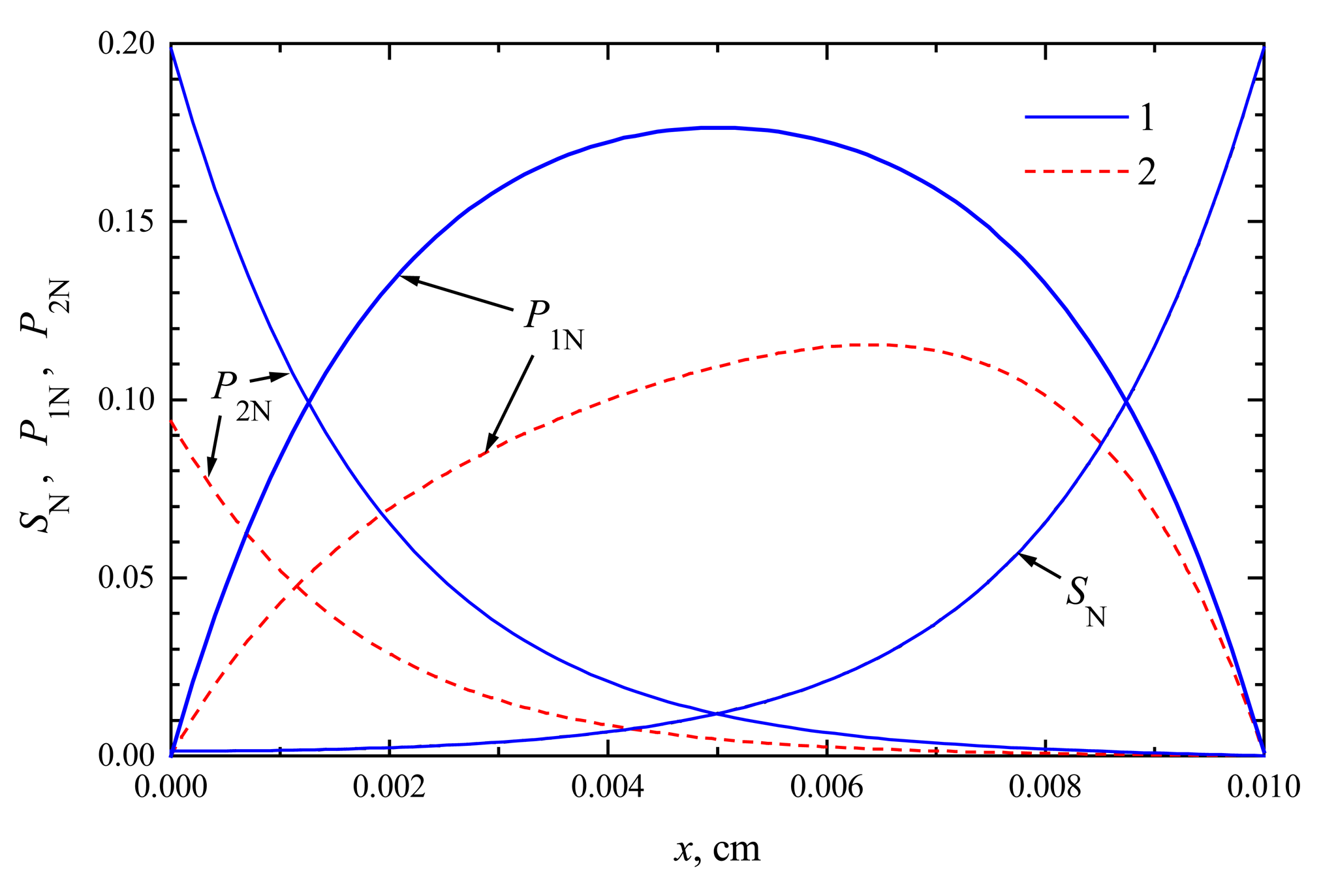
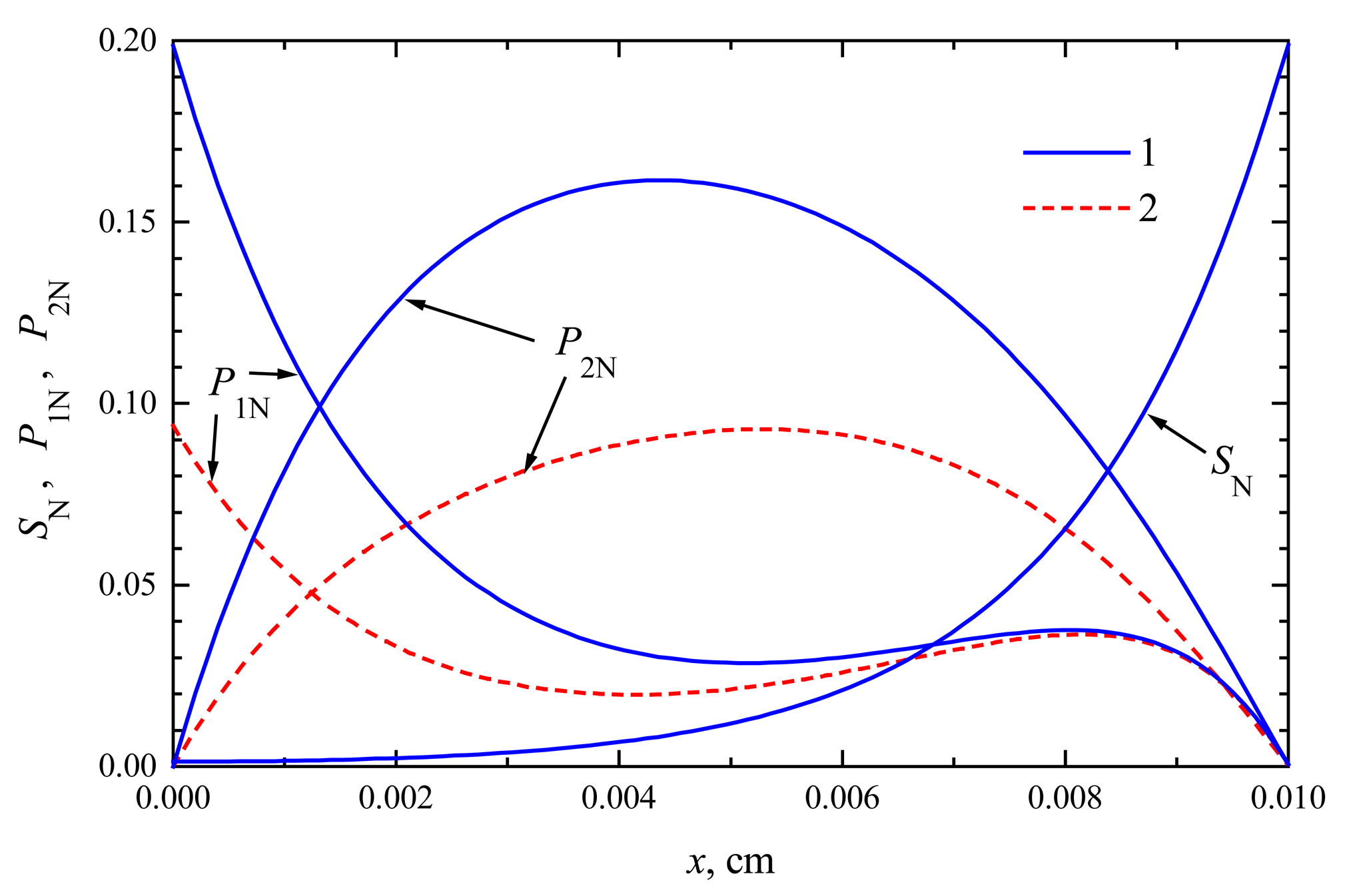
The concentration profiles in Figs. 1, 2 are shown at the time when the steady-state as well as 50% of the steady-state response has been reached. Note that for both biosensors the concentration of the substrate at steady-state conditions is approximately the same. At the time when the half of the steady-state response is reached, no significant difference has been observed, too. This is true in the entire enzyme layer, x ∈ [0, d]. The substrate concentration is described by equations (4), (7), (9) and (10), which are valid in both modes of biosensor action. This explains the similarity of substrate concentration in both modes.

The steady-state current is similar for both types of biosensors, I_CEC ≈ i_CEC(123) ≈ 6.23 μA/cm², I_CCE ≈ i_CCE(124) ≈ 6.09 μA/cm². The time of steady-state is also approximately the same in both these cases. At the steady-state conditions, i.e. ∂S/∂t = ∂P₁/∂t = ∂P₂/∂t = 0, because of the boundary conditions (9)-(12), the equality S(x, t) + P₁(x, t) + P₂(x, t) = S₀ holds for all x ∈ [0, d] when t → ∞. This can be observed in both Figs. 1 and 2.

The dependence of the steady-state current on the reactions rates

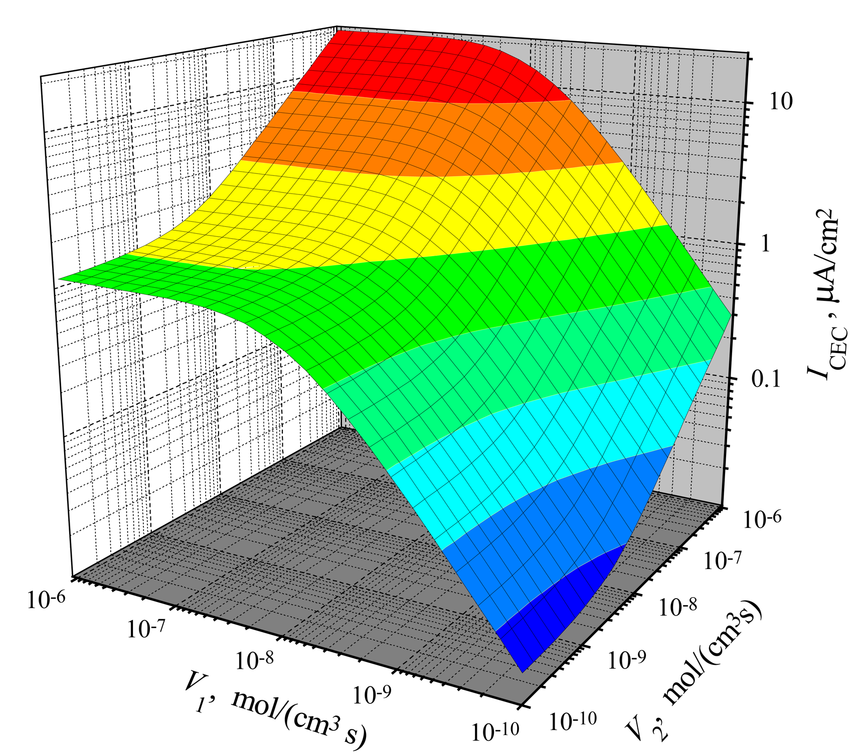
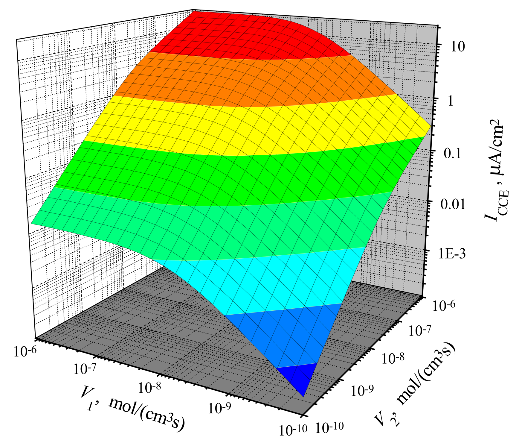
The dependence of the steady-state current on the activity of both enzymes is shown in Figs. 3, 4 for CEC and CCE modes. In calculations, V₁ and V₂ varied from 10⁻¹⁰ to 10⁻⁶ mol/(cm³s), the substrate concentration S₀ was 20 nmol/cm³, S_0N was 0.2 and membrane thickness d was 0.01 cm. One can see in Figs. 3 and 4 that I_CEC(V₁, V₂) as well as I_CCE(V₁, V₂) are monotonously increasing functions of both arguments: V₁ and V₂.

In the case of CEC mode, an application of an active enzyme E₂ (V₂ > 0) stimulates an increase of the biosensor current. In the case of V₂ = 0, the biosensor acting in CEC mode generates the current if only V₁ > 0. However, in the case of CCE mode, the appearance of an active enzyme E₂ (V₂ > 0) is a critical factor for the biosensor current. I_CCE = 0 if V₂ = 0 even if the activity of an enzyme E₁ is very high (V₁ ≫ 0). Because of this, at low values of V₂, the steady-state current I_CCE increases very quickly with increase of V₂. That effect is noted in Figs. 3 and 4 as the surface salience. The salience of the surface I_CCE(V₁, V₂) (Fig. 4) is more noticeable than the salience of the surface I_CEC(V₁, V₂) (Fig. 3).

Consequently, when V₂ → 0 at any V₁ > 0, in the CEC mode: I_CCE(V₁, V₂) → 0, while in another mode (CEC) of triggering: I_CEC(V₁, V₂) → I_CEC(V₁, 0) = I_CE(V₁). On the other hand, Figs. 3 and 4 show, that I_CEC(V₁, V₂) ≈ I_CCE(V₁, V₂) at a high maximal enzymatic rate V₂.

The dependence of the amplification on the reactions rates

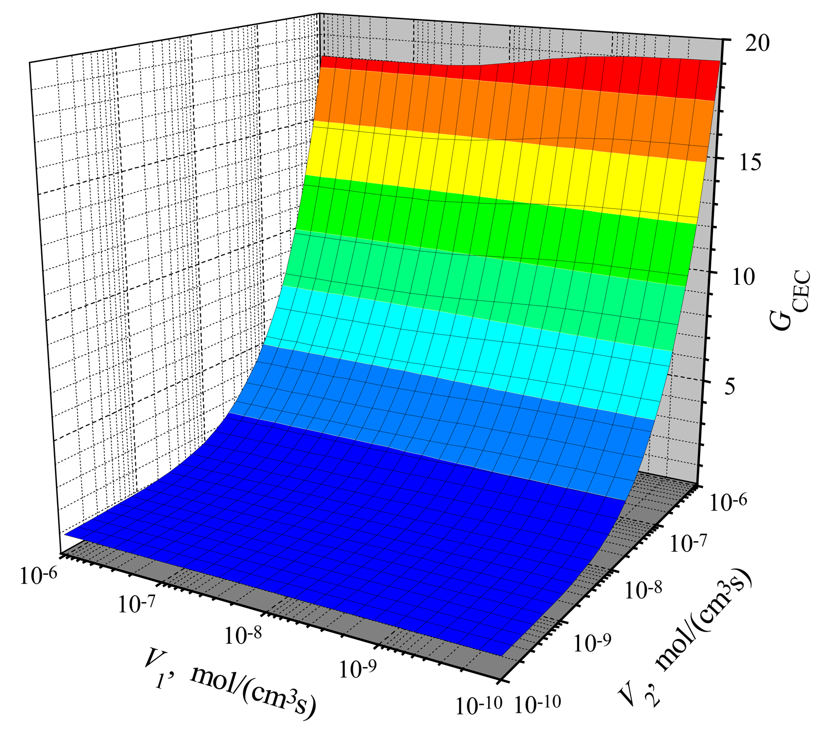
To investigate the effect of the amplification, I_CE(V₁) has been calculated at the same conditions as above. Having I_CEC(V₁, V₂), I_CCE(V₁, V₂) and I_CE(V₁), we calculated the gains G_CEC(V₁, V₂) and G_CCE(V₁, V₂). Results of calculations are depicted in Figs. 5 and 6. One can see in both figures that the gain increases with increase of V₂. The increase is especially notable at high values of V₂. The variation of V₁ on the response gain is slight by only. The gain varies from 18.0 to 19.1 at V₂ = 1 μmol/(cm³s) in both action modes: CEC and CCE.

Comparing the gain in the CEC mode (Fig. 5) with the gain in the CCE mode (Fig. 6), one can notice a significant difference at low values of V₂. The gain G_CEC starts to increase from about unity, while G_CCE at low values of V₂ (V₂ < ≈ 1 nmol/(cm³s)) is even less than unity. It means that in the case of low activity of enzyme E₂, the steady-state current of a biosensor is acting in the CCE mode even less than the steady-state current of a biosensor acting in the CE mode at the same conditions.

From the model of the CCE biosensor follows that P₂(x, t) ≈ 0 when V₂ → 0. Consequently, G_CCE(V₁, V₂) → 0 when V₂ → 0 at any V₁ > 0, while in the CEC mode: G_CEC(V₁, V₂) → 1 when V₂ → 0. On the other hand, Figs. 5 and 6 show, that G_CEC(V₁, V₂) ≈ G_CCE(V₁, V₂) at a high maximal enzymatic rate V₂, e.g. at V₂ = 1 μmol/(cm³s).

The dependence of the amplification on the substrate concentration

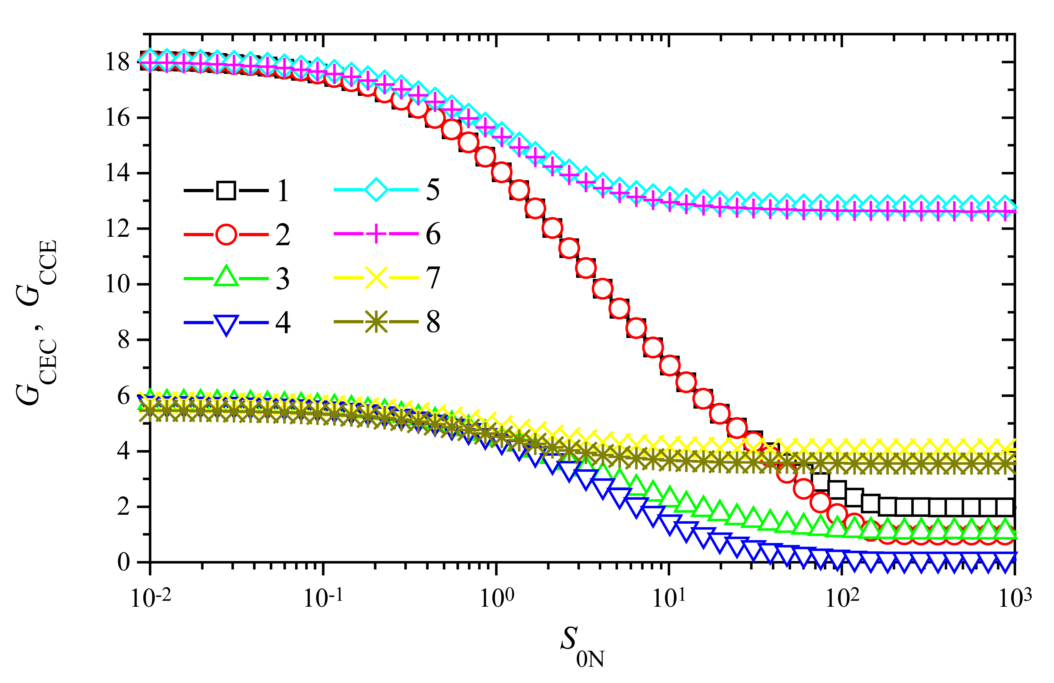
To investigate the dependence of the signal gain on the substrate concentration S₀, the response of biosensors varying S₀ from 10⁻¹⁰ to 10⁻⁴ mol/cm³ was simulated. Since the gain of trigger biosensors is significant only at a relatively high maximal enzymatic rate V₂ of enzyme E₂ (Figs. 5 and 6), we employed the following two values of V₂: 10⁻⁶ and 10⁻⁷ mol/(cm³s). We chose also two different values of the maximal enzymatic rate V₁ of enzyme E₁: 10⁻⁶ and 10⁻⁸ mol/(cm³s). Since the influence of V₁ on the signal gain is not so significant as that of V₂, the chosen two values of V₁ differ in two orders of magnitude while values of V₂ differ only in one. The results of calculations at the enzyme membrane thickness d = 0.01 cm are depicted in Fig. 7.

As one can see in Fig. 7, the behaviour of the signal gain versus the substrate concentration is very similar for both modes of the biosensor action: CEC and CCE. Some noticeable difference between values of G_CEC and G_CCE is observed at high substrate concentrations only, S_0N > 1. However, in a case of a higher value of V₂, V₂ = 10⁻⁶ mol/(cm³s), and a lower V₁, V₁ = 10⁻⁸ mol/(cm³s), no noticeable difference is observed between values of G_CEC (curve 5 in Fig. 7) and G_CCE (curve 6 in Fig. 7) in the entire domain of substrate concentration. A very similar effect can be noticed at the same value of V₁, V₁ = 10⁻⁶ mol/(cm³s), and a ten times higher value of V₂, V₂ = 10⁻⁷ mol/(cm³s), curves 7 and 8.

Fig. 7 shows the significant importance of the maximal enzymatic rate V₂ to both signal gains: G_CEC and G_CCE. Such an importance is especially perceptible at low and moderate concentrations of substrate, S_0N < 1. At S_0N < 0.1 and V₂ = 1 μmol/(cm³s) due to the amplification, the steady-state current increases up to about 18 times (G_CEC ≈ G_CCE ≈ 18). However, at the same S_0N and ten times lower value of V₂, the gain is about three times less, G_CEC ≈ G_CCE ≈ 5.7. Consequently, at low substrate concentrations, S_0N < 0.1, and wide range of the maximal enzymatic rate V₁, the tenfold reduce of V₂ reduces the signal gain about three times. This property is valid for both modes of triggering: CEC and CCE.

When increasing the substrate concentration, the signal gain starts to decrease when S_0N becomes greater than unity (Fig. 7), i.e. when S₀ > K₁ = K₂. However, the decrease is perceptible in cases of a high enzymatic rate V₁ only. At low activity of enzyme E₁ when V₁ = 1 nmol/(cm³s), the gain varies less than 30% for both values of V₂: 10 and 100 nmol/(cm³s). Additional calculations showed, that at a less activity of enzyme E₁ when V₁ = 10⁻¹⁰ mol/(cm³s), the gain practically does not vary changing the substrate concentration in the domain. Because of a very stable amplification at a wide range of substrate concentration, the usage of biosensors acting in a trigger mode is especially reasonable at a relatively low maximal enzymatic activity (rate V₁) of enzyme E₁ and a high activity (rate V₂) of enzyme E₂. In the cases of relatively high maximal enzymatic activity V₁ the signal amplification is stable only for low concentrations of the substrate.

Additional calculations showed that the signal gain vanishes fast with the decrease of the enzymatic activity V₂ of enzyme E₂. For example, in the case of V₂ = 1 nmol/(cm³s) the gain becomes less than 2 even at a low substrate concentration, G_CEC ≈ 1.91, G_CCE ≈ 1.3 at S_0N = 0.01. This effect is also observed in Figs. 5 and 6. Calculations approved the property that the tenfold reduce of V₂ reduces the signal gain about three times is valid at a wide range, also of V₂.

A similar dependence of the signal gain on the substrate concentration was observed in the case of an amperometric enzyme electrode with immobilized laccase, in which a chemical amplification by cyclic substrate conversion takes place in a single enzyme membrane [15]. In the case of the biosensor with substrate cyclic conversion, the signal gain of 36 times was observed at the maximal enzymatic rate of 1 μmol/(cm³s) and the membrane thickness of 0.02 cm. For comparison of that gain with the gain achieved in the trigger mode, we calculate G_CEC and G_CCE for the enzyme membrane of thickness d = 0.02 cm. The result of the calculation showed the amplification, G_CEC ≈ G_CCE ≈ 34 at V₁ = V₂ = 1 μmol/cm³s, d = 0.02 cm, very similar to the amplification noticed in [15,16].

The effect of the enzyme membrane thickness on the amplification

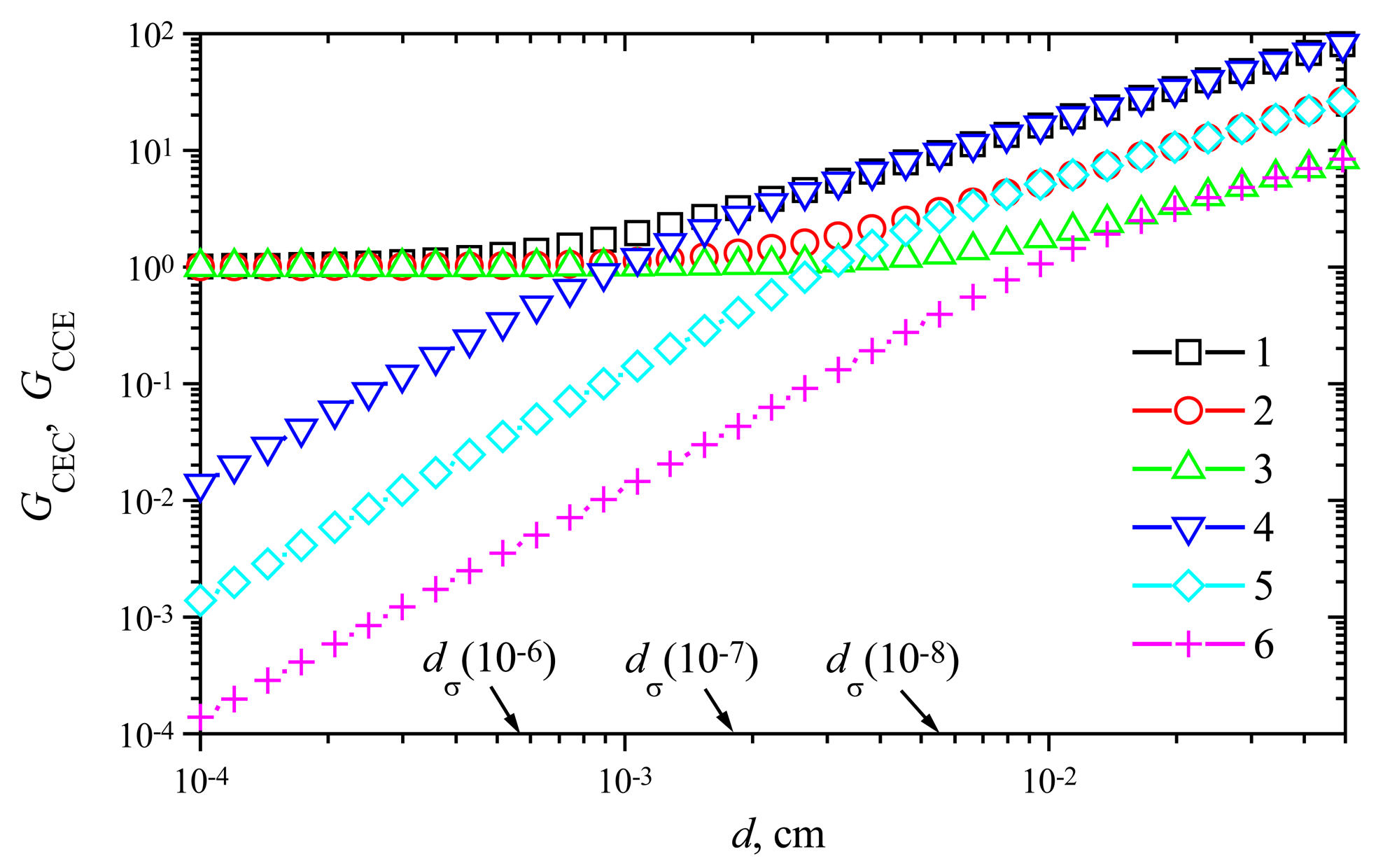
The steady-state current of membrane biosensors significantly depends on the thickness of the enzyme layer [6,16,24,27]. The steady-state time varies even in orders of magnitude. To investigate the dependence of the signal gain on the membrane thickness d, the response of biosensors varying d from 0.0001 to 0.05 cm at different maximal enzymatic rate V₁ of enzyme E₁ and rate V₂ of enzyme E₂ was simulated.

Fig. 8 shows the signal gains G_CEC and G_CCE versus the membrane thickness d at the maximal enzymatic rate V₁ = 1 μmol/(cm³s) and three values of the rate V₂: 1, 10 and 100 nmol/(cm³s). Comparing the gain G_CEC with G_CCE, one can notice valuable differences in behaviour of the signal gains. In the case of a CEC biosensor action, no notable amplification is observed in cases of a thin enzyme membrane (d < 10⁻³ cm). A more distant increase of the thickness causes an increase of the gain G_CEC. The thickness at which G_CEC starts to increase, depends on the maximal enzymatic rate V₂.

The response of amperometric biosensors is known to be under mass-transport control if the diffusion modulus σ² is greater than unity, otherwise the enzyme kinetics controls the response:

$${\sigma }^2=\frac{V_{max}{d}^2}{D_{\text{S}}{K}_{\text{M}}}$$

(32)

where V_max is the maximal enzymatic rate and K_M is the Michaelis constant. Since the diffusion coefficient D_S and K_M = K₁ = K₂ are constant in all our numerical experiments as defined in (30) and the behaviour of biosensors acting in a trigger mode is mainly determined by the enzymatic rate V_2, (Figs. 5 and 6) the thickness d_σ of the enzyme layer as a function of V₂ at which σ² = 1 has been introduced:

$$d_{\sigma }(V_2)=\sqrt{\frac{D_{\text{S}}{K}_2}{V_2}}=\sqrt{\frac{3\times {10}^{-13}}{V_2}}$$

(33)

Comparing the value d_σ(10⁻⁶) ≈ 5.5×10⁻⁴ cm with the membrane thickness at which the gain G_CEC starts to increase V₂ = 10⁻⁶ mol/(cm³s), one can notice that the amplification becomes noticeable when the mass transport by diffusion starts to control the biosensor response. As one can see in Fig. 8, this effect is also valid for two other values of the maximal enzymatic rate V₂: 10 and 100 nmol/(cm³s). However, this is valid in the case of the biosensor acting in the CEC mode only. In the case of CCE mode, the gain G_CCE increases notably with increase of the thickness d in the entire domain. G_CCE is approximately a linear increasing function of d. However, the real amplification takes place in cases of relatively thick membranes only, G_CCE > 1 if only d > ≈2d_σ. As it was noticed above (see Fig. 6), the steady-state current of the biosensor acting in the CCE mode may be even significantly less than the steady-state current of the corresponding biosensor acting in the CE mode at the same conditions. In a case of a relatively thick enzyme membrane, the gain G_CCE equals approximately to G_CEC, G_CCE ≈ G_CEC.

Using a computer simulation, we calculated more precisely the thickness d_G of the enzyme membrane at which G_CCE = 1 for different enzymatic rates V₂. Accepting V₁ = 1 μmol/(cm³s) it was found that d_G ≈ 0.0009 at V₂ = 100, d_G ≈ 0.003 at V₂ = 10, and d_G ≈ 0.009 cm at V₂ = 100 nmol/(cm³s). These values of the membrane thickness compare favourably with values of the thickness d_max at which the steady-state current as a function of the membrane thickness d gains the maximum [24]:

$$d_{max}=\frac{1}{1.5055}\sqrt{\frac{D_{\text{S}}{K}_{\text{M}}}{V_{max}}}$$

(34)

Consequently, for a low substrate concentration the thickness d_G of the enzyme membrane at which G_CEC = 1 can be precisely enough expressed as d_G ≈ 1.5 d_σ, where d_σ was defined in (33). Additional calculations showed that this property is valid for wide ranges of both maximal enzymatic rates: V₁ and V₂, if only the normalized substrate concentration S_0N is less than unity.

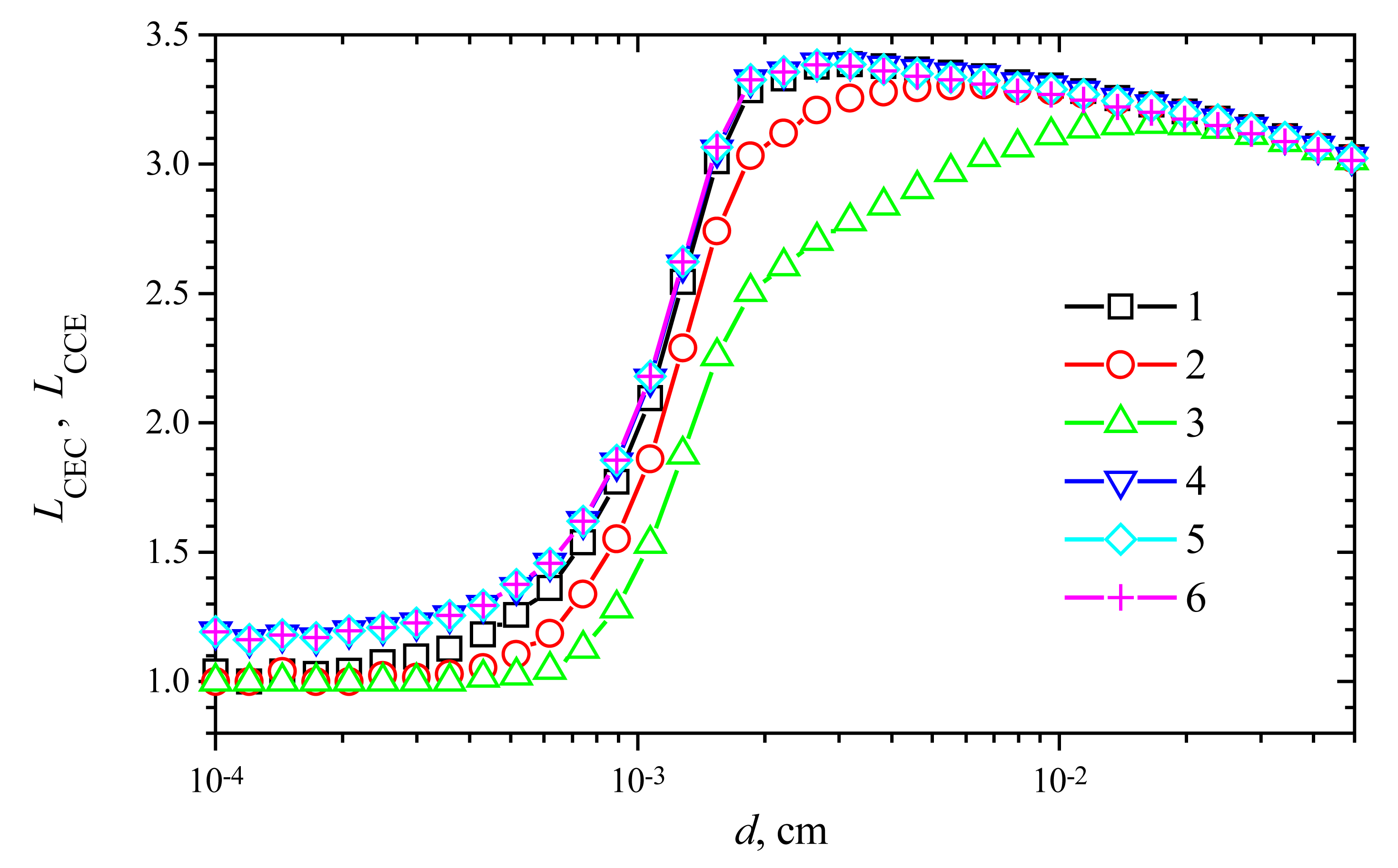
The effect of the membrane thickness on the response time

For comparing the time of a steady-state amplified biosensor response with the steady-state time of the response without amplification, we introduce a prolongation (L) of the response time as a ratio of the steady-state time of the trigger biosensor to the steady-state time of the corresponding CE biosensor:

$$\begin{array}{cc}{L}_{\text{m}}(V_1,V_2)=\frac{T_{\text{m}}(V_1,V_2)}{T_{\text{CE}}(V_1)}=\frac{T_{\text{m}}(V_1,V_2)}{T_{\text{m}}(V_1,0)},& m=\text{CEC},\text{CCE}\end{array}$$

(35)

where T_m(V₁, V₂) is the steady-state time of the triggering biosensor acting in mode m at the maximal activity V_i of the enzyme E_i, m = CEC, CCE, i = 1, 2, T_CE(V₁) is the steady-state time of the corresponding CE biosensor at the maximal enzymatic rate V₁. Since the action of the CE biosensor can be simulated as an action of a CEC biosensor accepting V₂ = 0, we assume T_CE(V₁) = T_CEC(V₁, 0).

Fig. 9 shows the change of the response time versus the membrane thickness d at V₁ = 1 μmol/(cm³s) and different values of V₂. One can see in Fig. 9, in all the presented cases, the prolongation of the response time (L_CEC as well as L_CCE) is a non-monotonous function of the thickness d. A shoulder on curves is especially noticeable at high maximal enzymatic rates. A similar effect was noticed in the case of biosensors with substrate cyclic conversion [16] and during the oxidation of β-nicotinamide adenine dinucleotide (NADH) at poly(aniline)-coated electrodes [28].

In the cases of thin enzyme membranes (d < 0.001 cm), the prolongation of the response time is insignificant. However, increasing the membrane thickness, the response time prolongation increases up to 3.4 times in both modes: CEC and CCE.

In the case of the CEC mode, the slight influence of the maximal enzymatic rate V₂ on L_CEC can be noticed in Fig. 9, while no notable influence of V₂ on L_CCE is observed in the case of CCE action mode. Additional calculations showed that the response time prolongation slightly depends on the substrate concentration S₀ as well as the maximal activity V₁ of the enzyme E₁.

Conclusions

The mathematical model (4)-(13) of the biosensor action was used to investigate the dynamics of the response of biosensors utilizing a trigger enzymatic reaction followed by the electrochemical and enzymatic product cyclic conversion (CEC scheme (1)-(3)), while the model (19)-(21), (7)-(12), (22) was applied as a framework to investigate the behaviour of biosensors utilizing a trigger enzymatic reaction followed by the enzymatic and electrochemical conversion of the product (CCE scheme (16)-(18)).

The steady-state current I_CEC of a biosensor acting in the CEC mode and the steady state current I_CCE of a biosensor acting in the CCE mode are monotonous by increasing functions of both maximal enzymatic rates: V₁ and V₂ of enzymes E₁ and E₂, respectively (Figs. 3 and 4). The corresponding gains in sensitivity, G_CEC and G_CCE, of trigger biosensors were determined mainly by the enzymatic rate V₂ (Figs. 5 and 6). The enzymatic activity V₂ is a critical factor for the biosensor current in the case of CCE mode, I_CCE → 0 as well as G_CCE → 0 if V₂ → 0. In the case of a CEC biosensor, the decrease of activity V₂ causes the decrease in gain G_CEC; however, G_CEC stays greater than unity, G_CEC → 1 if V₂→ 0.

Both signal gains, G_CEC and G_CCE, are most significant when the normalized concentration S_0N of the substrate is less than unity (Fig. 7). However, a stable and noticeable amplification (up to dozens of times) at a wide range of substrate concentration is achieved in the case of a relatively low maximal enzymatic activity (rate V₁) of enzyme E₁ and high activity (rate V₂) of enzyme E₂. In the cases of relatively high maximal enzymatic activity V₁, the signal amplification is stable only for low concentrations of the substrate.

In both biosensors acting modes, an insignificant amplification of the signal is observed if the diffusion modulus σ², calculated with the enzymatic rate V₂, is less than unity, i.e. the kinetics of enzyme E₂ controls the biosensor response. The gain G_CCE becomes even significantly less than unity if σ² ≪ 1. For this type of biosensors, at a low substrate concentration, S_0N < 1, the gain G_CCE exceeds unity only when σ > ≈ 1.5.

In the cases where the significant amplification of the signal of a triggering biosensor is achieved, the response time is up to several times longer than the response time of the corresponding biosensor acting without triggering (Fig. 9).

The models developed are permitted to build new trigger biosensors (in particular, by utilizing the CCE scheme). A highly sensitive hydrogen peroxide biosensor is under development and signal amplification has found the experimental confirmation.

References

- Blaedel, W.J.; Boguslaski, R.C. A chemical amplification in analysis: a review. Anal. Chem. 1978, 50, 1026. [Google Scholar]
- Kulys, J. The development of new analytical systems based on biocatalysts. Anal. Lett. 1981, 14(B6), 377. [Google Scholar]
- Schubert, F.; Kirstein, D.; Schröder, K.L.; Scheller, F.W. Enzyme electrodes with substrate and co-enzyme amplification. Anal. Chim. Acta 1985, 169, 391. [Google Scholar]
- Scheller, F.; Renneberg, R.; Schubert, F. Coupled enzyme reactions in enzyme electrodes using sequence, amplification, competition and anti-interference principles. In Methods in Enzymology; Academic Press: New York, 1988; Volume 137, p. 29. [Google Scholar]
- Kulys, J.J.; Vidziunaite, R.A. Amperometric enzyme electrodes with chemically amplified response. In Bioinstrumentation; Wise, D.L., Ed.; Butterwoths, 1990; p. 1263. [Google Scholar]
- Wollenberger, U.; Lisdat, F.; Scheller, F.W. Frontiers in Biosensorics 2, Practical Applications; Birkhauser Verlag: Basel, 1997. [Google Scholar]
- Streffer, K.; Kaatz, H.; Bauer, C.G.; Makower, A.; Schulmeister, T.; Scheller, F.W.; Peter, M.G.; Wollenberger, U. Application of a sensitive catechol detector for determination of tyrosinase inhibitors. Anal. Chim. Acta 1998, 362, 81. [Google Scholar]
- Fuhrmann, B.; Spohn, U. An enzymatic amplification flow injection analysis (FIA) system for the sensitive determination of phenol. Biosens. Bioelectron. 1998, 13, 895. [Google Scholar]
- Kulys, J.J.; Sorochinski, V.V.; Vidziunaite, R.A. Transient response of bienzyme electrodes. Biosensors 1986, 2, 135. [Google Scholar]
- Schulmeister, T. Mathematical treatment of concentration profiles and anodic current of amperometric enzyme electrodes with chemically-amplified response. Anal. Chim. Acta 1987, 201, 305. [Google Scholar]
- Sorochinskii, V.V.; Kurganov, B.I. Steady–state kinetics of cyclic conversions of substrate in amperometric bienzyme sensors. Biosens. Bioelectron. 1996, 11, 225. [Google Scholar]
- Schulmeister, T.; Rose, J.; Scheller, F.W. Mathematical modelling of exponential amplification in membrane-based enzyme sensors. Biosens. Bioelectron. 1997, 12, 1021. [Google Scholar]
- Malinauskas, A.; Kulys, J. Alcohol, lactate and glutamate sensors based on oxidoreductases with regeneration of nicotinamide adenine dinucleotide. Anal. Chim. Acta 1978, 98, 31. [Google Scholar]
- Kulys, J.; Schmid, R.D. A sensitive enzyme electrode for phenol monitoring. Analytical Letters 1990, 23(4), 589. [Google Scholar]
- Kulys, J.; Vidziunaite, R. Amperometric biosensors based on recombinant laccases for phenols determination. Biosens. Bioelectron. 2003, 18, 319. [Google Scholar]
- Baronas, R.; Kulys, J.; Ivanauskas, F. Modelling amperometric enzyme electrode with substrate cyclic conversion. Biosens. Bioelectron. 2004, 19, 915. [Google Scholar]
- Della Ciana, L.; Bernacca, G.; Bordin, F.; Fenu, S.; Garetto, F. Highly sensitive amperometric measurement of alkaline phosphatase activity with glucose oxidase amplification. J. Electronal. Chem. 1995, 382, 129. [Google Scholar]
- Nistor, C.; Rose, A.; Wollenberger, U.; Pfeiffer, D.; Emnéus, J. A glucose dehydrogenase biosensor as an additional signal amplification step in an enzyme-flow immunoassay. Analyst 2002, 127, 1076. [Google Scholar]
- Razumas, V.J.; Kulys, J.J.; Malinauskas, A.A. Kinetic amperometric determination of hydrolase activity. Anal. Chim. Acta 1980, 117, 387. [Google Scholar]
- Crank, J. The Mathematics of Diffusion, 2nd ed.; Clarendon Press: Oxford, 1975. [Google Scholar]
- Britz, D. Digital simulation in electrochemistry, 2nd ed.; Springer–Verlag: Berlin, 1988. [Google Scholar]
- Bartlett, P.N.; Pratt, K.F.E. Modelling of processes in enzyme electrodes. Biosens. Bioelectron. 1993, 8, 451. [Google Scholar]
- Yokoyama, K.; Kayanuma, Y. Cyclic voltammetric simulation for electrochemically mediated enzyme reaction and determination of enzyme kinetic constants. Anal. Chem. 1998, 70, 3368. [Google Scholar]
- Baronas, R.; Ivanauskas, F.; Kulys, J. The influence of the enzyme membrane thickness on the response of amperometric biosensors. Sensors 2003, 3, 248. [Google Scholar]
- Ames, W.F. Numerical Methods for Partial Differential Equations, 2nd ed.; Academic Press: New York, 1977. [Google Scholar]
- Press, W.H.; Flannery, B.P.; Teukolsky, S.A.; Vetterling, W.T. Numerical Recipes in C: The Art of Scientific Computing; Cambridge University Press: Cambridge, 1993. [Google Scholar]
- Turner, A.P.F.; Karube, I.; Wilson, G.S. Biosensors: Fundamentals and Applications; Oxford University Press: Oxford, 1987. [Google Scholar]
- Bartlett, P.N.; Birkin, P.R.; Wallace, E.N.K. Oxidation of β-nicotinamide adenine dinucleotide (NADH) at poly(aniline)-coated electrodes. J. Chem. Soc., Faraday Trans. 1997, 93, 1951. [Google Scholar]
Figure 1.
The profiles of the normalized concentrations of substrate (SN) and products (P1N, P2N) in the enzyme membrane of a CEC biosensor at the maximal enzymatic rate V1 = V2 = 100 nmol/(cm3s), S0N = 0.2, d = 0.01 cm. The profiles show the concentrations at the steady-state time t = 123 s (1) and half time t = 12 s (2).
Figure 2.
The profiles of the normalized concentrations in the enzyme membrane of a CCE biosensor at time t = 124 s (1) when the steady-state is reached and t = 12 s (2) at the half of it. Other parameters and notation are the same as in Fig. 1.
Figure 3.
The steady-state current versus the maximal enzymatic rates V1 and V2 of the biosensor acting in CEC mode, S0N = 0.2, d = 0.01 cm.
Figure 4.
The steady-state current versus V1 and V2 of the biosensor acting in CCE mode at the same conditions as in Fig. 3.
Figure 5.
The signal gain GCEC versus the maximal enzymatic rates V1 and V2 of the biosensor acting in the CEC mode at the conditions defined in Fig. 3.
Figure 6.
The signal gain GCCE versus the maximal enzymatic rates V1 and V2 of the biosensor acting in the CCE mode at the conditions defined in Fig. 3.
Figure 7.
The signal gains GCEC (1, 3, 5, 7) and GCCE (2, 4, 6, 8) vs. the substrate concentration S0N at the maximal enzymatic rates V1: 100 (1-4), 1 (5-8) and V2: 100 (1, 2, 5, 6), 10 (3, 4, 7, 8) nmol/(cm3s), d = 0.01 cm.
Figure 8.
The signal gains GCEC (1-3) and GCCE (4-6) versus the membrane thickness d at three maximal enzymatic rates V2: 100 (1, 4), 10 (2, 5) and 1 (3, 6) nmol/(cm3s); V1 = 1 μmol/(cm3s), S0N = 0.2.
Figure 9.
The increase of response time LCEC (1-3) and LCCE (4-6) versus the membrane thickness d. Parameters and notation are the same as in Fig. 8.
© 2004 by MDPI ( http://www.mdpi.org). Reproduction is permitted for non-commercial purposes.
Share and Cite
MDPI and ACS Style
Baronas, R.; Kulys, J.; Ivanauskas, F. Mathematical Model of the Biosensors Acting in a Trigger Mode. Sensors 2004, 4, 20-36. https://doi.org/10.3390/s40400020
AMA Style
Baronas R, Kulys J, Ivanauskas F. Mathematical Model of the Biosensors Acting in a Trigger Mode. Sensors. 2004; 4(4):20-36. https://doi.org/10.3390/s40400020
Chicago/Turabian StyleBaronas, Romas, Juozas Kulys, and Feliksas Ivanauskas. 2004. "Mathematical Model of the Biosensors Acting in a Trigger Mode" Sensors 4, no. 4: 20-36. https://doi.org/10.3390/s40400020