Environmental Studies with the Sensor Web: Principles and Practice

Abstract

In 1997, the Sensor Web was conceived at the NASA/Jet Propulsion Laboratory (JPL) to take advantage of the increasingly inexpensive, yet sophisticated, mass consumer-market chips for the computer and telecommunication industries and use them to create platforms that share information among themselves and act in concert as a single instrument. This instrument would be embedded into an environment to monitor and even control it. The Sensor Web's purpose is to extract knowledge from the data it collects and use this information to intelligently react and adapt to its surroundings. It links a remote end-user's cognizance with the observed environment. Here, we examine not only current progress in the Sensor Web technology, but also its recent application to problems in hydrology to illustrate the general concepts involved.

Overview of the Sensor Web

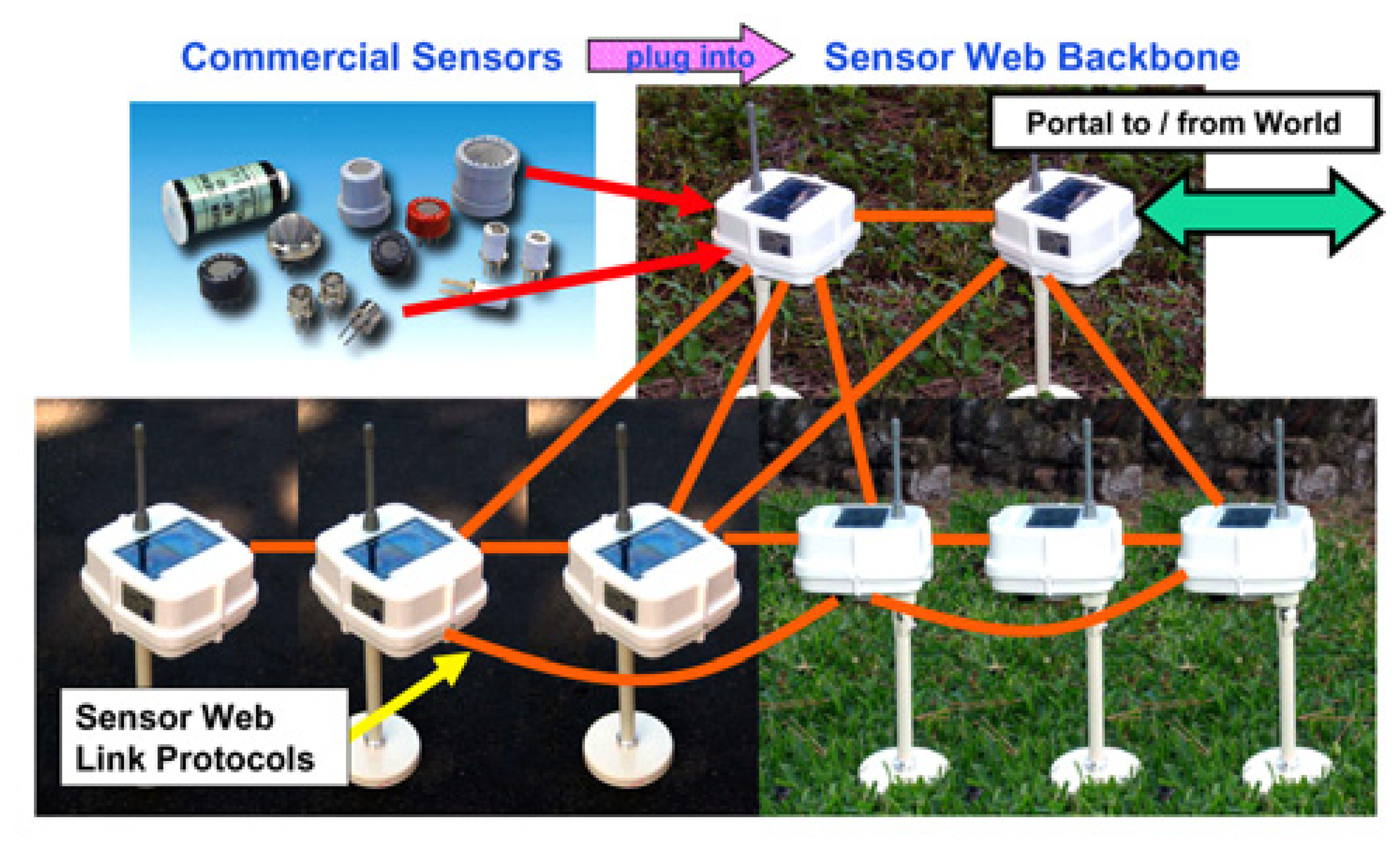
In its most general form, the Sensor Web is a macro-instrument comprised of spatially-distributed sensor platforms [1]. As shown in Figure 1, these platforms, or pods, can be orbital or terrestrial, fixed or mobile. Coordinated communication and interaction among the pods provides a local fusion of the dispersed data and results in a spatio-temporal understanding of the environment. Specific portal pods provide end-user access points for command and information flow into and out of the Sensor Web. The NASA/JPL Sensor Webs Project is currently focused on in-situ Sensor Webs, with the resulting instrument accessible, in real-time, via the Internet.

The Sensor Web's capabilities are useful in a diverse set of outdoor applications ranging from precision agriculture to perimeter security to effluent tracking. Wireless networks of sensors are often marketed as replacements for running wire to sensing points. Naturally this holds true for the Sensor Web as well, with the individual pods communicating among themselves wirelessly. However, it is more significant that the Sensor Web, with its unique global information sharing protocol, forms a sophisticated sensing tapestry that can be draped over an environment. This Sensor Web approach allows for various complex behaviors and operations such as on-the-fly identification of anomalous or unexpected events, mapping vector fields from measured scalar values and interpreting them locally, and single-pod detection of critical events which then triggers changes in the global behavior of the Sensor Web.

Wireless networks are not a new approach to environmental monitoring and it is common to find systems where remote sensors in the field communicate to central points for data processing in a star-network formation. The Sensor Web, however, is a temporally synchronous, spatially amorphous network, creating an embedded, distributed monitoring presence which provides a dynamic infrastructure for sensors. By eschewing a central point on the network, information flows everywhere throughout the instrument (see Figure 2).

So far, this sounds like a typical ad hoc, self-configuring, mesh network. Often, the ideas of hopping information around such a network are framed in terms of the power advantage gained by doing so. While this advantage certainly exists, the Sensor Web concept goes one step further: the individual pods comprising a Sensor Web are not just elements that can communicate with one another; they are elements that must communicate with one another. Whereas wireless networks are typically discussed as confederations of individual elements (like computers connected to the Internet), the Sensor Web is a single, autonomous, distributed instrument. The pods of a Sensor Web are akin to the cells of a multi-cellular organism; the primary purpose for information flow over a Sensor Web is not about getting data to an end-user, but rather to the rest of the Sensor Web itself.

By design, the Sensor Web spreads collected data and processed information throughout its entire network. As a result, there is no design criterion for routing as in more typical wireless systems. Routing, by definition, is a focused moving of information from one point to another. In contrast, information collected by a Sensor Web is spread everywhere, rendering meaningless the concept of routing on it. Instead, the communication protocol on a Sensor Web is relatively simple and is structured for both omni- and bi-directional information flows. Omni-directional communication implies no directed information flow, while bi-directional communication lets individual pods (and end-users) command other pods as well as receive information from them. Consequently, information on the Sensor Web can result from four types of data: (a) raw data sensed at a specific pod, (b) post-processed sensed data from a pod or group of pods, (c) commands entered into the distributed instrument by an external end-user, and (d) commands entered into the distributed instrument by a pod itself. The Sensor Web processes this internal information, draws knowledge from it, and reacts to that knowledge.

Since there is no specific routing of information, all pods share everything with each other. After each measurement is taken, both raw and processed information from each pod are moved throughout the Sensor Web to all other pods before the next measurement is taken. Because the Sensor Web is a single, distributed instrument, its internal operations are synchronous from pod to pod (again in contrast to more common wireless networks). In this way, the total snapshot associated with that instant in time is available to all pods on the Sensor Web. This global data sharing allows each pod to sense phenomena beyond its specific location. Pods may therefore, combine data across the Sensor Web to identify a moving front and determine its speed and direction, a task that a single-point measurement can not accomplish. Pods may also use neighbours to examine the stochastic nature of their local measurements to determine whether or not the data collected are well-behaved. Such macroscopically coordinated data processing would not be as straightforward if each pod were semi-autonomous on the network, as in typical wireless sensor systems. There is a degree of stiffness to the information flow over the Sensor Web compared to the individually directed node-to-node information threads on more typical wireless systems. The Sensor Web pods may be thought of as individual, synchronized pixels in a much larger instrument that can take snapshots at regular intervals of the entire environment in which it is embedded and each pixel is simultaneously aware of the overall picture as well as its local readings.

Sensor Web pods

A Sensor Web pod consists of five basic modules:

(1)

The radio, which links each pod to its local neighborhood. The NASA/JPL Sensor Web pods use radios operating in the 900 MHz license-free Industrial, Science and Medical (ISM) band with an upper range of ∼200 m or more. (Implicitly, we assume none of the in-situ Sensor Webs discussed here are deployed underwater, where acoustic modems severely limit bandwidth and communication range relative to these ISM radios.)

(2)

The microcontroller, which contains the system's protocols, communicates with the attached sensors, and carries out data analysis as needed.

(3)

The power system. The NASA/JPL system uses a battery pack with solar panels to keep the batteries charged. The combination of solar panels and micropower electronic design have kept Sensor Web pods operating in the field for years without requiring maintenance.

(4)

The pod packaging. This key module is often overlooked, especially for Sensor Web applications in the wild. The package must be light, durable, inexpensive, and sealed against such elements as rain, snow, salty sprays, dust storms, and local fauna. In addition, it must provide for easy and rapid mounting.

(5)

The sensor suite. This module is completely determined by the specific application. Ideally, the sensor suite will, in fact, be the prime-determining factor for the size, cost, and power requirements of a Sensor Web pod, making the Sensor Web infrastructure attractive for any application. What is considered an inexpensive or small Sensor Web pod in one application may not be viewed as such in another.

We have been conditioned by decades of experience with Moore's Law (and the technology revolution associated with it) to think that smaller is always better. There are certainly practical reasons for limiting the size of a Sensor Web pod. In an outdoor environment, smaller and lighter pods are easier to deploy since more can fit into, say, a backpack. However, shrinking pods to infinitesimal sizes is undesirable for a typical outdoor Sensor Web system. Consider the impact of size with respect to three key Sensor Web pod design issues: power, antenna size, and transducers.

An important design requirement for typical outdoor Sensor Webs is pod longevity. In many cases, deployment is only practical during certain seasons and therefore, intra-season maintenance must be avoided. As a result, maximizing the available power, by cleverly using batteries and/or energy harvesting, is critical. Batteries are often rated in terms of their energy density (watt-hours per unit volume). This is because cells can be added serially to increase total available voltage. The larger the volume of the Sensor Web pod, the more volume is available for power from any particular battery technology.

There are only two ways to maintain a given amount of battery power level available while allowing the pod volume to shrink: improve the battery technology or reduce energy use within the pod. While there are numerous efforts to provide higher energy-density power sources than are typically available (e.g,. lithium ion batteries), none are yet commercially available for consumer use. In addition, many experimental batteries have limited lifetimes. Moreover, any suitable battery technology must be essentially zero-maintenance and environmentally robust (especially to changes in temperature, both seasonal and diurnal). As for improving energy efficiency, the laws of physics require a certain power output to broadcast a given distance. Therefore, although one can lower the energy per bit involved in computation, the wireless communication puts a hard limit on how much energy will be required for the system to operate for a given pod-to-pod distance.

Now, consider energy harvesting which is typically accomplished via solar power charging secondary batteries. Here, too, the smaller the platform, the smaller the solar panels used to re-energize the system, and the smaller amount of energy that can be harvested for a given panel. Clearly, beyond a certain size, the smaller one designs a Sensor Web pod for a given set of operating parameters, the more one gives up in terms of longevity with respect to available power.

Antennas are also directly related to platform size. Again, the laws of physics dictate the appropriate antenna geometry for a given operating frequency to ensure a proper impedance match into the radiated space. As a result, while the on-board processor and radio electronics may shrink, the antenna may not if a particular communication range is required. Without proper coupling, radiation efficiency is reduced and power must be increased to the radio to maintain range. We therefore find that since most outdoor Sensor Webs required pod-to-pod ranges of at least tens of meters, indiscriminate shrinking of the individual antennas clearly compromise the telecommunication subsystem.

Lastly, consider the sensors themselves. many sensors used in outdoor field applications, though compact and inexpensive, are not micro-electromechanical system (MEMS) devices and therefore cannot be integrated into the Sensor Web pod at the chip level. As a result, for a wide variety of Sensor Web applications in an outdoor environment, the sensors will be additional components added to the basic pod platform. Clearly, there is little to be gained by continually shrinking the platform if the sensors themselves remain the limiting size element. Moreover, shrinking the platform may actually complicate the design if it becomes difficult to integrate the sensors into the pod.

As shown in Figure 3, the NASA Sensor Web pods have been developed in several sizes, including that of a gumball and that of a couple of decks of playing cards. Significantly, the gumball-sized pod dates back to 1998 [1], demonstrating, even then, that it was relatively easy to make small platforms so long as only simple measured parameters (i.e., temperature, humidity, etc.) and short pod-to-pod communication distances (i.e., order of meters) were required. Such small pods are ideal for building or factory monitoring, but less practical for outdoor environments for reasons discussed above. From this discussion, it is apparent that, while smaller pods are desirable, shrinking pods beyond a certain point leads to diminishing returns.

Fielding a Sensor Web

With the objective to do real in-situ environmental work, the NASA/JPL Sensor Webs Project has been aggressive about fielding instruments. Sensor Webs have been deployed in a large variety of demanding real-world locations for many months or even years. For example, Sensor Webs have been at the Huntington Botanical Gardens in San Marino, CA, starting with the deployment of Sensor Web 2.0 in June 2000 and continuing with Sensor Web 3.0, the first permanent wireless sensor network system to provide continuous real-time streaming data to users over the Internet, in October 2001. The Gardens continue to remain a significant test site for Sensor Web technology [1]. Information about other deployments in a variety of environments as well as real-time, streaming data from several present deployments, is available on the Internet [2].

From the experience of deploying the Sensor Web in a multitude of environments with varying conditions, it is apparent that the ease with which the system is deployed is just as critical for acceptance by end-users as are its technological aspects. With the exception of applications in battlefield theaters, most outdoor Sensor Web applications require the system to be deployed in manner that does not harm the monitored environment. For example, end users have expressed concerns that if Sensor Web pods are too small, local fauna may try to ingest them and choke. End-users also want to avoid littering their environment with hundreds of pieces of microelectronic gear.

Most applications require tracking specific pod location and it is therefore highly unlikely that pods will simply be sprinkled over large areas. In addition, coupling sensors into the environment will usually prevent such a passive deployment. For example, neither subterranean nor seismic sensors can be deployed by a sprinkling technique, as both require laborious efforts for appropriate sensor mounting. Consequently, the mounting and placement of Sensor Web pods will be an active operation and likely to be done by hand in most instances.

The methods used to mount the Sensor Web pods depend not only on the application but also the particular field site. Pod placement very close to the ground can limit transmission distance. Nevertheless, while the Huntington Garden pods are within 10 inches of the ground, they have sufficient communication power to keep an adequate pod-to-pod distance. Often, for logistical reasons, the Sensor Web pods tend to be mounted higher off the ground with the attendant benefit of increasing the wireless distance. Local terrain is rarely level which also tends to increase transmission distances. We have typically used posts (for horizontal surfaces) and brackets (for vertical surfaces) to mount the pods. These types of mounts are both small enough and light enough to bring into the field yet are sturdy enough for fixing the Sensor Web pods rigidly in place for long durations.

Sensor Web deployment at a recharge basin facility

Each year, large-scale flooding affects millions of people around the world with attendant losses of property and life. A major limitation in the mapping and characterization of catastrophic floods is an inability to monitor them in real-time. For instance, it has been historically difficult to study transient hydrologic phenomena such as storm-induced flooding, surface water movements, water infiltration, and soil moisture conditions. This limitation has had a direct impact on accurate flood prediction systems. The Sensor Web can address this deficiency by providing real-time detection and monitoring of both surface water conditions and water infiltration.

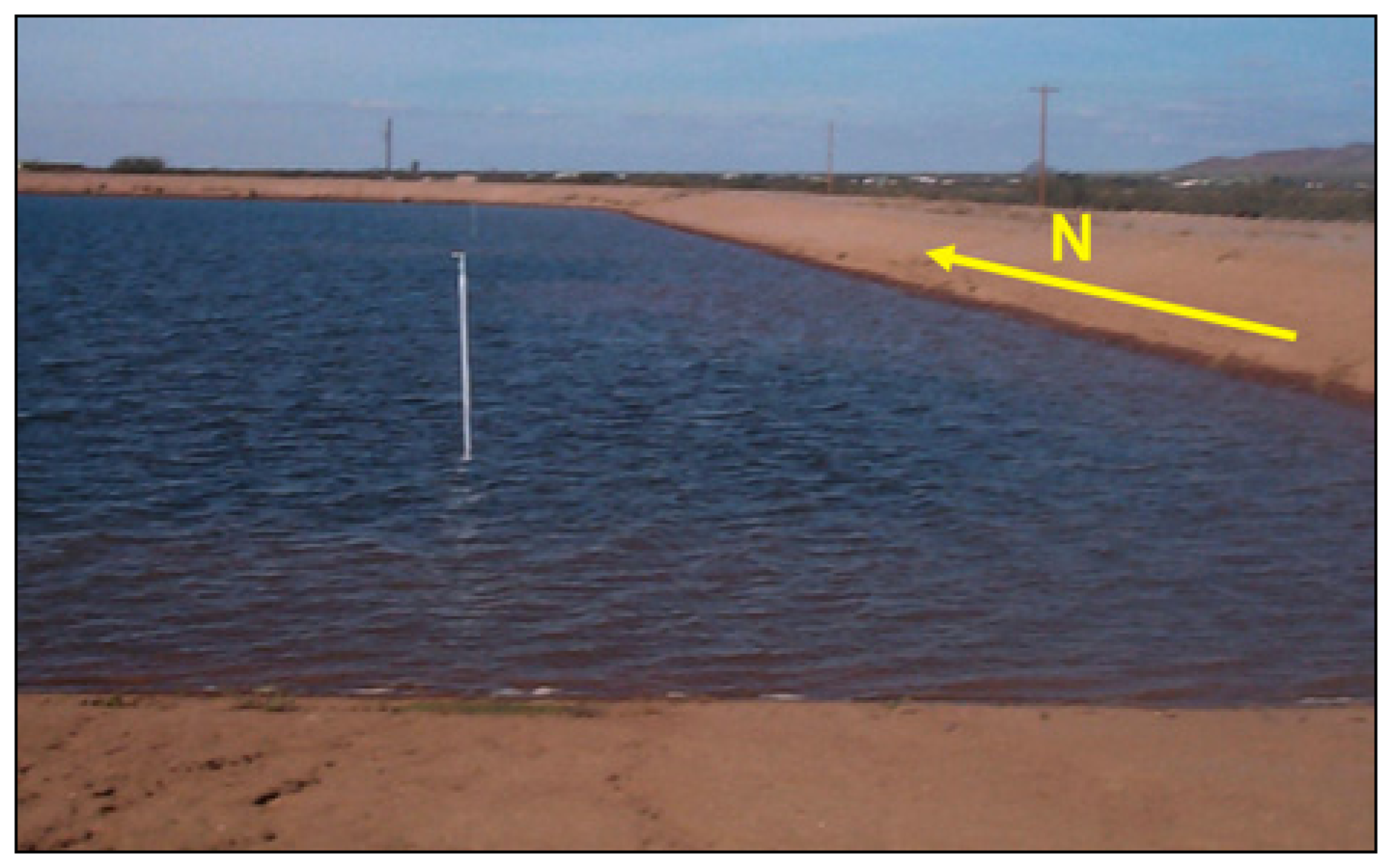
We have deployed a Sensor Web at the Central Avra Valley Storage and Recovery Project (CAVSARP) facility located west of Tucson, AZ [2,3] and shown in Figure 4. The facility is located in a desert environment of the semi-arid Southwest United States where the artificial recharge basins experience repeated flood cycles. The controlled flooding conditions at the CAVSARP facility are ideal for the investigation of various hydrologic processes. Common geomorphologic features related to flood inundation observed at the site are analogous to features often found in ancient paleolakes on both Earth and Mars and include wave-cut terraces, polygonal-patterned ground, and ridges related to drying of basin floor materials. Algal mats are also visible in some of the basins during the drying period of the flood cycle. Thus, the flood-related phenomena at the facility are of great interest to both hydrologists and terrestrial and planetary geologists.

There are several technology-related reasons for this site choice as well. The CAVSARP facility, with its controlled flood conditions, allows us to continue our efforts to develop the Sensor Web as a tool for the study of spatio-temporal phenomena. For example, the Sensor Web can track the moving flood front, follow the infiltration of water into the ground, and provide information to map and characterize the lateral and vertical extent of the floodwaters. Moreover, the extreme temperature variations of the Arizona desert (both diurnal and seasonal) provide yet another test of the Sensor Web's robustness. The deployed Sensor Web had essentially identical hardware to those of previous installations [4] and no special provisions were made for the new environment.

The recharge basins are operated cyclically to allow for routine maintenance of the surface conditions. These operations lead to periodic infilling, with a water front progressing across the basin. Once the inflow of water is shut off, the floodwaters continue to infiltrate into the ground and the drying portion of the cycle begins with the drying front reversing the original flood pattern. The basins were constructed to have a smoothly varying elevation, which declines from south to north. As a result, the north ends of the basins fill first during flooding and dry last during draining. Existing instruments in each basin provide for continuous monitoring of inflow rate at the inlet pipe and water height at the deep end. These instruments are connected to a Supervisory Control And Data Acquisition System (SCADA), allowing for remote monitoring of basin operations. A visual staff gauge is regularly read to confirm the accuracy of the water level sensors.

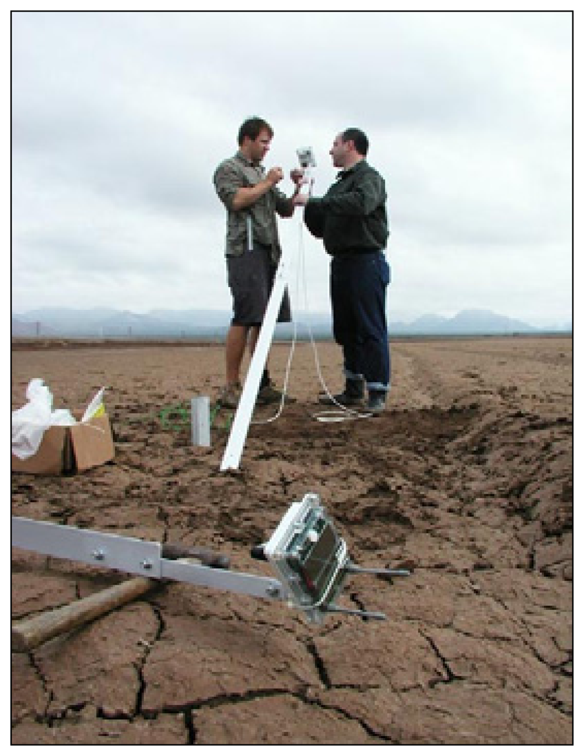
A single basin (102), measuring approximately 700×2400 ft², was strategically outfitted with 13 Sensor Web 3.2 pods, the number and placement of pods being determined by science requirements, rather than technological limitations. As shown in Figure 5, the pods were mounted on stakes to elevate them above the flood waters which can rise as high as 7 ft. (While the pods themselves are water-tight, pod-to-pod radio communication would not be possible if they were submerged.) Each pod, in addition to collecting air temperature, humidity, and light levels also collects two soil moisture readings (one at the surface and one 0.5 m below) and a surface soil temperature reading. This is accomplished by wires that run from the pod into the ground. Measurements are made at 5 minute intervals with the results being fed to the Internet in real-time (via the portal pod 0). Figure 6 shows the deployed Sensor Web during a flooding event.

Preliminary use of Sensor Web in hydrologic studies

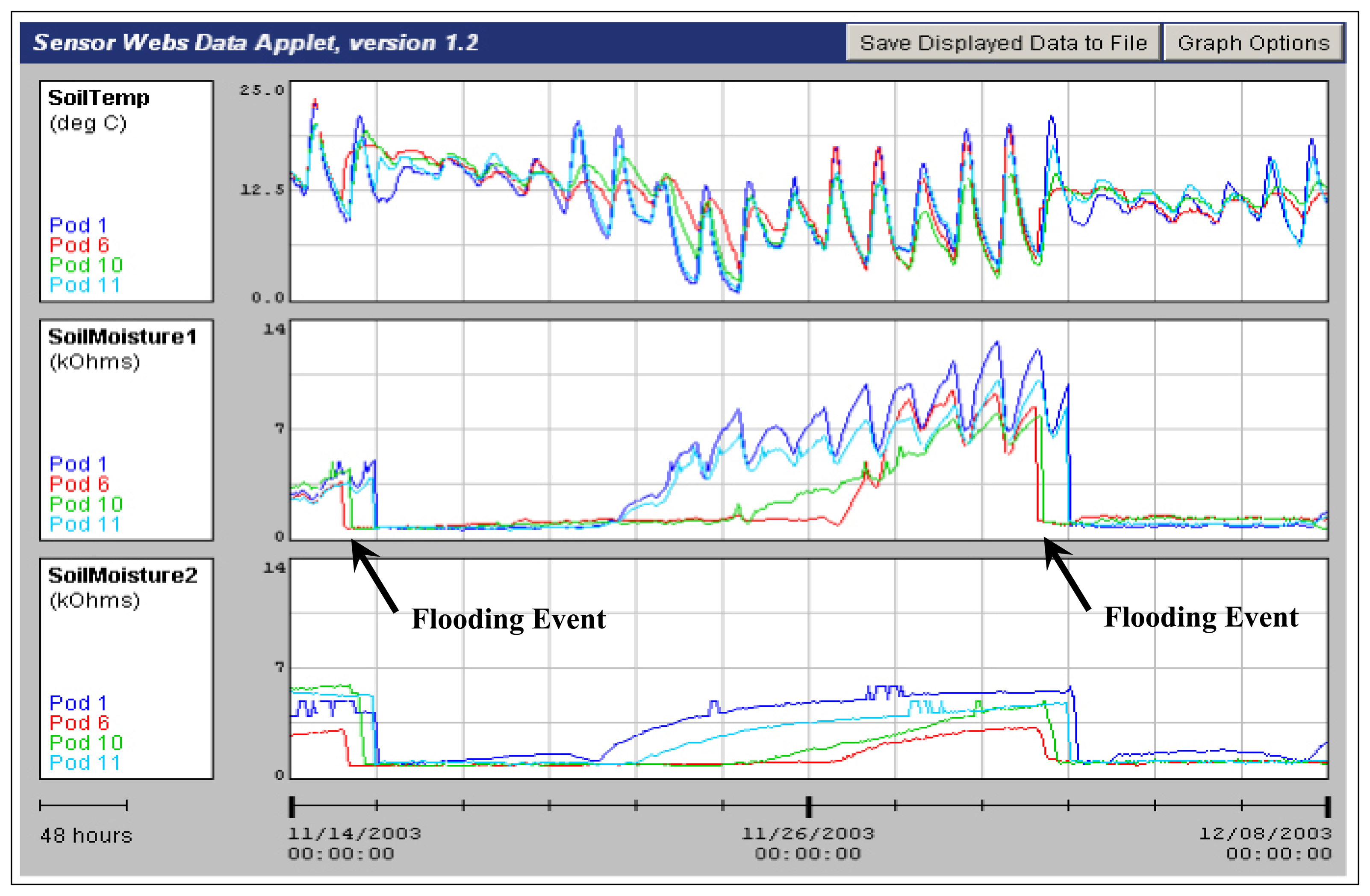
This Sensor Web has been collecting data since its deployment in November 2003. The real-time, streaming output from this system was made available via the Internet; a sample screen-capture is shown in Figure 7. Unlike remote techniques, which can only observe the basins for relatively short durations on finite schedules, the Sensor Web's data stream provides continuous information for tracking surface water motion and ground infiltration. The spatial and temporal patterns of wetting and drying can thus, be fully monitored and results incorporated into hydrological models and compared with space- and airborne-based investigations [5]. This analysis is ongoing. As a result, this Sensor Web can both augment and ground-truth the remote data traditionally used in hydrologic studies.

The repeatable nature of the flooding/drying dynamics is apparent in Figure 7. The soil moisture measurements are made with Watermark sensors [6], where electrodes embedded in a granular matrix yield a lower resistance when the surrounding soil is wetter. As a result, the raw data reveals the motion of the flooding water as sharp drops in resistance. (The diurnal cycles seen in the raw data are sensor artifacts and can be corrected with soil temperature measurements [7].) It only takes a few hours for the flood front to traverse the basin from the inlet in the northwest corner to the basin center but a much longer time (about 20 hours) to reach the basin's southwest and southeast corners. Note, too, that the water reaches the southern border relatively evenly (as indicated by pods 1 and 11), which is expected from both basin construction and the photographic evidence shown in Figure 4. Moreover, it is also clear from Figure 7 that the drying front traverses the reverse route, albeit at a much slower speed. Not surprisingly, the surface dries more thoroughly than the deeper portions of the ground.

The raw data can be downloaded using the Sensor Web's graphical user interface so that these initial observations can be further refined into more meaningful hydrologic terms. Soil moisture can be described in terms of the forces that retain the water in the soil. At equilibrium, the energy status of the water in the sensor's granular matrix is equal to the energy status of the water in the surrounding soil. The electrical resistance measured is then related to the soil water potential by the sensor-specific calibration:

$$\mathit{\text{SoilWaterPotential}}(\mathit{\text{kPa}})=-\frac{4.0963+3.213\times R}{1-0.009733\times R-0.01205\times T}$$

(1)

where R is the sensor resistance in kΩ and T is the soil temperature in °C [7].

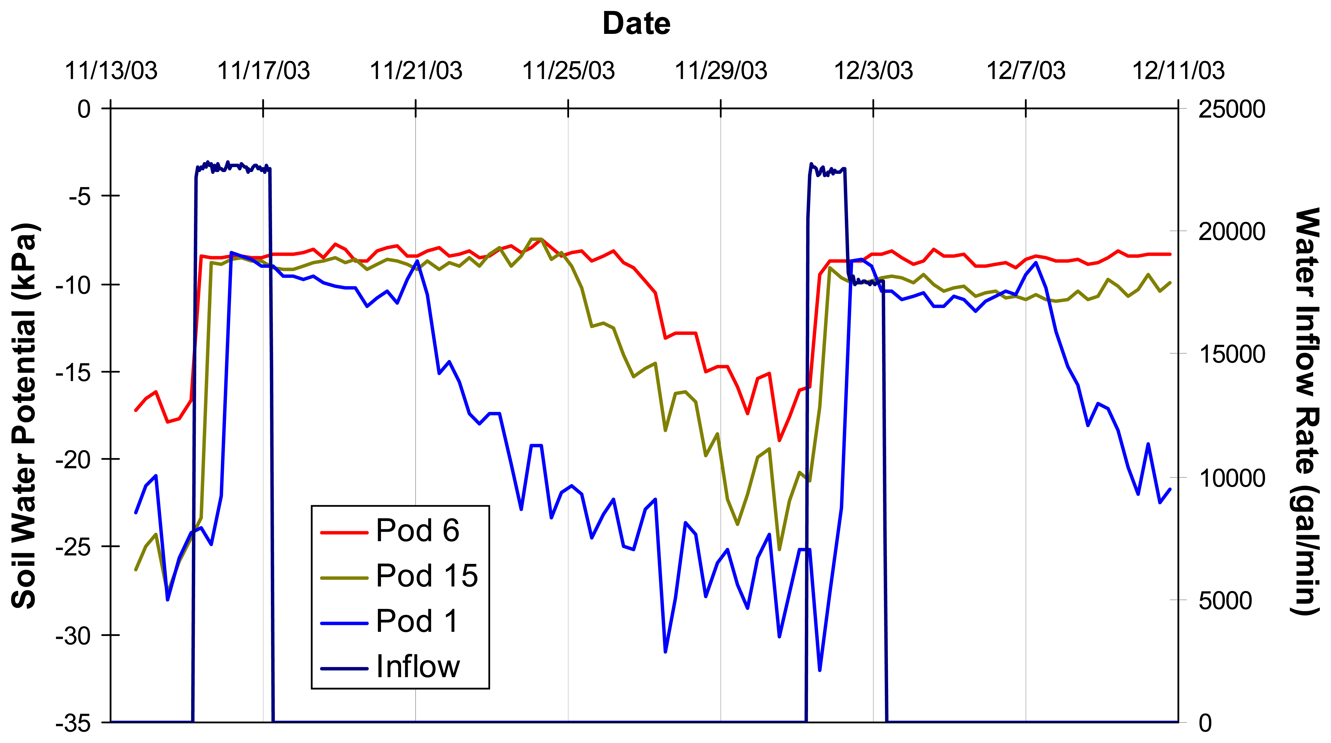
Figure 8 shows the same two flooding events of Figure 7 at a depth of 0.5 m, but with the raw data interpreted in this manner. The inlet flow is also plotted. The maximum inflow rate was approximately 22800 gal/min with the water rising, in this case, to 5.7 ft. The pods examined are on the basin's western border and, again, it is clear that a finite time is required for the moving water front to travel south from the inlet (pod 6) to the near corner (pod 1). In contrast, note how rapidly the soil moisture at depth increases at pod 6. The slight difference in the temporal aspects of soil wetting between the two flood events (most notably at pod 6) is attributable to the fact that the soil moisture sensors were planted just prior to the first flood event and therefore, the surrounding soil was disturbed and not as compacted as before sensor insertion. The second flooding event therefore, provides data for more accurate modeling. Again, the Sensor Web provides a continuous embedded monitoring presence which leads to a more refined picture of events.

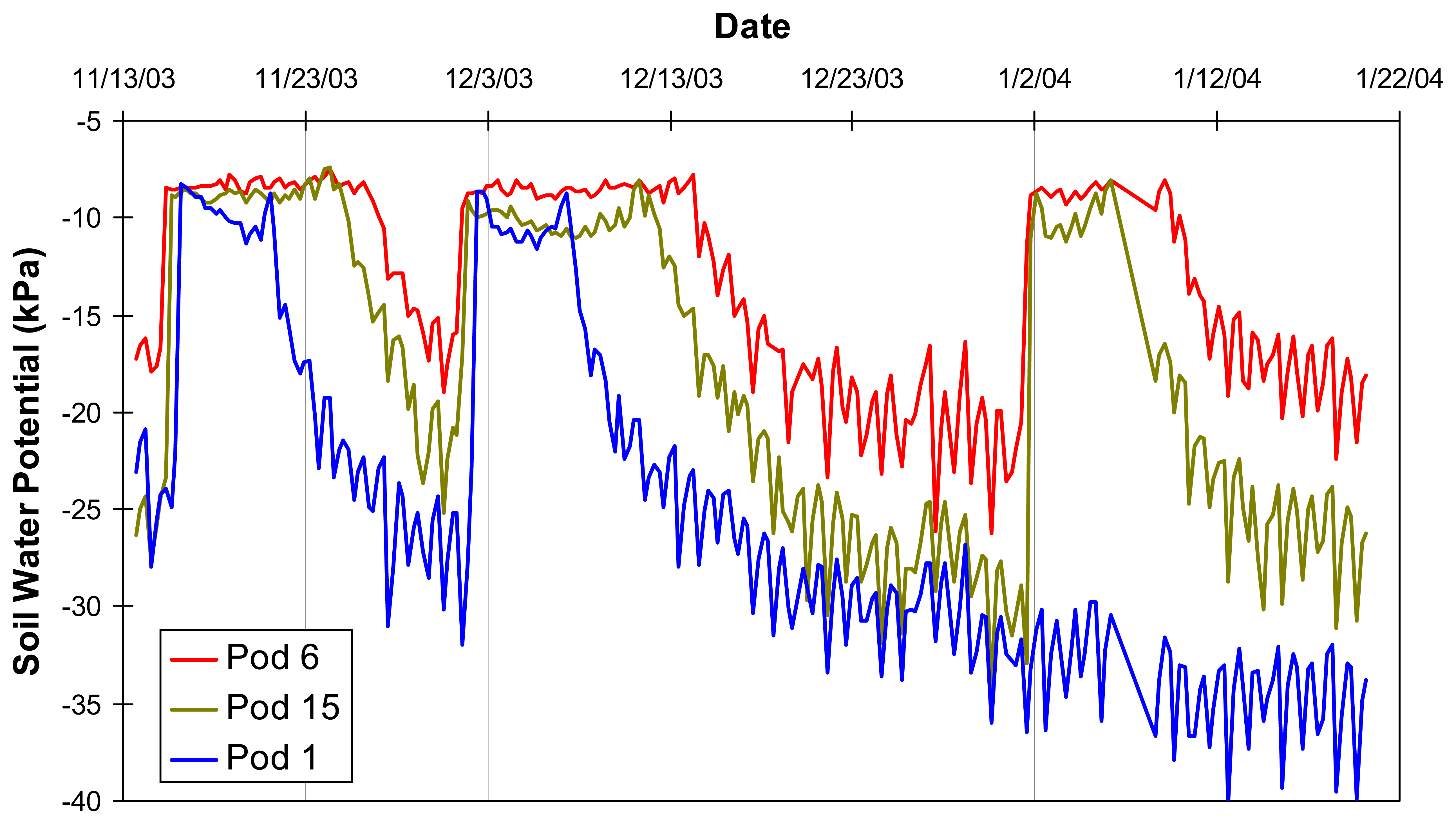
Figure 9 increases the time-scale of observation. Included now is a third flooding event occurring late on January 1, 2004. Notice, however, that this time the inflow is not left on long enough to allow the water front to reach the southern side of the basin and the soil at pod 1 continues to dry out. Figure 10 reveals that, in general, soil water potential at the surface is more responsive than that at depth. This type of subterranean measurement, the inferred vertical tracking of water movement and soil drying as a function of time, is not possible using remote measurement techniques. Coupled with the large spatial extent of the Sensor Web, this temporal vertical tracking will provide a powerful tool for understanding transient hydrologic phenomena.

These preliminary results clearly demonstrate several new methodologies for hydrology created by the Sensor Web. Both transient and subterranean hydrologic phenomena can be captured to better model and understand percolation in different soil types, and can be captured in native environments on a long-term basis. Unlike the information obtained by remote measurements, the data from the Sensor Web are continuous and not restricted by orbital paths, flight schedules, or local weather conditions. Moreover, the in-situ Sensor Web data can also be compared to remote measurements to provide ground-truth. The Sensor Web deployed in the recharge basin is therefore more than just a functioning technological test. It is a functioning scientific instrument for hydrologic use.

Summary

The primary focus of Sensor Web development thus far has been to demonstrate that the technology is stable, robust, and attractive to potential end-users. For a user community to adopt it, however, the Sensor Web needs to be more than just well-engineered; it must also be easily deployed and maintained and provide valuable output. The overall simplicity of the Sensor Web system as an operational instrument is demonstrated by the fact that most Sensor Webs are deployed and operated in a variety of environments (including Antarctica [8]) without requiring assistance from the NASA/JPL team.

As shown by our case study, the Sensor Web can provide important spatio-temporal data needed to track transient phenomena. In our hydrology example, these phenomena include flooding and infiltration. The simultaneous measurements of temperature and soil moisture at different locations and depths make it possible to monitor the changes in soil moisture in different strata. The results also provide an excellent opportunity to develop a mechanism for the study of flood dynamics in a controlled and well-instrumented environment. The Sensor Web, therefore, has a great potential to change our way of monitoring and understanding hydrologic processes on Earth and beyond. Similar examples can be found in other environmental studies.

Having demonstrated many of the Sensor Web's core capabilities with a myriad of deployments, we are now moving Sensor Web development into a new phase, focusing as much on applications as technology. The continuous, virtual monitoring and reacting capabilities have wide ranging uses for resource management, pollutant tracking, and perimeter monitoring. This step requires us to take ful advantage of the large-scale awareness already built into the Sensor Web protocols. In this way, the output of the hydrologic Sensor Web, for example, would not consist of a collection of scalar measurements (soil moisture) but rather a single vector (water motion) with pod-to-pod data fusion occurring within the Sensor Web itself. This will truly give the Sensor Web the capacity to make sophisticated, autonomous decisions. Indeed, we anticipate that future hydrologic Sensor Webs could provide early-stage triggers for satellite monitoring systems to focus on developing flood conditions and alerts for downstream communities. As awareness of this unique distributed instrument and its capabilities spreads into other user communities, the Sensor Web is expected to become an importan wireless sensor network architecture.