Airborne Chemical Sensing with Mobile Robots


1
University of Orebro, Dept. of Technology, AASS, S-70182 Orebro, Sweden
2
University of Lincoln, Dept. of Computing and Informatics, Brayford Pool, Lincoln, LN6 7TS, UK
*
Author to whom correspondence should be addressed.
Sensors 2006, 6(11), 1616-1678; https://doi.org/10.3390/s6111616
Submission received: 1 October 2006
/
Accepted: 8 November 2006
/
Published: 20 November 2006
(This article belongs to the Special Issue Gas Sensors)
Abstract
:Airborne chemical sensing with mobile robots has been an active research area since the beginning of the 1990s. This article presents a review of research work in this field, including gas distribution mapping, trail guidance, and the different subtasks of gas source localisation. Due to the difficulty of modelling gas distribution in a real world environment with currently available simulation techniques, we focus largely on experimental work and do not consider publications that are purely based on simulations.
1. Introduction
In the future when robots will be part of our daily lives in the domestic environment and at the workplace, surveillance of the ambient gas concentration could be performed by mobile robots that are equipped with an artificial sense of smell. This is especially desirable in a number of different applications in security, surveillance, humanitarian demining, and search and rescue. To endow such robotic systems with the sense of smell, gas sensing devices will need to be integrated into these robotic platforms. Among other qualities, it is expected that such gas sensors should be able to detect a variety of different odourants, demonstrate a high sensitivity to these odourants, and respond quickly and robustly in the presence of an analyte gas. In this way, a mobile olfactory robot can perform a number of olfactory related tasks which include navigating to a specific odour source, creating concentration maps of an area, and offering continuous inspection of a large area.
The value of mobile robots with an artificial sense of smell is probably most apparent in the case of gases that cannot be sensed by humans. Carbon monoxide, for example, is responsible for a large percentage of the accidental poisonings and deaths reported throughout the world each year [1, 2]. Since it is odourless, colourless and nonirritating, carbon monoxide is impossible to detect by an exposed person. It is therefore known as the silent killer [3]. Further, it has been suggested that prolonged exposure to low concentrations of carbon monoxide may have subtle adverse effects on the brain [4], typically without producing directly perceptible health effects. Accidental carbon monoxide poisoning can be caused by a fire, inadequate ventilation or obstructed furnaces. The most straightforward way to compensate for our lack of sensitivity to this gas is the installation of stationary carbon monoxide detectors. While the use of carbon monoxide alarms is certainly recommended, a stationary installation can entail problems especially when measuring low concentration levels since carbon monoxide alarms are sensitive to environmental conditions and location [1]. With respect to the dependency on the sensor location, a mobile installation has the advantage of a larger coverage and allows for an economical use of gas sensors since they are needed only once per robot instead of once for each designated location. This is particularly advantageous if several gas sensors are required to monitor other pollutants or gases that interfere with the target gas.
One should bear in mind that pollution monitoring tasks need not necessarily be performed by dedicated inspection robots. Instead, surveillance of the ambient pollutant concentration can be carried out by mobile robots that are primarily intended for other tasks. Future service robots, security robots and entertainment robots will share our habitat to a great extent. Combining their mobility with a set of suitable gas sensors presents the opportunity to monitor pollutants in a large percentage of our living space. The capability to monitor the ambient pollutant concentration will improve the value of these robots since, in addition to their other benefits, they can protect the health of their owners by attending continuously to unhealthy environmental conditions. This will naturally reduce the chance of missing places where a risk of hazardous gas was not expected.
The integration of an artificial sense of smell into mobile robotic systems is non-trivial. Investigation of the corresponding challenges has been a growing topic in robotics for the past 15 years. The technological progression of compact gas sensors is integral to the solution of detecting odours with mobile robots and much development is still needed before the gas sensors are satisfactory for real applications. Nonetheless, the integration of olfactory sensing for mobile robots has introduced a number of key research topics for mobile robotics whose investigations can progress in parallel to the sensor development. This article provides a review of these topics, which include gas distribution mapping, trail guidance, and the different subtasks of gas source localisation. It is confined to works on airborne chemical sensing with mobile robots, thus not referring to olfactory experiments with underwater robots, for example. We also do not consider publications that are purely based on simulations, since gas distribution in a real world environment is very difficult, if not impossible, to model faithfully with currently available simulation techniques.
There are already some articles that review different aspects of the field of mobile robot olfaction [5], [6], [7], and a book has been published on the subject [8]. In this article, we present a comprehensive overview that differs from the previous reviews in several ways. First, a different perspective is adopted, reflected in the structure of the presentation, that was chosen according to our conceptual separation of the different olfactory tasks. Second, we believe that accurate description of the environmental conditions under which olfactory experiments have been carried out is essential to enable meaningful comparisons between individual experiments. Therefore, special attention has been paid to describe the relevant environmental parameters as accurately as possible. We consider a thorough description of the experimental realisation to be very important, since the main components (environmental conditions, hardware design, sensing strategy and the algorithm for signal processing) cannot be studied in isolation, and often the tweaks that have to be made to an implementation are as important to the success of the implemented strategy as the underlying concept. Accordingly, this review article is considerably longer than its predecessors. Finally, it was felt that research in the field of airborne chemical sensing with mobile robots has made substantial progress during the last few years, which is understandably not reflected in earlier reviews.
1.1 Gas Source Localisation
Apart from the detection of an increased gas concentration, the task of localising a source of gas is very important. Providing robots with this ability is needed for applications such as a “smelling electronic watchman” that is able to indicate and locate dangerous gas leaks, leaking solvents or a fire at its initial stage. Assuming the existence of suitable gas sensors in the future, further possibilities could include automatic humanitarian demining [9] or localisation of the victims of an avalanche. Inspired by solutions found in biological systems, it has also been suggested to use self-produced odours to aid navigation [10, 11] and for communication with other robots [12].
Gas source localisation, however, is an intricate task under natural conditions due to the turbulent nature of gas transport, which leads to a patchy, quickly fluctuating gas distribution. The corresponding concentration field does not guide the way to its source by means of a smooth concentration gradient and does not necessarily indicate the source location by a maximum of the instantaneous concentration distribution (see Section 3). While the gas source localisation problem is very challenging, it nonetheless deserves study since it is the key to many significant applications. In addition, investigating gas source localisation strategies can be expected to lead to a deeper understanding of the physical properties of turbulent motion, as well as the way in which animals use odours for navigation purposes.
1.2 Gas Source Localisation Taxonomy
The gas source localisation problem can be broken down into three subtasks [13]:
- gas finding - detecting an increased concentration of a target gas,
- gas source tracing*- following the cues determined from the sensed gas distribution (and eventually using other sensor modalities) towards the source,
- gas source declaration - determining the certainty that the source has been found.
This classification follows a suggestion of Hayes et al. [14], with the difference that the existence of a sufficiently strong and constant airflow is not presumed. Such conditions allow the identification of a plume from the gas distribution which can be followed to its origin. The term “plume” refers to an aerial trail of gas which has a shape that resembles the shape of a feather [15]. However, a discernible gas plume can not be guaranteed, for example, in an unventilated indoor environment.
The introduced taxonomy provides a useful conceptual framework for classifying gas source localisation strategies, but approaches do not have to address the subtasks independently. An example could be a set of reactive behaviours that causes the robot to explore a certain area as long as no increased concentration is detected and moves the robot closer to the gas source if the sensed concentration exceeds a certain threshold. Such a set of behaviours can address both subtasks, gas finding and gas source tracing, without it being possible to associate each subtask with a separate subset of behaviours. It should also be noted that a complete gas source localisation strategy does not necessarily involve some sort of source tracing if it implies a means of deducing the location of the gas source from a distance.
It should be emphasised that suggestions for gas source localisation may not rely only on gas sensor measurements. Temperature or humidity sensors can provide additional cues to localise certain types of gas sources. In the case of a reasonably unidirectional airflow, the local upwind direction can serve as an estimate of the direction to the gas source. Air flow measurements can further be used for more efficient gas finding and gas source declaration strategies, and a vision system might indicate candidate objects for subsequent investigation using a gas source declaration strategy.
1.3 Gas Finding
While most of the publications in the field of airborne chemical sensing with mobile robots are concerned with gas source tracing, little attention has been paid so far to gas finding and gas source declaration. Solutions to these problems are required in addition to gas source tracing strategies in order to provide a complete solution to the gas source localisation problem. However, they are also important in other contexts, for instance when only the presence of a gas source has to be detected (gas finding) or when the task is confined to determining whether a given object is a gas source or not (gas source declaration).
An appropriate gas finding strategy is sufficient for surveillance applications where a mobile robot is only supposed to trigger a general warning when detecting a specific gas, without providing more detailed information. Apart from a suitable sensor set-up, the problem of gas finding requires mainly to select an appropriate exploration strategy and to define a threshold value above which the target gas is assumed to be present. Generally, this threshold value needs to be adaptive to compensate for varying environmental conditions or sensor drift, for example. A suitable exploration strategy for gas finding has to take into account the additional complexity that a simple sequential search is not guaranteed to succeed due to the stochastic nature of the plume [16].
1.4 Gas Source Declaration
The fundamental problem for gas source declaration using only the sense of smell is to find regularities in a turbulent concentration distribution which make it possible to decide whether a certain area contains a gas source or not. The most straightforward feature to look for is a local concentration maximum. In order to derive a meanigful indicator for gas source declaration, the time-averaged concentration distribution has to be considered. Searching for maxima in the instantaneous concentration field is of little help since they are often found far away from a source. Whether a turbulent gas distribution provides further regularities that allow for reliable gas source declaration is an exciting question that cannot be answered conclusively at the moment. It is very difficult to derive the general features required in the turbulent fine structure from the equations that describe turbulent gas spread and it is possible that the bandwidth of commonly used gas sensors might not be sufficient to resolve these features.
Using wind sensors in addition to gas sensors can be helpful in the context of gas source declaration if the airflow is strong enough to be measured reliably. In this case a correlation between airflow direction and the measured concentration can be used to declare a gas source, for example, by determining a drop between the concentration measured in downwind and upwind direction.
Having a reliable gas source declaration strategy can be sufficient to address gas source localisation even if the full problem cannot be accomplished using gas and wind sensors only. An object could first be located using other sensor modalities (a vision system, for example), and then classified using the gas source declaration method. Such a procedure assumes that candidate gas sources can be perceived with the additional sensor modality. Assuming the availability of sufficiently sensitive gas sensors, possible applications include the identification of suspicious items containing illegal narcotics or explosive materials, and employment in rescue robots to determine whether a victim is still alive by measuring their carbon dioxide output.
1.5 Gas Distribution Mapping
Another issue that has not yet been considered extensively is gas distribution mapping. In addition to the temporally fluctuating character of turbulent gas transport, it has to be taken into account that chemical gas sensors only provide information about the small volume of gas that their surface interacts with. It is therefore impossible to measure the instantaneous concentration field without using a dense grid of sensors. However, it is often sufficient to know the time-constant structure of a gas distribution. This might even be more important than knowing the exact location of gas sources, for example, because it allows to determine areas in which high concentrations of a harmful gas are to be expected. Mobile robots that are able to map the gas distribution in a contaminated area could be used in rescue missions by incident planning staff to prevent rescue workers from being harmed or killed by explosions, asphyxiation or toxication [17]. Other applications for gas distribution mapping include air quality monitoring and surveillance of pedestrian areas in cities, and precision farming [18], where the average distribution of particular gases could be used as a non-intrusive way of assessing the soil condition or the status of plant growth to enable a more efficient usage of fertiliser.
Creating a map of the average concentration of a target gas also provides a means of addressing the gas source localisation problem. However, this approach has some drawbacks. First, it is required that the environmental conditions and the activity of the gas source do not change drastically within the time frame of the mapping process. Second, gas source localisation methods based on gas distribution mapping can be slow due to the time it takes to build a reliable representation of the average concentration in which turbulent fluctuations are sufficiently “averaged out”. On the other hand, the time consumption scales down with the number of robots utilised with a lower bound that is theoretically given by the time required to compensate for turbulent fluctuations with a dense grid of sensors. A further advantage is that the information about the concentration distribution in the whole inspected area may be used to increase the accuracy and the certainty of the gas source location estimate.
1.6 Outline
The rest of this article is structured as follows. First, a brief summary of gas sensor types that have been used with mobile robots, is given in Section 2. Next, the peculiarities of machine olfaction in a natural environment are discussed in Section 3. Then, an overview of early work on gas-sensitive robots is given in Section 4, followed by a classification of literature in the field of airborne chemical sensing with mobile robots in Section 5. Using this classification as a guideline, the following sections review approaches to gas distribution mapping (Section 6) and trail following (Section 7), suggestions for gas finding (Section 8), work on gas source tracing with and without the assumption of a strong constant airflow (Sections 9, 10, and 11), and approaches to the full gas source localisation problem based on analytical models (Section 12). Finally, an overview of the work on gas source declaration is provided (Section 13) followed by conclusions and and a discussion of open questions (Section 14).
2. Gas Sensors and Electronic Noses
During the 1980s research on machine olfaction boomed [19–22] leading to a generally accepted definition of an electronic nose [23] as an instrument that comprises an array of heterogeneous electrochemical gas sensors with partial specificity and a pattern recognition system [24]. Probably the first report of a similar device was published by Moncrieff at the beginning of the 1960s [25]. Gas sensors are devices that measure the ambient gas atmosphere based on the general principle that changes in the gaseous atmosphere alter the sensor properties in a characteristic way. A variety of different sensor types have been developed beginning with early work by Hartman, Wilkens and Sauerbrey [26–28], though mainly conductivity sensors have been used in connection with mobile robots. These sensors operate on the principle of measuring a relative resistance change between two electrodes. Different kinds of sensing material can be deposited on these electrodes whose properties change upon interaction with a gas. Three types of materials in particular are commonly used: metal oxides, conducting polymer composites and intrinsically conducting polymers. The operating mechanism for each type of sensing material is briefly described below. Apart from conductivity sensors, gas detection has been done using optical sensors, surface acoustic wave sensors, gas sensitive field effect transistors and quartz microbalance (QMB) sensors. Of this list, QMB sensors show the most promise for mobile robot applications and recent improvements to this sensor are also described.
2.1 Metal Oxide Gas Sensors (MOX)
Metal oxide (MOX) gas sensors are composed by depositing a metal oxide film onto a substrate made of glass, silicon alumina or some other ceramic. Platinum, silver or aluminium electrodes are also deposited onto the substrate and a heating element is printed on the back. A voltage across the heated surface causes an electrical current through the grain boundaries of the sintered polycrystalline surface of the semiconductor. Absorption of oxygen at the sensor surface increases the potential barrier between the grain boundaries, which causes a large effect on the sensor's resistance [29]. The conductivity of the device thus sensitively reflects the rate of redox reactions with the ambient gas. The most common metal oxide sensor is the n-type, which uses a (SnO2) semiconductor. In the n-type sensor, analyte gas is sensed by its effect on the electrical resistance, which decreases in the presence of reducing gases [29, 30].
The sensitivity of the metal oxide sensor depends on a number of factors. Thinner film thickness has been shown to improve sensitivity with thin films ranging from 6 - 1000 nm compared to 10 to 300μm for thick films [31]. The addition of a catalytic metal to the oxide such as Cu has been shown to increase sensitivity to certain gases (although excessive doping can reduce sensitivity) [30]. Also, the sensitivity of the metal oxide can vary depending on the operating temperature. High temperatures ranging from 250°C to 500°C are required for proper operation [29].
The advantages that have made MOX sensors the most widely used gas sensor in mobile robotic applications are their high sensitivity (down to the sub-ppm level for some gases), the usable life-span of three to five years, and the comparatively low susceptibility to changing environmental conditions. Thin film metal oxide sensors are small and relatively inexpensive to fabricate, and can be integrated directly into the measurement circuitry. However, as a consequence of the high operating temperature, MOX sensors consume comparatively much power. In addition, the sensors typically have to be heated for 30 to 60 minutes before they can be used. Other disadvantages are the variance of the response characteristics between individual sensors, the slow recovery after the target gas is removed (15 to 70 seconds [32]), the weak durability over a prolonged time [33], and the poor selectivity. Although it is possible to a certain extent to control the sensitivity for a particular target gas by using different sensor preparation methods and a varying operation temperature [34], the combustion process is generally not strongly selective to the precise structural details of the gas molecules. Furthermore, the sensors suffer from sulphur poisoning due to irreversible binding of compounds that contain sulphur to the sensor oxide [35], and ethanol can also blind the sensor from other volatile organic compound gases [31].
2.2 Conducting Polymer Gas Sensors
Conducting polymer (CP) sensors have been used in the first commercial electronic nose devices. As in the case of MOX sensors, the measurand of conducting polymer sensors is the resistance of the surface layer. Instead of a semiconductor, a thin polymer film is used, which is usually deposited across the gap between two gold electrodes by electrochemical polymerisation. The vapour-induced expansion of the polymer composite causes an increase in the electrical resistance [36]. As a result, the response of the sensor depends largely on the rate of diffusion of the vapour into the polymer and can vary between several seconds to several minutes [37].
Two types of conducting polymer sensors are available for odour detection: doped (intrinsic) and composite (extrinsic). In both sensor types common monomers used for fabrication include pyrrole, indole, aniline and thiophene. The difference with the composite conducting polymers is the combination with conductive polymers or fillers (carbon black) which thereby increases conductivity [32]. It was shown in [38] that composite conducting polymers sensors gave higher sensitivity, and greater reproducibility than the doped CP in initial experiments.
Generally, conducting polymer sensors are comparatively easy to prepare (although the conditions have to be carefully controlled and the chemicals have to be suitably purified in order to achieve reproducible results) and a wide range of materials with a varying sensitivity for different organic gases can be synthesised. In contrast to the MOX sensors, conducting polymers can operate at room temperature, therefore power consumption is low. Other advantages include high discrimination in an array of sensors, operation in conditions of high relative humidity and linear responses for a wide range of gases [36]. On the other hand, the actual level of sensitivity is approximately one order of magnitude lower than that of metal oxide sensors. Further disadvantages are the effects of aging, which manifests in sensor drift, and a poor understanding of the mechanism behind the conducting polymers.
2.3 Quartz Microbalance Sensors (QMB)
Acoustic wave gas sensors comprise a piezoelectronic substrate, usually quartz, and a coating with a specific affinity. By using different coatings the device can be made responsive to different gases. During operation, an alternating electric field is applied to generate an elastic wave in the quartz crystal. Temporarily absorbed molecules perturb the propagation of the acoustic waves due to the effect of the added mass and by changing the viscoelastic properties of the coating layer. The resulting shift of the fundamental frequency of the quartz crystal is then measured as the output of the sensor.
Acoustic wave gas sensors are also known as quartz crystal microbalance (QMB or QCM) because the device can be regarded as a balance that is highly sensitive to the weight of gas molecules. Depending on whether the effect of surface waves or bulk waves is utilised, these sensors are also referred to as SAW or BAW devices.
Acoustic wave gas sensors can offer rapid response (typically 10s [39]). In particular, the time required for recovery is usually shorter compared to metal oxide gas sensors. Further advantages of the QMB sensor technology are the low power consumption, the possibility to control the selectivity over a wide range, long term stability and a long lifetime. On the other hand, standard QMB sensors exhibit a comparatively low sensitivity to the target gas and have a limited robustness to variations in humidity. Other disadvantages include a complex fabrication processes and poor signal to noise performance due to surface interferences and the size of the crystal [37, 40].
A better sensitivity can be achieved by operating QMB sensors at a higher frequency since the sensitivity scales with the square of the fundamental frequency according to the simple standard model by Sauerbrey [27]. For standard QMB sensors, however, the minimal thickness at which a quartz disk is still mechanically stable corresponds to a maximum fundamental frequency of approximately 30 MHz. Typical QMB sensors use resonance frequencies of 10 MHz [31]. A promising development here concerns the so-called High Frequency Fundamental (HFF) Quartz crystals introduced by Kreutz et al. [41]. By etching a small circle in the middle of a regular 10 MHz quartz crystal, much higher frequencies of 50 MHz and more can be achieved at the inner circle while the thicker outer ring maintains the mechanical stability. First results of Kreutz et al. using an HFF-QMB sensor with a fundamental frequency of 51.84 MHz show an increase in signal intensity by a factor of 11.5 [41], which is lower than the boost expected with the simple standard model by Sauerbrey but nevertheless indicates the potential of this technique.
3. Gas Sensing in a Natural Environment
Electronic noses have been studied extensively under laboratory conditions. Numerous publications are available, for example, in the field of food analysis. To name only a few, this includes tests on the freshness of fish [42], quality estimation of ground meat [43], recognition of illegally produced spirituous beverages [44] and discrimination of different coffee brands [45].
These results cannot be obtained in the same manner when using a mobile robot due to the influence of varying environmental conditions and restrictions because of limited resources such as power and the available space, for example. An important aspect that is difficult to transfer to a mobile system is the sample handling process. In most laboratory-based applications (see Fig. 1 for example) much effort is expended to prepare the volatile components before they are analysed with the gas sensor system. Typically headspace samplers are used, which prepare a defined sample of evaporated material (the so-called headspace) and deliver the sample in a well defined way to a chamber that contains the gas sensors [46]. Moreover, best performance was achieved in laboratory experiments by using a measurement technique that requires a second gas (e.g. clean air with known humidity), which is periodically routed to the sensor chamber. It serves as the carrier gas for the headspace sample and as a reference for tracking the baseline level of the sensor response. Due to the demand for real-time operation and restrictions of weight, space and power consumption it is usually not feasible to establish the same sophisticated sample handling process on a mobile robot.
As a consequence of the limited resources it is also difficult to achieve sufficiently stable environmental conditions. Gardner and Bartlett report typical accuracies of ±0.1°C temperature, ±1% relative humidity and ±1% flow rate as important conditions when employing electronic nose technology [24]. For application on a mobile robot, larger variations in the environmental conditions have to be tolerated. Consequently, research in the field of airborne chemical sensing with mobile robots has focussed so far mostly on using gas sensors for detection of a known target gas and localisation of the gas source rather than discrimination of different gases. To avoid confusion, a complete gas-sensitive system used on a mobile robot is sometimes referred to as a “mobile nose” [47].
3.1 Gas Distribution in a Natural Environment
A major problem for gas source localisation in a natural environment is the strong influence of turbulence on the distribution of gas. Turbulent transport generally dominates the dispersal of gas due to molecular diffusion. For example, the diffusion constant of gaseous ethanol at 25°C and 1 atm is D = 0.119 cm2/s, corresponding to a diffusion velocity of 20.7 cm/h [48]. Apart from very small distances where turbulence is not effective and diffusion can be distinct along steep concentration gradients, molecular diffusion can thus be discounted as a major factor concerning the spread of gas.
Turbulent flow exhibits several general characteristics described below (following the summary by Roberts and Webster in [50]). First, turbulent flow is unpredictable. Turbulence is chaotic in the sense that the instantaneous velocity (and consequently also the instantaneous concentration of a target gas) at some instant of time is insufficient to predict the velocity a short time later.
Second, as mentioned above, turbulent transport is considerably faster than molecular diffusion. This is indicated in Fig. 2, which shows colour-coded concentration distribution in simulated gas mixing due to the effect of diffusion alone (bottom, left) and due to diffusion and turbulence (bottom, right). The pictures in the lower part of the figure show snapshots of the gas distribution that evolved from the circular distribution depicted in the upper part. These distributions were obtained by Smyth and Moum by means of a numerical solution of the equations of motion [49]. It is apparent from the figure that turbulent flow causes a much quicker spreading of the target gas. As an average effect this can be modelled by defining an effective turbulent diffusion coefficient (the eddy diffusivity, see for example [51]).
Third, a turbulent flow comprises at any instant a high degree of vortical motion. These continuously fluctuating eddies range in size from the largest geometrically bounded scales of the flow (the so-called integral length) down to the scales where only molecular diffusion is effective (Kolmogorov microscale). While large scale eddies cause a meandering dispersal, small scale eddies stretch and twist the gas distribution, resulting in a complicated patchy structure (see Fig. 2). The instantaneous distribution exhibits no smooth concentration gradients that indicate the direction towards the centre of the gas source. Assuming reasonably stable conditions such as uniform and steady flow, however, the time-averaged concentration field varies smoothly in space with moderate concentration gradients.
A fourth characteristic of turbulence is the dissipation of kinetic energy. Turbulent kinetic energy is passed down from the largest eddies to the smallest, where it is finally dissipated into heat by viscous forces (this is called the energy cascade). The magnitude of the viscous forces determines the minimal eddy size (Kolmogorov microscale, see [8, 50] for details).
Another important transport mechanism for gases occurs due to the fluid flow itself (advective transport). This mechanism is typically effective even in an indoor environment without ventilation due to the fact that weak air currents exist as a result of pressure (draught) and temperature inhomogeneities (convection flow).
In summary, the instantaneous concentration field of a target gas released from a static source is a fluctuating typically asymmetrically shifted distribution of intermittent patches of high concentration with steep gradients at their edges. These properties are illustrated in Fig. 3, which shows typical sensor readings in the vicinity of a gas source (evaporating liquid ethanol). In this experiment taken from [52], the robot passed the source along a straight line at a low speed of 0.25 cm/s in order to measure the distribution of the analyte gas accurately. Despite the smoothing effect due to the slow recovery of the metal oxide gas sensors used, the curve in Fig. 3 reveals the existence of many local concentration maxima. Moreover, the absolute maximum was found approximately 70 cm away from the actual location of the gas source. It is a very typical result that the location of the gas source and the absolute maximum do not coincide if the gas source has been active for some time (naturally, if the gas source has just been “opened”, the highest concentration must occur close to the surface or the outlet of the source). On one hand, this can be attributed to the fact that even for a gas sensor which is located directly over or under the gas source, the molecules of the analyte gas have to travel some distance to reach this sensor if it is not mounted level with the gas source. On the other hand, it is also a consequence of the fairly constant concentration in isolated gas patches which changes slowly with time – and therefore also with spatial distance from the source – and does not depend strongly on the average concentration. In the case of turbulent diffusion from a small source, the peak concentration values are generally an order of magnitude higher compared to the time-averaged values [50].
4. Early Work on Airborne Chemical Sensing with Mobile Robots
Chemical sensing entered the field of mobile robotics in the beginning of the 1990s. Early work focused on the use of gradient-following (chemo-tropotaxis) for gas source tracing without an explicit description of the environmental conditions. Rozas et al. report on a preliminary experiment with a mobile robot where a decreasing concentration was observed as the distance to the gas source was increased [53]. This result was found by measurements with a ventilated gas capture device (containing six metal oxide sensors) mounted on a mobile robot. The measurements were performed at four different distances from the source (0 m, 0.5 m, 1 m and 3 m, respectively). Only one trial is reported for each of the three analytes tested, making the reproducibility of the results unclear. Due to the turbulent character of gas propagation, however, a monotonic relationship between the observed concentration and the distance to the source cannot be expected in general.
Sandini et al. considered the problem of gas source tracing as an example of a localisation task, which has to be performed based on local information that does not directly indicate the source location [54]. As a possible solution, the authors suggest a strategy that involves periods of random exploration and gradient following, and the robot switches between these states depending on whether the gas sensor output is above or below a certain threshold. Gradient following was implemented by applying a positive or negative driving command depending on the sign of the concentration gradient sensed with a pair of metal oxide sensors. The authors point out a notable limitation for gradient-following strategies based on chemical sensor measurements: that the instantaneous concentration gradient might not be accessible because of the implicit temporal integration performed by the sensors due to their long decay time. However, quantitative results of their gas source tracing experiments are not given, and the environmental conditions are not specified in sufficient detail to permit meaningful comparison with similar experiments.
5. Classification of Literature on Airborne Chemical Sensing with Mobile Robots
The majority of the subsequent publications in the field of airborne chemical sensing with a mobile robot contain a description of the environmental conditions. The following sections provide a review of these publications, which basically address three problem domains: gas distribution mapping, trail guidance, and gas source localisation. The literature review is organized according to the classification scheme shown in Fig. 4 where, on the left side, the problem domains are indicated, and, on the right side, the number of the corresponding section in this article. It can be seen from Fig. 4 that most work deals with the problem of gas source localisation in some way.
The publications on gas source localisation can be divided into the subtasks of gas finding, source tracing and source declaration. A further distinction can be made between gas source localisation methods that depend on information about the local wind vector and methods that do not rely on wind measurements. Despite the improved sensitivity of anemometers it is still hard to measure wind speed accurately on a mobile robot in a typical indoor scenario. In an industrial or domestic indoor environment with moderate ventilation, wind fields with velocities less than 5 cm/s are typically encountered [6, 55]. Due to turbulent fluctuations, the wind velocity will be at least intermittently below the sensitivity threshold of state-of-the-art anemometers. In the absence of ventilation the wind velocities will be even lower and therefore more difficult to measure. A further complication arises from the motion of the mobile robot that carries the wind sensor. The faster the robot moves, the stronger will be the influence of the airstream caused by its own motion. With increasing speed of the robot it thus becomes increasingly difficult to break down the measured wind vector into a component caused by the environmental airflow and a component caused by the robot motion. Consequently, it is reasonable to differentiate between methods which require that the local wind vector can be sensed reliably and methods which do not rely on the local wind vector.
6. Gas Distribution Mapping
6.1 Simultaneous Measurements With Multiple Stationary Sensors
A straightforward method to create a representation of the time-averaged concentration field is to perform concentration measurements† over a prolonged time with a grid of gas sensors. The gas sensor locations can be chosen such that the average concentration values can be represented straightforwardly in a grid map with cells that reflect the arrangement of the gas sensors.
Ishida and co-workers used partially simultaneous measurements to characterise the gas distribution in the experimental environment on various occasions, typically with four or eight sensors and an average time of between 5 and 8 minutes [56]. A gas distribution map created in this way (concentration measurements at 33 grid points, averaged over 5 minutes) is shown in [57], for example. A similar method was applied in [58], but instead of the average concentration, the peak concentration observed during a sampling period of 20 s was used to create the map. Of course, it would be misleading to think of the resulting representation as a concentration map. However, there is evidence that the peak concentration might be a better indicator of proximity to a gas source compared to the average concentration [58]. Thus, if considered instead as a gas distribution map, a representation based on peak concentrations may be a preferable solution, especially with regard to short sampling intervals. Different indicators of gas source proximity are discussed in Section 13.3.
Creating a gas distribution map from simultaneous measurements with multiple stationary sensors has the advantage of reduced time consumption but requires calibration to match the sensitivities of the sensors. With an increasing area, establishing a dense grid of gas sensors would also involve an arbitrarily high number of fixed gas sensors, which poses problems such as cost and a lack of flexibility. Furthermore, a dense array of metal oxide sensors (as used in [57], for example) can cause a severe disturbance due to the convective flow created by the heaters built into these sensors [59].
6.2 Bi-Cubic Interpolation Map From Stationary Sensor Response
Instead of using a grid of gas sensors, concentration measurements can be also performed in succession in the case of uniform delivery and removal of the analyte gas and stable environmental conditions. Consecutive measurements with a single sensor and time-averaging over 2 minutes for each sensor location were used by Pyk et al. [60] to create a map of the distribution of ethanol from an active and uniform gas source in a wind tunnel with an airflow of 0.67 m/s. Fig. 5, left shows the time-averaged response obtained in this way with a gas sensor array placed at 63 equally spaced locations. In between the measurement locations, the map was interpolated using bi-cubic filtering.
6.3 Triangle-Based Cubic Interpolation Map From Dynamic Response
Fig. 5, middle and Fig. 5, right show a gas distribution map obtained from the response of a gas sensor array carried by a mobile robot, which was driven on a zig-zag trajectory at a translational speed of approximately 10 cm/s. While Fig. 5, middle shows the result of a single run, Fig. 5, right was obtained by averaging over three runs. The trace of the robot is indicated by dashed lines. Since the measurement locations are not equally distributed in this case, triangle-based cubic filtering was used for interpolation. The gas distribution maps in Fig. 5 indicate a plume-like structure and reveal high concentrations in the vicinity of the gas source placed at (x,y) = (0 m, 1.5 m). The dynamic response interpolation map in Fig. 5, middle roughly resembles the map obtained from stationary sensor response in Fig. 5, left but shows a more jagged distribution. This indicates a flaw of interpolation-based mapping methods. The response values represented in the map are either obtained directly from the acquired sensor value at locations where a measurement was taken or by interpolation in between these locations. Therefore, there is no means of “averaging out” instantaneous response fluctuations at measurement locations. Even if response values were measured very close to each other, they will appear independently in the gas distribution map with interpolated values in between. Consequently, the dynamic response interpolation map obtained by averaging over three runs in Fig. 5, right looks even more jagged than the map created from a single run in Fig. 5, middle.
6.4 Odour Hits Histogram Map From Dynamic Response
Gas sensor measurements acquired with a group of simultaneously operating mobile robots were used by Hayes et al. to create a representation of the gas distribution using a two-dimensional histogram [16]. The histogram bins contain the accumulated number of “odour hits” received by all robots in the corresponding area while they performed a random walk behaviour. Odour hits are counted whenever the response level of the gas sensors exceeds a defined threshold. An example of such an “odour hits histogram” is shown in Fig. 6. This gas distribution map was recorded with six robots while performing a random walk behaviour for one hour in a 6.7 × 6.7 m2 arena. The source was a hot water pan located in one corner of the arena and several fans mounted behind the pan created an airflow with an average speed of approximately 1 m/s. Each robot was equipped with a single conducting polymer sensor to measure water vapour. The advantage of this set-up is that the conducting polymer sensors provide a very fast response time in the order of 100 ms.
In addition to the dependency of the gas distribution map on the selected threshold, a problem with using only binary information from the gas sensors is that much useful information about fine gradations in the average concentration is discarded. A further disadvantage of this method is that it requires perfectly even coverage of the inspected area by the mobile robots. It remains to be investigated how well the suggested approach can be transferred to a system with a substantially longer response time (where a sequence of response peaks arriving in short succession may be detected as one odour hit) and to which extent an odour hits histogram corresponds to the average concentration field. Naturally, it takes a comparatively long time to obtain statistically reliable results and this time scales up quadratically with the dimension of the arena if the number of robots is not increased accordingly. Suitable extrapolation on the measurements can reduce the time to build a gas distribution map while preserving the same level of detail. In the above approach there is no extrapolation on the measurements apart from the quantisation into histogram bins.
6.5 Kernel Extrapolation Gas Distribution Gridmap From Dynamic Response
A method to create gas distribution gridmaps with kernel-based extrapolation on gas sensor readings collected by a mobile robot was introduced by Lilienthal and Duckett [61]. The mapping algorithm creates a representation that stores belief about the average relative response of gas sensors in a grid structure corresponding to a map of the average relative concentration of a detected gas. Gas sensors provide information about the reactions at their surface, which typically cover only a small area in the order of 1cm2. In order to compensate for the small overlap between single measurements, spatial integration of the point measurements is carried out by convolving sensor readings with a Gaussian kernel to extrapolate on the measurements. The kernel can be seen as modelling the information content of a given measurement about the average concentration distribution with respect to the point of measurement. This information content decreases with increasing distance to the point of measurement. Note also the analogy of this mapping approach with the problem of estimating density functions using a Parzen window method [62]. It can be shown that for continuous density functions, the Parzen window estimate converges to the true density function regardless of the window function if the number of samples approaches infinity and the window function is well-behaved [63]. This condition is satisfied for a variety of window functions, including Gaussian kernels. Accordingly, a kernel-based extrapolation method to map gas distribution can be regarded as a refinement of a histogram-based approach.
Some examples of kernel-extrapolated gas distribution gridmaps calculated from the response of two metal-oxide gas sensor arrays carried by a mobile robot are shown in Fig. 7. The obtained gas distribution maps can represent fine gradations of the average concentration. The algorithm also does not depend on a perfectly even coverage of the inspected area and can cope to a certain degree with the temporal and spatial integration of successive readings that metal-oxide gas sensors perform implicitly due to their slow response and long recovery time [52]. It is necessary, of course, that the trajectory roughly covers the available space. In order to obtain a faithful representation of gas distribution despite the slow sensor dynamics (“memory effect”), the robot's path also needs to fulfill the requirement that the directional component of the distortion due to the memory effect is averaged out. This can either be achieved approximately by random exploration or in a strict manner by using a predefined path where the robot passes each point in the trajectory equally often from opposite directions. If the trajectory of the robot fulfills this requirement, the time-constant structures of the gas distribution will be represented faithfully in the gridmap, being slightly expanded and blurred but not shifted. The accuracy of the gridmaps produced by the kernel-based extrapolation algorithm therefore degrades gracefully with respect to the ratio between the time constant of the sensor dynamics and the speed of the robot (i.e. the slow sensor dynamics). The algorithm introduces the kernel width σ as a selectable parameter, corresponding to the size of the region of extrapolation around each measurement. This parameter allows the user to decide between a faster or more accurate map building process. Its value has to be set large enough to obtain sufficient coverage according to the path of the robot. Conversely, this means that for a larger kernel width a faster convergence can be achieved while preserving less detail of the gas distribtuion in the map. Consequently, the selected value of the kernel width σ represents a trade-off between the need for sufficient coverage and the aim to preserve fine details of the mapped structures. Parameter selection and the impact of sensor dynamics are discussed in more detail in [52].
As with all of the mapping algorithms discussed in this section, the kernel-based extrapolation algorithm can only represent time-constant structures in the gas distribution. Also the effort (either in terms of time consumption or the number of sensors) to converge to a stable representation, scales quadratically with the size of the environment. The convergence time of the kernel-based extrapolation algorithm was found to be in the range of 10 to 30 minutes in an extensive set of gas distribution mapping trials with a total duration of almost 70 hours. In this experiment, a single robot was driven at a speed of 0.05 m/s, and had to cover an area of 6 m2 to 14 m2. The kernel width was 0.15 m. Further details are given in [52, 64]. A convergence time of 10 to 30 minutes is considerably higher than the lower limit due to the physics of the problem, which is expected to be in the order of a few minutes. A mapping algorithm can achieve convergence at this time-scale only if a sufficiently high number of gas sensors are used simultaneously. How the convergence time of kernel-extrapolation gas distribution gridmaps is affected by the number of robots, however. can not be decided from the experiments that are available so far.
6.6 Model-Based Gas Distribution Mapping
Any approach that assumes a particular gas distribution model and provides an estimation of the corresponding parameters can also be considered as a method for gas distribution mapping. Model-based approaches have the advantage that it can be sufficient to explore just a small fraction of the space to estimate the parameters of the model, and that map creation can be very fast. On the downside, model-based approaches to gas distribution mapping rely on well-calibrated gas sensors and an established understanding of the interaction between gas sensors and the environment, which also means that all parameters of this interaction must be known. Further they depend crucially on the underlying model. Complex numerical models based on fluid dynamics simulations are computationally expensive and depend sensitively on accurate knowledge of the state of the environment (boundary conditions), which is not available in practical situations. Simpler analytical models, on the other hand, often rest on rather unrealistic assumptions and are of course only applicable for situations in which the model assumptions hold at least approximately. Since model-based approaches typically include the position of the gas source as a parameter, they can be used for gas source location. Accordingly, some model-based approaches are discussed in more detail in Section 12.
6.7 Performance Evaluation of Gas Distribution Mapping Algorithms
The evaluation of the performance of a gas distribution mapping algorithm remains a challenging problem since it is difficult to identify the ground truth in this domain. A straightforward possibility would be to measure the gas distribution simultaneously with a grid of gas sensors (ground truth) and a mobile robot. It has not been done so far, however, partly due to the problem that the mobile robot could collide with stationary sensors placed at the same height as the sensors of the robot. The same approach would be easier to implement with a grid of gas sensors placed at a different height but then it is not clear whether this could still serve as an adequate ground truth for a two-dimensional gas distribution map created at the height of the robots' gas sensors.
Despite the mentioned problems, it can be expected that identifying a notion of the ground truth with independent concentration measurements has the potential to improve our understanding of the gas distribution mapping process. All the gas distribution mapping approaches suggested so far have been restricted to a two-dimensional representation. Another promising direction for future work is therefore to investigate three-dimensional gas distribution mapping.
7. Trail Guidance
Olfactory markings are often used by animals to store and communicate spatial information. A well-known example concerns ants that mark the path to a source of food with an odour trail [65]. Because the information is stored physically in the environment, there is no need for a sophisticated representation of the environment in the animal's brain. By means of varying the intensity and frequency of the trail marking, additional information can be communicated such as the quality to which the food trails leads. Chemical markings are also particularly suited to encoding temporal information due to their naturally fading intensity. Ants exploit this property of pheromone communication when they indicate the “popularity” of the corresponding path simply by refreshing the odour trail they are following.
Chemical markings are of possible benefit for a number of applications in the field of mobile robotics. Olfactory trails could provide an inexpensive and more flexible alternative to the metal wires buried under the floor that are often used by industrial automated guided vehicles (AGV) [66]. Apart from establishing a path to follow, odour trails could also be used in order to provide a temporary repellent marking, indicating areas of the floor that have been cleaned, for example [10, 67]. While this would be particularly beneficial to coordinate the behaviour of multiple robots, it could also be helpful in the case of a single robot, because it avoids the necessity for maintaining a consistent spatial representation. Further application scenarios of trail guidance for mobile robotics are discussed by Russell in [11].
7.1 Air Curtain Technique
In contrast to the task of localisation of a distant gas source, the impact of turbulence is considerably reduced in the case of trail guidance because of the low sensor-to-source distance, which was often in the order of 10 mm in the experimental work published in this area. Odour trails placed on the floor are covered by a layer where the airflow is laminar. This layer is so thin that current robots cannot measure concentrations in this region [69]. However, compared with experiments in which a distant source is to be localised, the proximity of the sensors to the trail causes a much stronger differentiation of the average concentration gradient in the sensor signal. Furthermore it has been argued that it is possible to increase the differentiation near the floor by introducing well adjusted additional airflows to block external ones, thus establishing an “air curtain” [68] as indicated in Fig. 8. Recently, there have been conflicting reports on the usefulness of the air curtain technique. Larionova et al. report on their observation that the boundary of an area marked with an alcoholic cleaning solution could be found less reliably when using an air curtain set-up [67]. Consequently, they disposed of the fans creating the air curtain used in earlier work [70] and returned to a system that uses a plain vacuum pumped gas sensor. Currently it is unclear whether the different appraisals of the air curtain technique are due to small differences in its implementation or due to the different tasks considered: detecting a chemically marked narrow trail [68] or a comparatively wide area [67].
7.2 Trail Guidance Strategies Assuming a Pair of Gas Sensors
Most navigation strategies suggested for trail following assume a pair of gas sensors, which samples the analyte concentration closely above the ground. A possible method to follow a broad trail (wider than the sensor spacing) was introduced by Stella et al. [66]. It is based on the idea of rotating the robot back if one sensor detects a considerably lower concentration of the analyte, thus trying to keep both sensors over the trail (see Fig. 9, a). A pair of conductive polymer sensors with a spacing of 0.1 m was mounted on a mobile robot 10 mm above the ground. The authors report one trial in [66] where the robot could successfully follow a 0.15 m wide and 4 m long trail of alcohol with moderate turnings at a speed of 60 mm/s.
A similar algorithm suggested by Russell et al. [71] tries to follow a trail between the sensors by rotating the robot towards the higher concentration using a direct sensor-motor coupling (see Fig. 9, b). Experiments were carried out on a Mars mobile robot [71], using a pair of quartz microbalance sensors mounted at a distance of approximately 5 mm to the ground. The robot had to follow a narrow, continuous camphor trail, comprising two straight sections with a length of 0.5 m each and a 30 degree turn inbetween. The starting point of the robot was chosen such that the robot encountered the trail between the sensors and initially approached the trail at an angle. Successful trials are reported for this set-up and a sensor spacing of 50 mm and 30 mm. With control parameters optimised for the respective sensor separation, the runs took approximately 15 min (with a sensor spacing of 50 mm) and 23 min (with a sensor spacing of 30 mm).
Further trail following strategies aim particularly at enhancing the robustness against sensor errors and gaps or other imperfections in the trail. Sharpe and Webb suggest a direct sensor-motor coupling with a non-linear sensor-motor transfer function [72]. While it may be possible to obtain a slightly more robust trail following strategy by optimising the reactive turning back behaviour, a more pronounced effect was achieved by adding a time-out mechanism that enables the robot to swing back towards the expected location of the trail when the robot fails to detect the trail for a certain amount of time (see Fig. 9, c). Such a mechanism is motivated by the trail following behaviour of ants, which includes frequent crossings of the trail along a sinusoidal walk [73]. It is understood that partly due to this mechanism ants are able to follow a pheromone trail with one antenna removed and even with their antennae crossed over [73]. Experiments by Russell with a six-legged walking robot, which applied such an ant-like strategy, showed the feasibility of the approach in the case of an intermittent trail [69]. This result was obtained with a pair of quartz microbalance gas sensors, and using the air curtain technique (see Fig. 8, a). The sensors were mounted 0.13 m apart and approximately 10 mm above the ground. In a trial reported in [69], the legged robot could follow an approximately 2 m long camphor trail, consisting of a straight section, a slightly curved section and a large gap of approximately 0.4 m.
7.3 Trail Guidance Strategies Based on a Single Gas Sensor
Two basic trail guidance strategies that assume only a single gas sensor are sketched in Fig. 10. Larionova et al. [67, 70] report on their prototype of a cleaning robot, which uses a single array of metal oxide sensors and an air curtain system, implemented with three small fans (the fan in the centre forces the air from the ground up and the outer fans block external airflows). In preliminary tests it was demonstrated that the robot could detect a liquid chemical (10% alcohol mixture) laid on the floor by a human cleaner, while the robot was driven with a speed of approximately 13 mm/s [70]. This could enable cooperative cleaning strategies where cleaning robots leave an odourous trail to indicate the area that has already been cleaned (see Fig. 10, a).
In a more recent work within the same project, the authors report that a better discrimination of the boundary of the chemically marked area could be obtained without the air curtain system using a plain vacuum pumped gas sensor [67]. In this paper, Larionova et al. also use a more sophisticated method to determine the marked area. The output of the gas sensors is first low-pass filtered with two different time constants, implemented as recency weighted averaging with different filtering constants. While the fast filter reproduces the raw sensor signal in the reported experiment, it could also be tuned to filter out high frequency disturbances, which might be particularly desirable when using gas sensors with a faster response time that do not carry out as much implicit low-pass filtering as the metal oxide sensors. The start and end of a chemical trail are declared when the difference between the output of the fast filter and the output of the slow filter, which captures an average concentration value, exceeds a certain threshold. A single experiment is reported in [67], which was found to produce a satisfying result in the sense that the robot could detect the area previously marked by a human cleaner. Extensive tests of the system, however, remain to be done. While the environmental conditions were the same as in their earlier experiment [70], the experimental set-up differed in that the air curtain technique was not used in the later experiment. The robot was also equipped with a cleaning tool in the later experiment, but it is not clear from the paper whether this had an effect or not.
Further implementations address the task of following the edge of a trail with a single sensor. An algorithm to achieve this task was suggested by Russell et al. [8]. The procedure is shown schematically in Fig. 10 (b). Under the assumption that the robot is initially situated so that the sensor can be rotated over the trail, a three step edge tracking strategy is applied. First, the robot is turned until it detects the trail border. Then, it rotates a fixed angle away from the trail edge and moves a fixed distance forward. This sequence is repeated in order to follow the trail. Implementations of this algorithm were reported by Russell [8] and Mann and Katz [74]. In both cases a quartz microbalance sensor was used. With their implementation on a circular robot with a diameter of 10 cm, Russell et al. reported that a tracking speed of 1.7 cm/s could be achieved. The general feasibility of this approach was confirmed by Mann and Katz based on their floor cleaning tests with a prototype cleaning robot (footprint: 32 × 32 cm2). However, a thorough analysis of the edge tracking performance achieved was not provided by the authors.
8. Suggestions for Gas Finding
Possible strategies to make contact with the target gas are discussed by Russell et al. in [75]. A solution that minimises energy consumption is passive monitoring, where the robot remains stationary until it detects an increased gas concentration. Due to the turbulent dispersal, patches of gas can be detected in this way relatively shortly after a source starts to emit gas, even if the robot is located far away from the source.
In order to accelerate the process of gas finding, the designated area has to be explored actively. By modelling chemical plumes as a straight line with a limited length, it can be shown that it is beneficial to carry out exploration along straight paths orthogonal to the wind direction [75]. If, on the other hand, information about the direction of the wind flow is not available, gas finding can be considered as a basic search task. Depending on the sensor equipment of the mobile robot, searching might be accomplished by a simple random walk behaviour or by applying a more sophisticated exploration strategy. It is noteworthy that searching for patches of gas is not guaranteed to succeed even if the search path covers the whole inspected area due to the temporal variation of a turbulent gas distribution [16].
To the best knowledge of the author, an experimental comparison of different gas finding strategies has not been published so far.
9. Gas Source Tracing With a Strong Airflow
Chemical trails marked on the ground form a relatively stable concentration profile in the vicinity of the trail. The signal processing part of the problem of trail guidance is the detection of the transition between a chemically marked area and its unmarked vicinity from sensor readings obtained at a low distance from the ground. In a real-world gas source tracing scenario, the task is to extract information about the location of a distant gas source from local concentration measurements sampled from a turbulent gas distribution.
Because chemical stimuli are not inherently directional, this information has to be derived from at least two spatially or temporally distributed samples. When reliable information about the airflow is available, the local upwind direction can additionally be used as an indication of the direction to the source. For this reason, many proposed solutions to the problem of gas source tracing assume a strong unidirectional airflow that enables two step strategies, combining gradient-following (tropotaxis) and periods of upwind movement (anemotaxis). This section summarises gas source tracing methods that were tested under the condition of a strong unidirectional airflow, i.e. in a scenario with a discernible gas plume. As with all the experiments in the field of airborne chemical sensing with mobile robots published so far, these experiments were all carried out indoors.
Ishida et al. were the first to integrate gas and wind sensing capabilities on a mobile robot. In [76] they introduced a remotely controlled mobile platform equipped with a probe consisting of four thermistor anemometric sensors and four metal oxide gas sensors (TGS 822), shown in Fig. 11. The wind sensors were mounted around a square pillar with a spacing of 90°, thus making it possible to obtain information about the direction of the airflow. Ideally, the direction of the sensor with the lowest output should correspond to the downwind direction since the wind is obstructed by the pillar. The gas sensors were mounted on top of the pillar, each located straight above one anemometric sensor. With this experimental platform, two different plume tracing methods were tested in a small wind tunnel (0.7 × 0.8 × 0.35 m3). The gas source was provided by a nozzle that spouted ethanol gas at a rate of 150 ml/s, and an average wind speed of approximately 20 cm/s was generated by a fan.
9.1 Step-by-Step Progress Method
The idea of the step-by-step progress method is to follow the concentration gradient towards the centre of a gas plume and to move upwind at the same time. Since the concentration gradient is usually much higher across the wind direction than along the wind direction, only the gas sensors perpendicular to the wind direction were considered to determine the concentration gradient (see Fig. 12 (a)). The wind direction was determined with an accuracy of 90° by selecting the anemometric sensor with the lowest output and the intermediate angle between the wind direction and the gas sensor with the larger response was chosen as an approximation to the direction of the gas source. Then, the robot was driven a small distance (2 cm) in this direction. This procedure was repeated until the robot reached the edge of the wind channel (the source was placed outside the wind channel).
Because the concentration gradient across the wind direction was often found to be misleading with very low gas concentrations, a waiting period had to be introduced. The robot was stopped when both of the “across-wind” sensor readings fell below a fixed threshold. With this additional mechanism, the step-by-step progress method was found to be successful under different conditions created by halving the spouting rate of the gas source to 75 ml/s and/or reducing the wind velocity from 20 cm/s to 12 cm/s. The speed of the robot when performing the steps was approximately 1 cm/s.
9.2 Zigzag Approach Method
Another method tested by Ishida and co-workers with the set-up shown in Fig. 11 is based on the idea of crossing the plume repeatedly at an angle to the upwind direction until the edge of the plume is detected (zigzag approach method). It was implemented as follows: first, the robot is rotated to an angle of α = 60° with respect to the upwind direction and moves along a straight line until it detects the beginning of the plume. The robot carries on driving in a straight line until it detects the end of the plume, and then rotates back to an angle, which is alternately set to −α and α with respect to the upwind direction. In the experiments, the upwind direction was determined with an accuracy of 45° from the response pattern of the anemometric sensors.
The robot was considered to be in the plume if the gas sensor readings exceeded a fixed threshold. It was found necessary, however, to add a mechanism to cope with cases where the robot moved out of the plume due to spurious turns caused by fluctuations in the sensor readings. This mechanism was implemented as a backtracking movement that was triggered when the sensor readings fell below a fixed threshold. With this additional mechanism, the zigzag approach method was also successful in tracing the plume of the gas source in the sense that the robot reached the end of the wind channel approximately level with the source.
Apart from a demonstration of the general feasibility of the suggested methods under the condition of a strong unidirectional airflow, the experiments discussed in Sections 9.1 and 9.2 indicate the importance of a mechanism to deal with erroneous decisions that occur due to the turbulence of the airflow.
9.3 Plume-Centred Upwind Search
A gas source tracing strategy for a mobile robot with a single gas sensor and a wind measuring device was proposed by Russell et al. [77]. It is sketched in Fig. 13 (a). The strategy was implemented on a wheeled robot that was equipped with a single QMB sensor and a wind vane to measure the direction of the airflow. First, the robot tries to find the centre of the gas plume. This is achieved by recording the concentration profile while the robot moves across the wind direction. When the robot reaches the far side of the plume (indicated by a sensor reading that falls below a certain threshold), it returns to the calculated centre of the plume and turns into the upwind direction. Then, the plume tracing phase is started, which is similar to the step-by-step progress method discussed above. To maintain a path close to the centre of the plume, the robot corrects its heading after each step (the step length was 0.35 cm in the experiment) according to the concentration gradient across the wind direction, which is sensed by turning the robot 90° to the left and right, respectively.
Russell et al. report two successful trials in a corridor with a unidirectional airflow of approx. 30 cm/s where people occasionally walked past the robot during the experiments. The robot was able to follow the gas plume over a distance of approximately 1 m with and without an obstacle inbetween the gas source and the point where the tracing phase was started. In the experiments, a remarkably strong gas source was assembled from a number of short sections of cardboard mailing tube glued together, which were then sprayed with a solution of camphor dissolved in alcohol immediately before each experiment. The camphor plume was created by a fan that generated an airstream through the open-ended tubes.
Biological Inspiration: Upwind Movement and Local Search
Further proposed solutions to the gas source tracing problem draw inspiration from the observation of biological systems that apply a combination of anemotaxis and chemo-tropotaxis. A well investigated example is the gas source tracing behaviour of moths. Male moths are able to localise their females who release a specific pheromone over large distances. They are believed to use a rather simple behaviour which does not involve memory or learning, but are still able to cope with the intermittent structure of the pheromone plume. In particular the gas source tracing behaviour of the silkworm moth Bombyx mori is well-investigated and suitable for adaptation on a wheeled robot, because this moth usually does not fly [78]. The behaviour consists of a programmed motion sequence that is (re-)started whenever a patch of pheromones is detected. It serves as an oriented local search for the next pheromone patch. In the case of Bombyx mori, it consists of an initial forward surge in upwind direction, followed by a side-to-side search (performed with increasing amplitude) and a final looping motion [79].
Kuwana et al. developed an experimental set-up that enables comparison of gas source tracing strategies implemented on a mobile robot with the tracing behaviour of a real moth under the same conditions [80]. In order to achieve a high degree of comparability, a gas source tracing behaviour was implemented on a small robot with a similar size to the real moth, and living antennae taken from a moth were utilised as a pair of gas sensors [81]. However, a comparison with a robot controlled by an algorithm that mimics the behaviour of the moth has not yet been published by Kuwana and co-workers. Rather, an experiment is reported with a robot controlled by a simple reflex-based program, which performs chemo-tropotaxis without using information about the local wind vector. With this simplistic strategy, the robot could trace a pheromone source over a distance of 10 cm in a wind tunnel with a wind speed of 25 cm/s. While a real moth could localise the pheromone source very precisely in this environment, the robotic moth missed the source in the reported trial by almost 2 cm and did not stop after passing the pheromone source [80].
The particular strength of the sophisticated experimental set-up developed by Kuwana et al. is that it allows to compare different gas source tracing strategies with the performance of a biological organism using similar “hardware”. Unfortunately, this strength was not exploited to its full extent so far, which may be partly due to experimental difficulties, for example, the limited lifetime of the gas sensors of only 60 minutes. Nevertheless, the experiments by Kuwana et al. highlight the significant potential for gaining a deeper understanding of the way animals use odours for navigation purposes through comparison of the performance of a biological system with an implementation on a mobile robot.
9.4 Silkworm Moth (Bombyx mori) Algorithm
A gas source tracing strategy that actually mimics the behaviour of the moth Bombyx mori was implemented by Russell and co-workers [75]. A mobile robot was equipped with two polymer gas sensors and a wind measuring device, consisting of a small rotating paddle and an optical encoder to measure the rotational speed of the paddle [82]. From the variation in the rotational speed of the paddle both the wind velocity and wind direction were determined. The circular robot with a diameter of 10 cm had a similar construction to a Logo Turtle. The experimental environment was the top of a table tennis table (2.7 × 1.5 m2). A fan that produced an airflow of approximately 1.5 m/s was situated 2.8 m from the point where the robot was started and approximately 1 m from a bubbler gas source, a flask filled with an analyte solution (5% ammonia solution in this case) through which air is bubbled by a pump.
The Bombyx mori behaviour was implemented in an iterative manner (see Fig. 13, b). First, the robot turns towards the wind direction and waits until it detects an increased gas concentration. Upon detection of the analyte, a local search is carried out, consisting of a forward step and a zigzag movement. Then, the robot turns again towards the wind direction and moves fowards and backwards along a circle, starting in the direction of the sensor that was first stimulated. The individual parts of the motion sequence were carried out on the same scale as the size of the robot. After each step, if another patch of gas is detected then the local search is restarted from the beginning. When receiving no stimulation during the full motion sequence, the algorithm returns to the initial waiting phase.
9.5 Dung Beetle (Geotrupes stercorarius) Algorithm
In addition to the behaviour of the silkworm moth, another biologically inspired gas source tracing strategy that uses wind information was tested with the table tennis set-up by Russell and co-workers [75]. The algorithm is modelled on the behaviour of the dung beetle G. stercorarius (see Fig. 14, a). It is similar to the zigzag approach method discussed in Section 9.2. The robot zigzags back and forth across the plume and turns when the concentration drops below a threshold, which is assumed to indicate the outer edge of the plume. As in the silkworm moth algorithm, the dung beetle behaviour was implemented in a stepwise way, discretising the zigzag movement into 50 cm steps.
9.6 Escherichia coli Algorithm
Two further gas source tracing strategies that do not use information about the wind direction were tested with the table tennis set-up under the condition of a strong airflow [75]. The E. coli algorithm consists of straight “runs” and direction randomising “tumbles”. It was implemented as a sequence of straight steps after which either a small rotation (randomly chosen from [−5°,5°]) is performed if the current sensor reading is higher than the previous one, or the robot is turned by a larger angle (randomly chosen from [−180°,180°]) in the case of decreasing stimulation. Thus, the runs tend to be straighter if the sensed concentration increases while a high “tumbling frequency” equivalent to an unbiased random walk is applied otherwise.
9.7 Iterative Chemo-Tropotaxis
In contrast to the E. coli algorithm, which requires only a single gas sensor, the fourth strategy tested with the table tennis set-up was an iterative version of reactive gradient-based control (iterative chemo-tropotaxis). It was implemented as a sequence of two repeatedly executed steps. The robot moves forward for a set, small distance (2 cm) and then rotates by an angle proportional to the concentration gradient towards the side that was stimulated more (the maximum turn angle per step was ±16°).
Comparison of Results for the Table Tennis Experiments
Due to the high wind speed of 1.5 m/s, the concentration gradient along the gas plume was small. As a consequence, it was found that the iterative chemo-tropotactic strategy (Section 9.7) could not distinguish whether the robot was moving towards or away from the gas source. Thus, the algorithm failed in all of the ten trials where the robot was started facing in downwind direction. In contrast, five out of ten trials where the robot was started in upwind direction were successful in the sense that the robot finally collided with the gas source.
A convincing gas source tracing behaviour could not be achieved with the E. coli algorithm (Section 9.6). This can be attributed to the sensitivity of the algorithm to deviations from a smooth gradient, which apparently must exist in a turbulent concentration field.
A higher success rate of 70 % was found in ten trials with the silkworm moth behaviour (Section 9.4) where the robot was started from the same position as in the experiments with the iterative chemotropotactic strategy. The same success rate of 70 % was also observed in another ten trials where the dung beetle strategy (Section 9.5) was applied.
The observed mean path length of successful trials was found to be higher for the dung beetle algorithm (≈ 190% of the shortest path) compared to the silkworm moth algorithm (≈ 130%) and iterative chemo-tropotaxis (≈ 105%). It is, however, difficult to compare these results because of the small number of trials and because different starting positions were used. In general, the result is expected to depend crucially on the choice of the starting position. The silkworm moth algorithm, for example, produced a relatively short path since the local search was usually restarted before the looping phase. A longer relative path length could be expected if the robot was started farther away from the source where patches of gas occur more sparsely. Also the success rate will vary with the tracing distance. While the gradient-based tracing method, for example, was able to quickly acquire and follow the centre-line of the gas plume in the successful trials, it was also found to be more susceptible to failures. It contains no means of recovering from erroneous situations and these situations will occur more frequently at a larger distance from the source where the peak to time-average concentration ratio is higher [50].
9.8 Spiral Surge Algorithm
The Spiral Surge Algorithm introduced by Hayes, Martinoli and Goodman [16] is based on the same principle as the behaviour of the silkworm moth. When an “odour hit” is detected, the robot determines the wind direction and moves upwind for a set distance (see Fig. 14, b). If another odour hit is encountered during the surge, the robot resets the surge distance (but does not resample the wind direction). Next, an outward spiral is performed as a local search for the next patch of high concentration. Remarkably, the Spiral Surge Algorithm uses only binary information from a single gas sensor, based on whether the sensor reading exceeds a fixed threshold or not.
This algorithm was implemented on a group of circular-shaped robots, which were equipped with a hot wire anemometer and a single conducting polymer sensor. The anemometer was enclosed in a tube to enable determination of the wind direction as the direction where the highest wind speed is measured while the robot performs a slow 360° rotation. While determining the wind direction is a rather time-consuming operation due to the scanning movement involved, the fast response time of the polymer gas sensors enabled a comparatively high speed of the robots during the searching behaviour (approximately 30 cm/s). A gas plume was created by a pan of hot water located in one corner of the test arena in front of a bank containing five fans, which produced an airflow of approximately 1 m/s.
Three variations of the spiral surge algorithm were tested in a 6.7 × 6.7 m2 arena. Two variants without (“SS1”) and with the local-search spiral (“SS2”), and a variant of the SS2 strategy to emulate blind upwind searching (“Random Odour”). The “Random Odour” behaviour was implemented through internally generated odour hits, which were recorded from the sequence obtained in the SS2 experiments. Therefore, the robot receives odour hits without correlation to its position in the “Random Odour” trials. As a reference strategy, a random walk behaviour was also implemented and tested where the robot is driven along straight paths performing random avoidance turns at boundaries.
15 trials with each algorithm were conducted for each group size (one to six robots), except for the random walk behaviour, which was run 30 times due to the high variance of the observed path length. A successful trial was assumed when the robot entered a radius of approximately 90 cm around the source.
With the possible limitation that the results may not be all generalisable to lightweight odourous molecules (rather than the relatively massive droplets of water measured in their experiment), the experiments of Hayes et al. demonstrated the suitabililty of the Spiral Surge Algorithm for gas source tracing over a distance of more than 6 m. With high statistical significance the SS2 algorithm was found to perform better in terms of the distance travelled compared to the “random odour behaviour”, indicating that the location where the spiral movement is started is in fact an important aspect of the searching strategy. The shortest tracing paths, however, were obtained with the SS1 strategy. This is interpreted by the authors as an effect of the small test arena, where a local search for the next “odour hit” is not required because a straight surge in upwind direction usually guides the robot towards the source. With increasing group size, the random walk behaviour tends to approach the performance of the SS1 strategy, indicating that a gas source can be best found by chance in an overcrowded area.
9.9 Non-Uniform Wind: Multiphase Tracing Algorithm
All gas source tracing strategies discussed so far were tested in an environment with a strong and uniform airflow. In cases where the wind direction is not uniform, anemotactic search can be easily mislead by the unstable wind field in regions where different air currents mix together. Ishida et al. report that their gas source tracing algorithms, which were found to be successful in wind tunnel experiments with uniform wind (see “Step-by-Step Progress Method”, Section 9.1 and “Zigzag Approach Method”, Section 9.2), were not always useful in experiments in a clean room with two air supply openings [83]. The experimental area was a 2.8 × 1.0 m2 region near to two air supply openings. In this area, the wind speed was in the range of 10 − 30 cm/s. The same experimental platform as in the wind tunnel experiments was used, consisting of a remotely controlled mobile system equipped with the gas- and wind-sensitive probe shown in Fig. 11. To provide a gas source, a nozzle spouting saturated ethanol gas was situated near one air supply opening.
In order to cope with the non-uniform wind direction, Ishida and co-workers proposed a multiphase tracing algorithm [83] as indicated in Fig. 15. The fundamental element is a combination of upwind search and gradient-following across the wind direction, similar to the step-by-step progress algorithm introduced in Section 9.1. While this initial version of the algorithm was typically successful when the robot was started near to the air supply opening next to the gas source, it often failed when started from a point close to the other air supply opening. There, the robot failed to pass the intermediate region where it was exposed to an inhomogeneous wind field. In the multiphase tracing algorithm the combination of anemotaxis and chemotaxis is thus applied only if the sensor readings exceed a certain threshold, which is supposed to indicate a position near to the centre of the gas plume (plume tracing phase). As long as the readings are below this threshold, the robot is driven along the concentration gradient disregarding the wind information (plume searching phase, pure chemotaxis). Switching between the plume searching phase and the plume tracing phase is the basic idea of the multiphase tracing algorithm. However, in order to obtain a satisfactory gas source tracing performance through regions of low concentration and unstable wind direction, further mechanisms had to be introduced to adjust the switching threshold and to handle erroneous situations (see Fig. 15 and [83]). Erroneous situations are detected as a sudden drop of the measured gas concentration.
While unsuccessful trials are reported using only pure chemotaxis (as applied in the plume searching phase) or exclusively using the combination of anemotaxis and chemotaxis (plume tracing phase), the full multiphase tracing algorithm was found to be able to overcome the difficulties of a non-uniform wind direction field. The gas source could be traced with a driving speed of 1 cm/s over a distance of approximately 1.5 m. A successful trial is also reported with an alternative switching mechanism that does not require a threshold value. Here, the change between the plume searching and the plume tracing phase was triggered upon detecting that not enough progress was made in one phase [5]. It can be considered a further result of the experiments with the multiphase tracing algorithm that additional mechanisms to handle erroneous situations were found to be necessary. These mechanisms can be seen to bridge the gap between the idea of a smoothly varying gas plume and its intermittent, patchy realisation in a momentary snapshot of a turbulent gas distribution.
9.10 Odour Compass
In connection with the multitude of tracing strategies, another device is to be mentioned that was devised to support the gas source tracing process in a similar way as a magnetic compass supports travelling towards the north pole. A sketch of the two-dimensional “odour compass” developed by Nakamoto et al. [84] is shown in Fig. 16, a. It consists of metal oxide gas sensors, a fan and a plate to separate the gas sensors, all situated on a support that is mounted on a rotatable stand. This set-up is biologically inspired. A solid separation is often found in biological noses (septum). Modulating the reception of chemical signals, for example by sniffing, is also a widespread behaviour in the animal kingdom. The use of a fan in the odour compass was particularly inspired by the observation that wing-fanning is important for the gas tracing performance obtained by walking silkworm moths [84]. As observed in the biological archetype, the fan draws the air towards the gas sensors, which has the effect of an improved differentiation of the response of the gas sensors with respect to the orientation of the odour compass. With the odour compass situated downwind, roughly within the gas plume and the gas source located to the right of the odour compass, for example, it was found that the additional air stream created by the fan increases the response of the right sensor and decreases the response of the left sensor. The effect of the fan also amplifies the sensor output when the odour compass is aligned with an external airflow carrying analyte molecules towards it, and attenuated when oriented in reverse direction. Hence, the conditions that the sensor responses match and the fact that they reach their maximum while the odour compass is rotated through 360° can be used to estimate the direction to follow toward the gas source. The obtained direction depends on the concentration gradient and the external airflow. It tends to point towards the plume centre while the odour compass is located in the outskirts of the plume and towards the gas source after reaching the plume. Under the considered experimental conditions, the best performance was achieved when the fans produced a wind speed of approximately 50 cm/s.
The concept of the odour compass was extended to a three-dimensional version (see Fig. 16, b) that uses four metal oxide gas sensors on a head, which can be rotated about two degrees of freedom. Because of the requirement of three-dimensional scanning, which has to be performed with a limited speed due to the slow recovery of the metal oxide sensors, estimating the direction of the concentration gradient is a rather time-consuming process. By using a sensor response model to compensate for this delay, however, a measurement time of 24 s could be achieved [85]. Within this time, a three-dimensional rotation cycle is performed while sensor readings are recorded at 1 Hz.
Although the estimated direction at one position exhibits considerable fluctuations of up to 30° in both horizontal and vertical directions, a gas source could be traced by repeated steps along the indicated direction. This was demonstrated by Ishida and co-workers in the same clean room where the multiphase algorithm was also tested. The odour compass was moved manually in steps of 20 cm or 30 cm. Successful three-dimensional tracing of an ethanol source (75 ml/min) over a distance of 0.85 m is reported in a trial where the robot was started in the outskirts of the gas plume. In a further experiment, the gas distribution was modified by an obstacle situated inside the gas plume. Successful trials are also reported for this set-up both when the starting position was inside the plume (tracing distance ≈ 1.7 m) and in the outskirts of the plume (tracing distance ≈ 1.25 m). The experiments were carried out in the same environment as in the tests of the multiphase tracing algorithm described in Section 9.9, i.e. there were two air supply openings creating a complicated wind field, and the wind speed was in the range of 10 – 30 cm/s.
9.11 Three-Dimensional Gas Source Tracing
Most of the gas source tracing experiments described in this section were carried out with wheeled robots considering a two-dimensional search space. However, gas plumes in real-life situations will typically not extend along a single horizontal layer since the flow field is generally three-dimensional in nature. Addressing the gas source tracing problem in three dimensions is therefore clearly the next step to go for research in this field. Still, not many publications on 3D gas source tracing are available yet, not least due to the difficulty of controlling an aerial vehicle. Two of them are described below.
9.11.1 3D Gas Plume Tracing with a Blimp
Other than a helicopter or an airplane, a blimp can hover without producing strong air currents. This is advantageous for gas sensitive UAVs (unmaned aerial vehicles) since the disturbance inherently introduced into the concentration field can be kept to a minimum. In addition, a blimp is typically easier to control.
Ishida et al. [86] used a blimp that was tethered to a wheel-based mobile robot and a cable winch to control the height of the blimp (see Fig. 17, a). Ten MOX gas sensors were mounted around the blimp as indicated in Fig. 17, a. Considering the severe limitation on the payload, no airflow sensors were used. The experimental environment is shown in Fig. 17, b. During the experiments, all windows and a door were kept closed. A single fan heater created a strong heated airflow in the positive x– direction. The velocity of the airflow around the starting position of the blimp robot (see Fig. 17, b) was approximately 50 cm/s. A nozzle releasing saturated ethanol vapour at 500 ml/min was used as a gas source.
A chemotactic strategy strategy was tested with this set-up where the blimp robot was started in the gas plume. In each step, the blimp was stopped to measure the responses of the ten gas sensors for 20 s and then moved 30 cm in the direction of the sensor that showed the highest average response. Ishida et al. report a trial where the gas source was successfully traced over a distance of 2.2 m. The robot, however, did not follow a straight path to the source.
The proposed blimp-based robotic system provides a promising new gas-sensitive platform and can be expected to yield deeper insight into the particularities of three-dimensional gas source tracing in the future. The AMOTH project also intends to use a blimp robot carrying MOX gas sensors [60] but fully autonomous three-dimensional gas source tracing has not yet been reported by this group.
9.11.2 Robotic Platform for Testing Moth-Inspired Plume Tracing Strategies
A platform to test three-dimensional gas source tracing strategies was introduced by Rutkowski et al. [87]. It is called Robo-Moth because it was mainly intended for testing moth-inspired gas source tracing strategies. From its appearance, however, it has virtually no resemblance to a moth. The whole set-up is enclosed in a wind channel that produces straightened airflow with a wind speed of approximately 1 m/s. Instead of a chemical gas source, an ion generator is used since ionized air can be detected comparatively easily. A single ion detector is mounted on a two-dimensional Cartesian manipulator located at the downwind end of the wind channel. Three-dimensional movement is achieved in Robo-Moth by moving the ion generator, which rests on a conveyor belt, in downwind direction. Thus, upwind progress of the sensor corresponds to downwind motion of the source, while the motion orthogonal to the wind direction is controlled simultaneously by the Cartesian manipulator.
The most significant benefit of the Robo-Moth platform is that it simplifies implementation and testing of three-dimensional gas source tracing strategies. This convenience comes at a certain loss of generality. First, the characteristics of an ion source differ from those of a chemical source because of the repulsive forces between the ions. This is partly compensated by an aluminium foil ring around the ion generator that grounds out many of the ions which have been accelerated most by the repulsive forces. Second, the shape of the ion plume as perceived by a gas sensor (or in the case of Robo-Moth: the ion detector) is not the same if the source is moved instead of the sensor. Additionally, the Robo-Moth experiments are simplified compared to a real-world scenario in that the air flow is straightened and its vorticity reduced in the wind generator. Finally, the wind direction was so far not measured but is instead assumed to be known. The same is true for the source intensity, which was used to normalise the measurements of the ion detector.
Two three-dimensional gas source tracing algorithms inspired by the behaviour of the moth Manduca sexta have been tested with the Robo-Moth platform so far [88]. Both algorithms are implemented as finite state machines that switch between three states, “tacking”, “turning” and “reacquire”, based on the instantaneous concentration measurements and internal timers. After a sufficiently high concentration was measured, Robo-Moth adopts an in-plume behaviour that is characterised by a back and forth movement across the wind direction while making upwind progress. This is implemented by changing from “tacking” to “turning” whenever an internal inter-turn timer reaches a fixed duration and changing back to “tacking” after the turn has been carried out. The three-dimensional velocity vector is decomposed with respect to the known wind direction into the magnitude of the velocity vector (speed) and two flight angles: pitch and heading. In the “tacking” state, the speed is decreased and the flight angles are set such that the trajectory becomes more perpendicular to the wind when a higher concentration is sensed. Since the concentration measurements are normalised with the known source intensity, Robo-Moth would ideally stop when reaching the source. If an increased concentration could not be measured during the last tacking sweep, the state changes to “reacquire”, corresponding to an out-of-plume behaviour. This state implements a casting behaviour where a movement with no upwind progress is carried out, perpendicular to the wind direction around the point where an in-plume concentration was last sensed.
The two algorithms tested differ only in when they reset the inter-turn timer. The “Counter-Turner” algorithm resets the inter-turn timers whenever a transition from an out-of plume concentration to an in-plume concentration is detected. The “Modified Counter-Turner” algorithm resets the inter-turn timers when the concentration measurement exceeds the current maximum in a particular sweep. Under the assumption of an ideal, smooth gas plume the two algorithms would thus result in a periodic movement around the plume edges (“Counter-Turner”) and around the centre of the plume (“Modified Counter-Turner”) respectively. Both algorithms were tested with three trials at nine different starting positions approximately 0.8 m away from the source. The starting positions differed in the distance between the source and the starting position in the plane perpendicular to the wind direction. The maximum distance was approximately 0.19 m. A trial was considered successful if it came within 40 mm of the source. With this definition, the success rate was 51.9 % with the “Counter-Turner” algorithm and 18.5 % with the “Modified Counter-Turner” algorithm. Since all the failed trials occured because the physical limit of the Cartesian manipulator was reached and the manipulator allows only for a limited motion within (±0.2 m, ±0.16 m), the reported success rates have to be seen as a preliminary result.
9.11.3 3D Gas Plume Tracing Sensor Probe
A sensing probe for 3D gas source tracing was introduced in [89]. The probe consists of an ultrasonic anemometer, which measures a three-dimensional airflow vector with a very low detection limit (approximately 2 cm/s). Six MOX gas sensors are attached to the case of the anemometer and the three-dimensionsional concentration gradient is determined by means of a least-sqares fit to the response values of the sensors, assuming a uniform gradient in the measurement space.
Experiments with the sensing probe were performed in different laboratory rooms. The windows were kept shut during the experiments and the rooms were not ventilated apart from a single fan, which was placed behind the gas source (a smoke generator) creating airflow in the range of 2.7 cm/s - 28.7 cm/s. The gas source tracing strategy tested in [89] applied the same basic ideas as the Step-by-Step Progress Method discussed in Section 9.1: following the concentration gradient and moving upwind at the same time. Here, the direction to follow was determined as a weighted sum of the upwind direction and the concentration gradient, which were averaged over a measurement period of 60 s at each location. The probe was then moved manually 20 cm in this direction. Between succesive measurement periods, a pause was introduced to avoid effects due to the disturbance caused by moving the probe. With this algorithm, the gas source was successfully traced over a distance of about 2 m in different rooms even when complicated situations were created by starting the search in an area of mixing airflows.
So far, the probe was mounted on a tripod and moved manually. However, integration on a robotic system seems straightforward if the robot can provide three-dimensional motion. The success of the gas source tracing method was mainly enabled by the high sensitivity of the anemometer, which represents the state-of-the-art in wind sensing. Despite its low detection limit, however, a ventilation fan was still used in the experiments to create a well-defined plume and to guarantee that the wind flow was always above the detection limit during gas source tracing. Gas source tracing strategies that do not rely on wind measurements are discussed in the following section.
10. Gas Source Tracing Without a Strong Airflow
Without a strong airflow, the detection limits of the wind measuring devices used on mobile robots so far are not low enough to measure the typical weak air currents in an indoor environment. With anemometers based on the cooling of a heated wire [76], the bending of an artificial whisker [90], or the influence on the speed of a small rotating paddle [12], reliable readings can only be obtained for wind speeds in the order of at least 10 cm/s. Wind fields with significantly lower velocities, however, are often encountered in industrial or domestic buildings [6, 55]. Airflow at a speed below 10 cm/s can be measured with state-of-the-art ultrasonic anemometers. This measurement technique has the potential to push gas source tracing systems that utilise local airflow information a big step towards being usable in real-life indoor scenarios without artificial ventilation (see Section 9.11.3). In indoor environments without artificial ventilation, however, there will still be locations where the wind speed is below the detection limit of around 2 cm/s [89] and the airflow direction can often not be determined reliably [91].
Another problem is that with a higher speed of the robot, it becomes increasingly difficult to decompose a small airspeed vector from the ground speed vector of the robot [86]. Thus, search strategies that do not require flow sensors and do not depend on a strong airflow are desirable. Moreover, investigation of gas source localisation strategies that do not use airflow information is of scientific interest since it may serve to find out which information about the gas source is contained in a turbulent gas distribution.
One possible solution if information about the airflow is not available is to perform a chemotactic behaviour based on time-averaged concentration measurements. However, this would require long periods of averaging before each step (typically several minutes [6]), resulting in a very long duration of gas source tracing. The possibility of using the location where the maximum response peak was recorded as an approximation to the gas source location without time-consuming periods of averaging is discussed in Section 10.1.
An alternative solution may be provided by the fine structure of the instantaneous concentration field itself. There is evidence that turbulent fluid transport creates patterns of spatially distributed eddies, which contain – despite their unpredictable and rapidly changing structure – “several directional parameters for potential use by animals and robots” [92]. With the currently available technology, however, it is not feasible to model the turbulent wind and gas distribution in a realistic environment, and even more so when considering the resource restrictions in mobile robotic applications. It is generally a problem that many boundary conditions are unknown. And even with a sufficiently accurate knowledge about the state of the environment it would be very time-consuming to achieve the required degree of accuracy with a conventional finite element model [93]. Therefore, the task is to identify regularities in turbulent distributions (both spatial and temporal), which allow extraction of directional and positional information concerning the source location in a computationally feasible manner.
10.1 Gas Source Localisation by Determining the Sensor Response Maximum
Despite the chaotic dispersal of a turbulent gas distribution, a rough correlation between sensor response and proximity to a gas source can be obtained in simple scenarios with a constrained search space, for example, if the gas source localisation task can be restricted to one dimension. In experiments by Lilienthal et al. [94] it was observed that the maximum response peak of the gas sensors often corresponds to the approximate location of a gas source in a corridor-like environment without artificial ventilation. The experiments were conducted in two similar corridors with a length of 25 m (width: 2.5 m) and 40 m (width: 2.2 m). In either case, a self-contained, abandoned environment was considered, meaning that the doors and windows were kept closed and persons were not allowed to enter the room. A mobile robot equipped with TGS 2620 metal oxide sensors was driven up and down the corridor while keeping track of its middle. An evaporating gas source of varying strength was used, realised by varying the cross section of a container filled with ethanol or acetone.
The analysis of the instantaneous sensor response with respect to the distance from the gas source displayed a quite surprising result. While an approximate correlation between the maximal sensor signal and proximity to the gas source could be observed if the sensor readings were recorded when the robot moved at a constant, sufficiently high speed (“constant-velocity sensing”), such a correlation was never observed if the concentration measurements were instead collected with a stop-sense-go strategy. Only a weak correlation appeared also if a driving speed below 5 cm/s was chosen for constant-velocity sensing. This effect was observed in several experiments in two different corridors, with and without an active gas sampling system, and with different gas sources in terms of strength and the analyte used. It was further confirmed by Farah and Duckett [95]. The likely explanation for the “constant velocity effect” is the implicit integration over subsequent measurements that is performed by metal oxide sensors due to their long decay time. If the robot does not move, the gas sensor measurements are very much influenced by the chaotic character of the intermittent gas distribution. Without averaging over a sufficiently long interval, high response values result if a gas sensor happens to be exposed to a patch of gas for an extended time. If on the other hand, the robot is driven at sufficiently high speed, the signal obtained from the metal oxide gas sensors results from an averaging process over a certain area. Hence, it does not just represent the concentration inside of gas patches and how long they have been present at the sensor location, but also their local density. Due to the higher density of local maxima in the vicinity of the gas source, the maximum peak of the sensor response measured in a sensing-while-driving fashion is likely to be centred near to the source location.
It has to be mentioned, however, that the response peaks of metal oxide gas sensors only provide a rough estimate of the gas source location, even if a suitable constant-velocity sensing strategy is applied. While the accuracy was 1 m ± 1.6 m in the experiments in a one dimensional scenario, the accuracy was even poorer in the case of a two-dimensional search space [96]. Experiments were performed in an unventilated room considering a 12.9 × 5.2 m2 rectangular search area. The same robot as in the one dimensional scenario and an evaporating gas source were also used. Although the robot was driven with a constant velocity of 15 cm/s, the maximal response peak was never found near the point of closest approximation to the source.
While a larger deviation is generally expected if the search space is not restricted to one dimension [64], an additional shift of the concentration maximum from the centre of the gas source can be attributed to the effect of stationary heat gradients. A constant temperature gradient occured in the experiments discussed here due to the presence of windows on one side of the room, which act as a heat source on a sunny day in summer. Consequently, a reversed situation was observed when the same experiment was repeated in wintertime where the wall with the windows was colder than the opposite one, which does not contain a window. This result is consistent with fluid dynamics simulations by Krieg [97] and was also observed by Ishida et al. [91]. Another important result of the experiments in a “two-dimensional” environment is the striking stability of the gas distribution over time observed in all the trials. It indicates that the time-averaged characteristic of the airflow field that typically develops in unventilated rooms can be stable over several hours or more [47].
10.2 Gas-sensitive Braitenberg Vehicles: Hillclimbing and Concentration Peak Avoidance
Two purely reactive gas source tracing strategies, where the robot was controlled as a Braitenberg vehicle with a direct sensor-motor coupling [98], were investigated by Lilienthal and Duckett [99]. The experiments were designed to answer the question whether a control strategy that is based on the instantaneously measured spatial concentration gradient (tropotaxis) is generally doomed to fail in a realistic environment due to the chaotic nature of turbulent gas transport, or whether it is capable of driving a robot toward a gas source on average due to the smooth course of the time-averaged gas distribution.
The experiments to test the Braitenberg-type gas source tracing strategies were performed with a Koala robot in a 3.75 × 3 m2 testbed area inside an unventilated rectangular laboratory room (size: 10.6 × 4.5 m2). The Koala robot was equipped with a pair of gas sensor arrays mounted at a distance of 40 cm inside two separate tubes containing a suction fan each (see Fig. 18, b). To emulate a typical task for an inspection robot, a dripping gas source was chosen, imitating a leaking tank. The gas source was realised by a paper beaker through which ethanol dripped into a bowl at a rate of approximately 50 ml/h (see Fig. 18, a). The two considered reactive strategies can be described as “exploration and hillclimbing” (see Fig. 18, c, top) and “exploration and concentration peak avoidance” (see Fig. 18, c, bottom)‡.
In order to be able to derive statistically significant conclusions, both strategies were tested repeatedly with the following scenario. The gas source was placed at a known position and the robot was set to a random starting position inside the testbed area with a clearance of at least 1 m to the centre of the source. Initially rotated to a randomly chosen heading, the robot was then started controlled by the particular strategy to be tested. The maximum speed of the robot was 5 cm/s. A successful trial was counted and a new trial was started whenever the robot entered the clearance area around the gas source. Similarly, a “successful trial” was counted in the reference tests, where no gas source was used, if the robot entered the same clearance area.
With the “exploration and hillclimbing” strategy the robot could frequently reach the source in a straightforward way, as in the example trial shown in Fig. 19 a. Such a behaviour was typically found to be consistent with the gas distribution gridmap calculated from all the trials of the corresponding experiment. The gas distribution gridmap was created with the Kernel Extrapolation mapping method described in Section 6.5. It is plotted beneath the robot's trajectory in Fig. 19 to give an indication of the time-averaged structure of the gas distribution. Not all of the trials, however, can be explained in terms of the average distribution. An example is shown in Fig. 19 b. Here, the robot passes a region of high average concentration close to the source and hardly any reaction was obtained. Altogether, it was found that the average path length the robot needs to move to the source can be decreased with the “exploration and hillclimbing” Braitenberg vehicle. Based on a total of 339 trials, this result was significant at the 95% confidence level. The path length could be reduced by up to a factor of two compared to a strategy that explores the available area ignoring the gas sensor readings, indicating that following the instantaneous concentration gradient can improve the gas source tracing performance (in terms of a shorter path). The exact factor by which the path length is reduced will of course depend on the size of the inspected area.
A remarkable result was obtained with crossed sensor-motor connections. Collisions occured much more rarely. The difference is apparent from comparing the trial shown in Fig. 19 c with the two trials to the left in the same figure. A possible explanation is that the robot, controlled by the “exploration and concentration peak avoidance” strategy, explores the available space and evades local concentration maxima. Because there exist many of them it is hard to find a particular maximum that belongs to the actual source by a hillclimbing strategy. On the other hand, concentration maxima are expected to occur more frequently near the gas source. Thus, the robot spends less time in the vicinity of the source compared to other regions of the explored area and a plot of the robot's trajectory can reveals the location of the source. Rather surprisingly, the “exploration and concentration peak avoidance” strategy therefore provides a method to address the full gas source localisation problem, including the declaration step. As a localisation method that is based on excluding all non-source locations, this method cannot be considered a practical solution due to the high time consumption and further problems discussed in [99]. The important conclusion is instead that the frequency of local concentration maxima may provide a more reliable feature for gas source localisation than the concentration itself. Different features that can be extracted from a gas distribution as an indicator of proximity to a gas source are discussed in Section 13.3.
10.3 Modified Bombyx mori Algorithm
A gas source tracing strategy based on the behaviour of the silkworm moth Bombyx mori, and modified for the condition that no information about air currents is available, was introduced by Lilienthal, Reiman and Zell [13]. As mentioned in Section 9.3, the behaviour of Bombyx mori males comprises a fixed motion pattern, which is triggered upon sensing an increased pheromone concentration. It has the purpose of carrying out a local search for the next pheromone hint and comprises two important elements: an oriented motion pattern and a mechanism to estimate the direction to the source. The direction estimate is used to bias the motion pattern. It can be provided by the instantaneous upwind direction (see Section 9.4) if this information is available. In the modified Bombyx mori algorithm all the parts of the original Bombyx mori strategy which rely on information about the local airflow are omitted. The orientation of the robot is not changed at the beginning of the fixed motion pattern and no initial forward surge is performed. The fixed motion pattern is implemented as an asymmetric path biased towards the side where higher sensor readings were obtained. Fig. 20 shows the suggested motion pattern. Orientation changes occur due to a re-start of the motion sequence. Since the fixed motion pattern is biased towards higher concentrations, this side tends to be explored more. The relative success of the modified Bombyx mori algorithm reported in [13] is therefore primarily to be seen as a further example where following the local concentration gradient proved to be advantageous on average.
The modified Bombyx mori strategy was implemented on the mobile robot Arthur (see Fig. 22), which was equipped with a commercial gas sensor system (VOCmeter-Vario from AppliedSensor), described in detail in [94]. Two sets of three metal oxide sensors (of type TGS 2600 from Figaro), were mounted symmetrically on each side at the front corners of the robot with a spacing of 50 cm. All experiments were performed with a gas source consisting of evaporating ethanol within the accessible 10.2 × 4.5 m2 area (search space) of an unventilated office room.
The experiments described in [13] provided strong evidence that the proposed strategy is able to move and keep the robot in the vicinity of a gas source. The average distance between the robot and the gas source was 1.96 m with the modified moth strategy instead of 3.18 m in the reference experiments with a random walk strategy. The suggested algorithm has the advantage that the potential vicinity to a gas source is indicated by a continued period of high triggering frequency. However, due to the relatively small number of experiments and the limited space, a statistically validated statement was not possible (i.e., no conclusions could be drawn at the 95 % confidence level).
10.4 Using Artificial Neural Networks to Predict the Direction to a Gas Source
Machine learning techniques offer a promising possibility for extracting directional cues from the received sensor signal without the need for a theoretically established model of the turbulent dynamics. In addition, a learned system model can also compensate for the lack of an established model to describe the sensor-environment interaction analytically.
Duckett and co-workers applied artificial neural networks to estimate the direction to a stationary gas source from a series of sensor readings [100]. A beaker filled with acetone was used as the gas source, and the experiments were carried out in an indoor office environment without a carefully controlled airflow (only weak air conditioning). In a first experiment, training data were acquired by rotating a mobile robot at a distance of 50 cm from the gas source on the spot. Two identical sets of four metal oxide gas sensors were placed inside two “nostrils” obtained by dividing a single tube into two chambers, and a small fan was used to pump air through the tube (Örebro Mark I mobile nose, see Fig. 21, a). Gas sensor measurements were sampled during a full turn at 10° intervals. At each sampling angle, the robot stopped for five seconds. The mapping from the normalised sensor readings to the direction of the gas source was then learned using backpropagation with two different neural network architectures.
It was found that a non-recurrent neural network was not able to learn a mapping that would allow to reliably predict the direction to the gas source from the sensor readings of a full turn. Better results were obtained with a recurrent network and using two full turns instead of one. A mean error of about 20 degrees and a standard deviation of 10 to 15 degrees was found if the source was located at the same or a lower distance (25 cm) compared to the training trials (50 cm). In case of an increased distance to the gas source (75 cm), however, the error was rather large (53 ± 58 degrees).
In an extension of this work, Farah and Duckett [95] implemented a gas source tracing behaviour based on the direction estimates from a neural network. A different design of the mobile nose was used in this experiment. The two sets of metal oxide sensors were mounted inside two separate tubes on either side of the robot, and no fans were used (Örebro Mark II mobile nose, see Fig. 21, b). In preliminary tests, it was found that better direction estimates were now obtained with a feedforward architecture compared to a recurrent network. This result is likely caused by the much larger separation of the gas sensors compared to the Örebro Mark I mobile nose and because the robot was not rotated on the spot to estimate the direction to the source. The neural network was trained and tested in a circular area with an approximate diameter of 3.5 m, which was constructed from artificial walls in the middle of a laboratory room with moderate air conditioning. Data were collected with the robot driving toward the gas source at a constant speed in seven different directions. An evaporating gas source (ethanol) was placed at four different positions near the border of the circular area. The robot always started in the middle of the circular area at a distance of 80 cm from the source.
Validation experiments, where the rotational speed of the robot was controlled by the output of the feedforward neural network, were carried out using different starting angles and distances. The robot hit the source in approximately one third of the trials (a trial was stopped when an obstacle was detected). A significant variation of the tracing performance could not be observed with the gas source placed at different positions, or the artificial walls removed, or in a different room with no artificial walls. The experiments of Farah and Duckett demonstrated the feasibility of the machine learning approach for gas source tracing. The observed straightforward generalisation of the learned strategy can be interpreted as an indication that gradient-following based on bilateral comparison of the sensor readings is an important aspect of the strategy encoded in the learned feedforward network. It would therefore be instructive to evaluate the performance in comparison with a reactive chemotactic behaviour. In contrast to the results in the gas source tracing experiments, a recurrent network was found to be superior in comparison with a feedforward architecture in the first set of experiments where the direction to the gas source had to be estimated from measurements recorded while the robot was rotated on the spot. This result suggests that taking into account the whole sequence of measurements allows to obtain a more reliable estimate of the direction to the gas source, if the gas distribution is sampled with a defined spatial relation in between the measurements or with respect to the gas source. It further indicates that individual direction estimates in a reactive gas source tracing strategy may be poor and still can be used to produce a reasonable tracing behaviour. If the robot is rotated on the spot, the sequence in which the sensor readings arrive corresponds to a sequence of spatial relations and can thus be implicitely considered during the training process. If the output of the neural network is used to control the gas source tracing behaviour of the robot, the sequence of measurements does not correspond to a defined sequence of spatial relations. In that case, it seems plausible that it does not add additional value to consider a sequence of sensor readings with a recurrent neural network. Since an immediate decision based on a bilateral comparison is required, some sort of gradient-following might indeed be the best thing to do.
11. Comparison of Gas Source Tracing Strategies
Several suggestions for gas source tracing were reviewed in the last two sections. The gas source tracing strategies that were experimentally tested on a mobile robot and require information about the local wind vector are summarised in Table 1, while corresponding tracing strategies that do not require information about the airflow are itemised in Table 2. The first column shows the identifier of the algorithm as specified by the authors, the section where the algorithm was introduced in this article, and a reference to a corresponding publication. The second column itemises the required sensor equipment, a brief description of each implementation and the experimental tests, including an indication of the wind flow in the experiment and the achieved tracing distance (distance between the start and the end point of successful tracing trials).
It is difficult to compare the suggested gas source tracing strategies due to the variety of the environmental conditions considered [93]. Moreover, the software controller cannot be studied independently from the hardware design [95] and the sensing strategy [94]. For each strategy, successful systems are reported that were able to trace the gas source in a similar time frame. However, a thorough analysis by statistical means is often not given, although statistical evaluation of the results is particularly desired due to the random nature of turbulent flow. In addition, the evaluation of gas source localisation experiments should ideally contain an accurate description of the environmental conditions and a comparison of the achieved performance with respect to different environments based on long-term experiments.
12. Gas Source Localisation Approaches Based on Analytical Models
As mentioned above, it is not feasible to model the turbulent wind and gas distribution in a realistic environment with the currently available technology. For specific situations, however, the time-averaged distribution can be described in a computationally inexpensive way.
Approaches that utilise an analytical model of the gas distribution provide several benefits, especially the possibility to estimate the properties of the full distribution by fitting local measurements. If the model contains the source position as a parameter it is possible to locate a gas source without moving to it. In contrast to techniques that require following a gas plume to its source, there is also no need for an additional mechanism to terminate the search in the proximity of the source. On the other hand, model-based approaches can of course only be successful within the scope of the model. Further, the accuracy with which a gas source can be localised is generally limited by the validity of the model assumptions, in particular by the confidence with which the the model parameters can be estimated from instantaneous measurements, which significantly differ from the average stationary distribution due to turbulence.
Time-Averaged Gas Distribution Model
The physics of the time-averaged gas distribution can be expressed by a comparatively simple expression under certain idealised assumptions. An infinitely extending system in the state of equilibrium is considered, and it is assumed that turbulence is isotropic and homogeneous, and that the wind field is unidirectional with a constant average wind speed. Under these conditions, the time-averaged concentration profile of a point source depends only on the distance r from the source, the wind vector w⃗, the turbulent diffusion coefficient K and the emitting rate q of the source [51]:
Eq. 1 describes the time-averaged concentration C at a point (x, y) level with the gas source. The wind speed is given by V and the upwind direction by θ. Eq. 1 comprises a term for symmetric 1/r decay and an exponential term that models asymmetric decay with respect to the wind direction. Since xŵ is the projection of the displacement with respect to the source x⃗ to the upwind direction ŵ, the second term is constant along the upwind direction while the asymmetric decay is steepest in downwind direction.
12.1 Model-Based Remote Gas Source Localisation
A method to estimate the location of the gas source based on the model in Eqs. 1, 2, 3 was developed by Ishida et al. [57]. Experiments were carried out in the same clean room where the multiphase algorithm was also tested (see Section 9.9). The wind speed was approximately 20 cm/s. In the first stage, the sensor response was recorded over 300 s along a z-shaped track inside the gas plume, covering an area of approximately 40 × 25 cm2. The probe shown in Fig. 11 was used and the robot was driven at 3 cm/s. With the exception of the wind speed, which was measured with an anemometer, the parameters were estimated from the recorded sensor signal using standard nonlinear optimisation methods. By fitting the average signal from the four gas sensors of the probe it was possible to estimate the location of an ethanol source (75 ml/min) over a distance of approximately 1 m with an error of only 6.4 cm.
A combination of a gas source tracing behaviour with the model-based estimation of the gas source localisation was implemented in a second experiment. The robot was driven on a zigzag track towards the predicted source position and the estimate was continuously updated from the signal obtained along the driven path. In the reported trial, the gas source was successfully traced over a distance of approximately 1 m. The estimation error fell below 25 cm at a distance of approximately 50 cm from the source and fell to near zero during the approach. However, convergence of the predicted source location to the ground truth position could not be achieved when the robot reached the gas source, which is interpreted by the authors as an effect of three-dimensional airflow that cannot be described by the two-dimensional model.
12.2 Model-based Postprocessing of Kernel-Extrapolated Gas Distribution Gridmaps
Gas concentration gridmaps as described in Section 6 provide a natural way to estimate the location of a gas source. Assuming that the mapping algorithm is able to represent the time-averaged concentration profile accurately, it is expected that the location of the maximum value in the map corresponds with the location of a single static source. In fact, it was reported by Lilienthal and Duckett [52] that the maximum cell in gas distribution gridmaps created with the kernel-based extrapolation algorithm described in Section 6.5 often provides an accurate estimate of the true source location. In some trials, however, the concentration maximum estimate (CME) of the gas source position was found to be inaccurate by up to 1 m (see the examples in Fig. 7).
In an attempt to distinguish situations where the CME provides a reliable estimate of the gas source location, a postprocessing step was introduced in [101] in which the obtained gas distribution map is analysed using a modified version of the model in Eqs. 1 - 3. First, the model parameters are determined by nonlinear least squares fitting, carried out using evolution strategies [102–104] (a form of evolutionary algorithm). Since the model parameters include the position of the gas source, the best fit corresponds to an estimate of the true source position. In contrast to the CME, the best fit estimate (BFE) is derived from the whole distribution measured. In the second part of the postprocessing step, either the CME or the BFE is selected as the more trustworthy, final estimate of the source position. One major result of the work in [101] was that a decision criterion could be formulated based on the optimised model parameters, which improved the accuracy of the gas source location estimate by 32% (the error was δ̄ = (17.8 ± 10.4) cm compared to δ̄CME = (26.2 ± 20.9) cm). This result is based on an analysis of 97 snapshots of gas distribution maps obtained in 11 mapping experiments, including a total of 34 hours of exploration. In four runs the robot moved along a predefined path (inwards and outwards a rectangular spiral) while it was reactively controlled as a gas-sensitive Braitenberg vehicle (see Section 10.2) in the remaining seven trials. The explored area was approximately 2.4 × 2.4 m2 in the experiments with a predefined exploration path and approximately 3.75 × 3 m2 in the Braitenberg vehicle experiments.
A second important observation was that the source location estimate (both the CME and the BFE) is generally less reliable in the case of a poor fitness value (obtained from the evolution strategy). A poor fitness value indicates that the model is not suitable to approximate the concentration map on hand, which might happen if the assumptions the gas distribution model is based on are not fulfilled, for example, in the case of a non-constant wind direction during map creation. If a prediction was rejected in the case of a poor best fit, a monotonously decreasing dependency between the applied fitness threshold and the obtained average error of the source location estimate was obtained. Thus, it could be demonstrated that the quality of the best fit is a suitable measure for the confidence in the gas source location estimate obtained from the CME or the BFE. This result also highlights the major difference between the approaches described in Sections 12.1 and 12.2. The remote gas source localisation method proposed by Ishida et al. [57] directly applies the model given in Eqs. 1 - 3, and therefore can only be guaranteed to work when the assumptions of this model hold. By contrast, the model-based postprocessing method suggested by Lilienthal at al. [101], first creates a model-free representation of the time-averaged gas distribution (the kernel-extrapolated gas distribution gridmap) and then derives an estimate of the gas source location by interpreting the model-free representation in terms of a physical model.
12.3 Modelling the Wind Field Using Naive Physics
An approach that utilises a rule-based model has been suggested by Kowadlo and Russell [93]. The central element of the method is a discretised map of the airflow in the environment, which is created by using a set of naive rules derived from common sense and physical intuition. This approach – using a set of plausible rules instead of classical physics – has been proposed as “naive physics” by the AI community [105].
On the basis of flow characteristics observed in a simulation of laminar air flow, Kowadlo and Russell developed a set of rules to model the flow field in situations similar to the simulation scenario. Using this set of rules, the authors implemented a reasoning algorithm that uses local measurements and a two-dimensional airflow gridmap in order to determine probable gas source locations. Given an a priori map of the room geometry, an airflow map is first generated and possible plumes of gas source candidates (objects in the room) are projected downwind. This initial step creates a list of target positions (each corresponding to a possible plume) that are subsequently investigated in order to identify whether the corresponding object is a gas source. If the gas sensor is stimulated along the search path to the next target position, a virtual upstream trace is conducted to identify candidates for the source of the sensed gas according to the airflow model. If more than one candidate is identified, the robot is driven to a position that enables it to resolve the ambiguity. (In the case of an object that is located at a downstream position with respect to another object, a position between the two objects is chosen.)
The reasoning algorithm was implemented on the two-wheeled robot Roma, which has a circular shape (diameter: 24 cm) and was equipped with a single metal oxide sensor. Ten trials were performed in a “pseudo two-dimensional” room with a small height of approximately 25 cm compared to the dimensions of the floor area (2.8 × 1.9 m2). As potential gas sources, two objects with a height equal to the ceiling and a footprint of 26 × 26 cm2 were placed in the room. A laminar airflow of approximately 50 cm/s was introduced into the room and the gas source was created by injecting ethanol vapour from one side of one box at a rate of 30 ml/min.
Without travelling all of the way to source candidates, the correct object could be identified as being the gas source in all of the ten trials. It remains arguable, however, whether this approach can be extended to a less artificial three-dimensional environment with a turbulent airflow. A further limitation of the approach is the need for an accurate three-dimensional map of the environment. Moreover, only the geometrical properties of the environment are modelled, thus neglecting the influence of temperature and pressure gradients. Since the position of the gas source is determined by deciding among a set of source candidates, which are included in the a priori map of the environment, the proposed algorithm essentially addresses the problem of gas source declaration rather than gas source tracing.
13. Gas Source Declaration
In order to provide a solution to the full gas source localisation task, the gas source tracing strategies reviewed in Section 9 and 10 need to be extended by an additional mechanism to terminate the searching behaviour. Generally, gas source localisation methods require some means of determining proximity to a source. By contrast to pure gas tracing strategies, a separate declaration step is not necessary in the case of the model-based approaches discussed in Section 12, and the gas-sensitive Braitenberg vehicle that carries out “exploration and concentration peak avoidance” (see Section 10.2). In order to verify the estimated source location, an independent method to determine the certainty that the source has been found would nevertheless be beneficial to any gas source localisation strategy.
Very little work has been published so far where gas source declaration strategies have been evaluated explicitely based on experimental tests. Before these publications are detailed, a summary of the suggestions for gas source declaration is given.
13.1 Suggestions for Gas Source Declaration
13.1.1 Gas Source Declaration Using Other Sensor Modalities
Probably the simplest declaration strategy is to assume that a gas source has been found when the robot detects an obstacle during gas source tracing. A source would thus be identified by using a different sensor modality from the gas sensors (bump sensors or a range scanner, for example). Apart from the apparent possibility of misclassifications, a further drawback of this method is that it assumes that the gas source appears as an obstacle to the robot. By using previous knowledge and different sensor modalities, a gas source can also be identified by means of other properties such as its temperature (in the case of a fire) or visual features [91, 106–109], which may include brightness (a fire), shape (a pipe) or a mirror-like reflection (a puddle), for example.
13.1.2 Gas Source Declaration Based on Average Concentration Measurements
If detailed information about the air flow and the intensity of the gas source is given, it should be further possible to estimate the distance to the source from time-averaged concentration measurements. Sufficiently accurate previous knowledge about the properties of an expected gas source, however, will not always be available in advance. It would rather be desirable to exploit features that do not require as detailed previous knowledge.
13.1.3 Detection of a Concentration Drop at the Source Location
In an environment with a sufficiently strong unidirectional air flow, it is expected that the concentration should be very high on the downwind side of the source but low on the upwind side. This difference on opposite sides of a source can be detected without explicit knowledge of the airflow direction by circumnavigating the source as suggested by Russell and co-workers [77]. The method requires that the gas source takes the form of an obstacle. An alternative method in cases where the source cannot be sensed as an obstacle would be to approximate the gas source location by the point where the robot loses the gas plume during upwind search [77]. A similar method was suggested by Hayes et al. [16] as an extension of the Spiral Surge Algorithm discussed in Section 9.8. At the head of a plume, the Spiral Surge Algorithm tends to surge into an area of low concentration, and then spiral back to the origin of the surge before receiving another “odour hit”. The vicinity to a gas source is thus expected to appear as a series of small distances between the locations where the robot senses consecutive “odour hits”. A further method based on the same characteristic was suggested by Ishida et al. [5, 110]. In order to detect the transition from very high to low intensities at the source location, the authors suggest to use a visualisation of the gas distribution in the form of a gray-scale image obtained with a portable homogeneous array of gas sensors. A common disadvantage of these approaches is that turbulence may also create a drop in the sensor readings at locations distant from the source. Furthermore, they rely on a sufficiently strong and constant airflow that gives a low probability for patches of gas to occur on the upwind side of the source. Despite these potential drawbacks, the concentration drop at the source location seems currently to be considered the most reliable feature for gas source tracing.
13.1.4 Detection of Reducing Plume Width
Two of the tracing strategies introduced in Section 9 include repeated crossings of the gas plume, changing the direction upon detection of the outer edge of the plume (“zigzag approach method”, Section 9.2 and “dung beetle algorithm”, Section 9.5). The length of the path between subsequent turns provides information about the plume width. It should be possible to estimate the distance to the gas source from the reducing width obtained during the movement in upwind direction [75], but this has not been verified experimentally so far. A gas source declaration approach based on detecting the reducing plume width rests upon the assumption of a unidirectional air flow. While the “zigzag approach method” and the “dung beetle algorithm” assume that the airflow is measured, this condition is not essential. In theory, the upwind direction could also be determined without an anemometer by detecting the direction and the width of the gas plume from the gas distribution. It remains to be validated, however, whether this approach is a practical solution for a real-world scenario.
13.1.5 Fine Structure of the Gas Distribution
Further positional clues with respect to a gas source could be provided by the fine structure of the concentration field. Atema reports on underwater measurements of odour dispersal patterns generated from a jet nozzle, which indicate possible features of the turbulent distribution that exhibit such clues [92, 111]. The experiments carried out with a stereo sensor architecture suggest the onset slope of individual concentration peaks as a feature to determine proximity to the source. Closer proximity was found to correspond to a steeper slope. Each odour patch is sheared and diffused while it drifts away from a gas source. Therefore it is reasonable that the spatial gradient of peak onset slopes may provide a sufficiently general feature of the analyte dispersal that allows estimation of the distance to a source. A further possibility could be to distinguish different areas in a plume by the characteristic distribution of peak shapes.
Although it is not straightforward to transfer the results obtained in underwater measurements to the case of an aerial plume, individual gas patches are expected to be smoothed out more quickly at their edges since diffusion is faster in air. While there is some evidence that it could be possible to derive positional clues from the fine structure of a turbulent gas plume (see Section 13.2), a stringent proof of the feasibility of such an approach remains to be done.
13.2 Learning to Detect Proximity to a Gas Source
A method to classify whether an object is a gas source from a series of concentration measurements was investigated by Lilienthal et al. [112]. Measurements were recorded while the robot performed a rotation manoeuvre on the spot in front of a possible source, which requires little space and provides temporally as well as spatially sampled concentration data. Simultaneously, sensor readings were acquired at a rate of 4 Hz, resulting in a total of 360 readings per experiment.
The source declaration experiments were carried out with the gas-sensitive mobile robot “Arthur” that is shown in Fig. 22 (a). As in the gas source tracing experiments with the modified Bombyx mori strategy (discussed in Section 10.3), the commercial gas sensor system VOCmeter-Vario was used. Here, seven metal oxide sensors were utilised, mounted at a height of 9 cm and 16 cm above the floor as indicated by the circles in Fig. 22 (a). All experiments performed out in the same unventilated office room (15.4 × 5.1 m2) as the gas source tracing experiments with the modified silkworm moth strategy (see Section 10.3). The environment was not modified for the investigation in the sense that the room was also used as an office during the experiments (the windows were kept close, however). A gas source consisting of evaporating whiskey (40% alcohol) was used.
A total of 1056 declaration trials were carried out with different positions of the gas source and at different orientations with respect to the source. Half of the trials were performed directly in front of the gas source where the trajectory of the sensors just avoids hitting the object under inspection at the point of closest approximation. While these trials were considered as positive training examples, negative examples were assumed when the data were collected at larger distances.
Based on a subset containing only those negative examples with a certain minimal distance from the gas source, support vector machines (SVM) were trained, and the cross-validation classification performance (hit rate) was evaluated. Fig. 22 (b) shows the correlation of the hit rate with the average distance of negative examples to the source, for two classifiers tested: the support vector machine classifier and a “threshold classifier” that creates an optimal separation regarding the mean sensor signal pattern during the rotation manoeuvre. The classification performance that was achieved with the support vector machine was found to be considerably higher compared to the performance of the threshold classifier. This result demonstrates the feasibility of the approach and shows that the structure of the concentration profile contains information about the distance to the gas source other than that captured in the average concentration values. An investigation to determine an analytic description of the concentration patterns, which enable the improved declaration capability of the learned support vector machines is described in Section 13.3. It remains further to evaluate the capability of the trained classifiers to extrapolate to unknown situations like different rooms or different gas sources.
13.3 Indicators of Gas Source Proximity
Essentially, gas source declaration has to answer the question of which features indicate the presence of a gas source. Looking only at the characteristics of a gas distribution, the answer has traditionally been: “a local maximum of the concentration”. However, this might not be the only or best possible answer. It was mentioned in the discussion of the results of the “exploration and concentration peak avoidance” gas source tracing behaviour (Section 10.2) that an indicator derived from the frequency of local concentration maxima may provide a more reliable indicator for gas source localisation than the concentration itself. A gradient of the concentration peak frequency was also observed by Ferri et al. [113], using six stationary MOX sensors equally distributed along a straight line (sensor spacing: 15 cm) in front of a gas source consisting of evaporating alcohol.
13.3.1 Indicators of Gas Source Proximity Without Reference to a Gas Plume
In the gas source declaration experiments discussed in Section 13.2, it was found that the performance of the learned support vector machine classifier was considerably higher compared to the performance of a classifier based on average concentration values. An investigation of possible underlying indicators that account for this result was carried out in [114]. Based on the sensor data from the 1056 declaration trials described in Section 13.2, a correlation analysis was performed. A comparison of the three indicators considered is shown in Fig. 23. Despite the relatively long averaging interval of a single trial (90 s), it was found that the average response (Fig. 23, a) provided a poorer indication of proximity to a gas source than the strength of the fluctuations of the sensor signal, measured as the response standard deviation over a trial (Fig. 23, b). An improved result was obtained when the standard deviation was normalized to the average response for each trial (Fig. 23, c). Using the normalised standard deviation has the further advantage that it mitigates problems like the dependency on changing environmental conditions (temperature, humidity) or calibration issues when different sensors are to be compared.
Since the existence of weak air currents can be assumed even in an indoor environment without ventilation [47] and the trials were carried out from different directions with respect to the gas source, all three indicators considered exhibit pronounced variations, indicated by the relatively long error bars in Fig. 23. It is of particular note that despite the large variations of the signal with respect to the direction of a particular trial, the response variance was nevertheless found to provide a reasonable indication of proximity to the gas source. It also has to be noted that it is not straightforward to draw conclusions regarding the temporal and spatial structure of gas distribution from these experimental results. First, the variance in the sensor response reflects the concentration fluctuation at the locations the sensor was exposed to but also whether patches of analyte gas tend to appear separated enough to be distinguishable given the bandwidth limits of MOX sensors. Second, it is possible that the interaction of the robot body with the gas distribution plays an important role in the observed results. Based on the available data, however, it cannot be decided whether this effect can be neglected.
13.3.2 Indicators of Gas Source Proximity In a Gas Plume
Further indicators of gas source proximity were tested by Purnamadjaja and Russell [58]. A mobile robot equipped with a MOX sensor was placed inside a chemical plume, which was created by a fan behind a bubbler gas source filled with an alcoholic solution. The robot was then moved in 10 cm steps over a distance of 2 m towards the gas source. Twenty measurements were recorded after each step with a frequency of 1 Hz. Finally, three indicators were calculated for each measurement point. By comparing how often the value of these indicators did not increase when the robot moved one step closer to the gas source, it was found that taking the highest reading of the 20 measurements was the most reliable indicator, followed by the averaged concentration, then the difference between the highest and lowest concentration. This result is based on one trial for each indicator.
Clearly, further research work is required to assess the quality of different indicators of gas source proximity. So far, the experiments were restricted to a maximum distance of about 2 m from the gas source. The few experiments conducted so far also differ in central aspects and therefore cannot be compared directly. First of all, different types of gas source were used. Then, the experiments discussed in Section 13.3.2 were all performed in an environment with artificial ventilation and the robot placed inside the gas plume. Hence the trials reveal the suitability of particular indicators inside the gas plume. By contrast, the experiments in Section 13.3.1 were performed in an unventilated environment in order to find an indication of gas source proximity independently of the existence of a well-formed gas plume.
14. Outlook
All the experiments discussed in this review were carried out indoors in a laboratory-type environment, predominantly considering a two-dimensional search space. While a trend towards less controlled conditions can be observed, the experimental conditions considered still differ clearly from those expected in most of the intended applications. Consequently, there is a demand for experimental validations considering a two- and three-dimensional search space under the conditions of larger indoor and also outdoor environments.
A next step will then be to assemble prototype robots for selected industrially relevant applications and to perform long running tests with these systems. Such systems are expected to use a combination of different strategies in order to perform the required tasks reliably. The field is also witnessing a current trend to include other sensing modalities to assist the robot in identifying potential odour sources, more complex robotic platforms, and distributed sensing technology [115, 116]. Following these current trends, a team of gas-sensitive watchmen, for example, might utilise a combination of different gas finding and gas source tracing strategies, combined with methods for gas source declaration, and an algorithm for collective creation of a concentration map. A special challenge for the near future is therefore to evaluate how different algorithms can be combined efficiently and to test corresponding implementations in a realistic environment.
The experimental work in the field of airborne chemical sensing with mobile robots so far has fo-cussed rather strongly on gas source tracing in strongly ventilated environments. Mobile olfaction research might therefore increasingly turn towards the currently under-represented aspects, in particular, gas finding and gas source declaration. Nevertheless, none of the fundamental problems discussed in this article can be considered solved up to now, especially bearing in mind the limited range of environmental conditions considered.
It was mentioned that long running tests will be imperative to establish gas-sensitive robots for industrial or domestic applications. Due to the random nature of turbulent flow, multiple repetions and a statistical evaluation are particularly desired in this field to improve the comparability of the published results. Moreover, a thorough description of the experimental realisation is very important since the main components (environmental conditions, hardware design, sensing strategy and the algorithm for signal processing) cannot be studied in isolation. In order to lessen the difficulties in drawing meaningful comparisons, it would be further desirable to carry out repeated tests with varying environmental or setup parameters, and to compare the results with the performance obtained in reference experiments.
Finally, it has to be mentioned that the success for some application sectors where chemical sensing has an important role, such as the identification of suspicious items containing illegal narcotics or explosive materials, depends critically on the existence of suitable gas sensors that are not yet available. Improvements in sensor technology, including the development of more sensitive wind measuring devices and the development of highly sensitive gas sensors especially designed for use on a mobile robot would boost development in the field of airborne chemical sensing with mobile robots [5]. The aim of the work discussed in this article was mainly to provide the required fundamental knowledge about gas sensing with mobile robots in real-world environments, while the state-of-the-art of sensor technology defines the current range of possible applications. Several relevant applications, including environmental monitoring, inspection, surveillance, cleaning, or painting should be possible using currently available sensor technology. Experience in real engineering applications, however, remains to be made.
References
- Raub, J. A.; Mathieu-Nolf, M.; Hampson, N. B.; Thom, S. R. Carbon Monoxide Poisoning – A Public Health Perspective. Toxicology 2000, 145, 1–14. [Google Scholar]
- Organisation, W. H. Environmental Health Criteria, No. 213: Carbon MonoxideWorld Health Organisation (WHO), 2nd edition; 1999. [Google Scholar]
- Blumenthal, I. Carbon Monoxide Poisoning. J. R. Soc. Med. 2001, 94, 270–272. [Google Scholar]
- Townsend, C. L.; Maynard, R. L. Effects on Health of Prolonged Exposure to Low Concentrations of Carbon Monoxide. Occup. Environ. Med. 2002, 59, 708–711. [Google Scholar]
- Ishida, H.; Moriizumi, T. Machine Olfaction for Mobile Robots. Pearce, T. C., Schiffman, S. S., Nagle, H. T., Gardner, J. W., Eds.; In Handbook of Machine Olfaction: Electronic Nose Technology; Wiley-VCH, 2003. [Google Scholar]
- Ishida, H.; Nakamoto, T.; Moriizumi, T.; Kikas, T.; Janata, J. Plume-Tracking Robots: A New Application of Chemical Sensors. Biol. Bull. 2001, 200, 222–226. [Google Scholar]
- Russell, R. A. Survey of Robotic Applications for Odor-Sensing Technology. International Journal of Robotics Research 2001, 20(2), 144–162. [Google Scholar]
- Russell, R. A. Odour Sensing for Mobile Robots; World Scientific, 1999. [Google Scholar]
- Rajasekharan, S.; Kambhampati, C. The Current Opinion on the Use of Robots for Landmine Detection. Proc. IEEE ICRA; 2003; pp. 4252–4257. [Google Scholar]
- Engelberger, J. F. Robotics in Service; Kogan Page: London, 1989. [Google Scholar]
- Russell, R. A. Laying and Sensing Odor Markings as a Strategy for Assisting Mobile Robot Navigation Tasks. IEEE Robotics & Automation Magazine 1995, 3–9. [Google Scholar]
- Russell, R. A.; Kleeman, L.; Kennedy, S. Using Volatile Chemicals to Help Locate Targets in Complex Environments. Proc. ACRA, Melbourne; 2000; pp. 87–91. [Google Scholar]
- Lilienthal, A. J.; Reiman, D.; Zell, A. Gas Source Tracing With a Mobile Robot Using an Adapted Moth Strategy. In Autonome Mobile Systeme (AMS), 18 Fachgespräch; pp. 150–160. GDI, Informatik aktuell, 2003. [Google Scholar]
- Hayes, A. T.; Martinoli, A.; Goodman, R. M. Swarm Robotic Odor Localization. Proc. IEEE IROS; October 2001; pp. 1073–1078. [Google Scholar]
- Murlis, J.; Elkington, J. S.; Carde, R. T. Odor Plumes and How Insects Use Them. Annual Review of Entomology 1992, 37, 505–532. [Google Scholar]
- Hayes, A. T.; Martinoli, A.; Goodman, R. M. Distributed Odor Source Localization. IEEE Sensors 2002, 2(3), 260–273. [Google Scholar]
- Murphy, R.; Casper, J.; Hyams, J.; Micire, M.; Minten, B. Mobility and Sensing Demands in USAR. Proc. IECON 2000; 2000. [Google Scholar]
- Blackmore, B. S.; Griepentrog, H. W. A Future View of Precision Farming. Proceedings of PreAgro Precision Agriculture Conference, Müncheberg, Germany; Center for Agricultural Landscape and Land Use Research (ZALF), 2002; pp. 131–145. [Google Scholar]
- Persaud, K.; Dodd, G. Analysis of Discrimination Mechanisms of the Mammalian Olfactory System Using a Model Nose. Nature 1982, 299, 352–355. [Google Scholar]
- Ikegami, A.; Kaneyasu, M. Olfactory Detection Using Integrated Sensors. Proceedings of the 3rd International Conference on Solid-State Sensors and Actuators (Transducers 1985), New York; IEEE Press, 1985; pp. 136–139. [Google Scholar]
- Kaneyasu, M.; Ikegami, A.; Arima, H.; Iwanga, S. Smell Identification Using a Thick-Film Hybrid Gas Sensor. IEEE Trans. Components, Hybrids Manufact. Technol., CHMT-10 1987, 267–273. [Google Scholar]
- Carey, W. P.; Kowalski, B. R. Sensor Arrays for Chemical Analysis of Vapors. Sensors and Actuators B 1990, 1, 43–47. [Google Scholar]
- Gardner, J. W.; Bartlett, P. N. A Brief History of Electronic Noses. Sensors and Actuators B 1994, 18-19, 211–220. [Google Scholar]
- Gardner, J. W.; Bartlett, P. N. Electronic Noses - Principles and Applications; Oxford Science Publications: Oxford, 1999. [Google Scholar]
- Moncrieff, R. W. An Instrument for Measuring and Classifying Odours. J. Appl. Physiol. 1961, 16, 742–749. [Google Scholar]
- Hartman, J. D. A Possible Objective Method for the Rapid Estimation of Flavours in Vegetables. Proc. Am. Soc. Hort. Sci. 1954; 64. [Google Scholar]
- Sauerbrey, G. Verwendung von Schwingquarzen zur Wägung dünner Schichten und zur Mikrowägung. Zeitschrift für Physik 1959, 155, 206–222. [Google Scholar]
- Wilkens, W. F.; Hartman, J. D. An Electronic Analogue for the Olfactory Process. Ann. NY Acad. Sci. 1964, 116, 608–612. [Google Scholar]
- Pearce, T. Handbook of Machine Olfaction; Wiley-VCH, 2003. [Google Scholar]
- Penza, M.; Cassano, G.; Tortorella, F. Gas Recognition by Activated Wo3 Thin-Film Sensors Array. Sensors and Actuators B: Chemical 2001, 81(1), 115–121. [Google Scholar]
- Schaller, E.; Bosset, J.; Escher, F. Electronic Noses and Their Application to Food. Lebensmittel-Wissenschaft und-Technologie 1998, 31(4), 305–316. [Google Scholar]
- Albert, K. J.; Lewis, N. S. Cross Reactive Chemical Sensor Arrays. Chem. Rev. 2000, 100, 2595–2626. [Google Scholar]
- Moriizumi, T. Biomimetic Sensing Systems With Arrayed Nonspecific Sensors. Proceedings of the 8th International Conference on Solid-State Sensors and Actuators (Transducers 1995); 1995; pp. 39–42. [Google Scholar]
- Kappler, J. Characterisation of High-Performance SnO2 Gas Sensors for CO Detection by In Situ Techniques. PhD thesis, University of Tübingen, 2001. [Google Scholar]
- Dickinson, T.; White, J.; Kauer, J.; Walt, D. Current Trends in “Artificial-Nose” Technology. Trends in Biotechnology 1998, 16(6), 350–358. [Google Scholar]
- Munoz, B. C.; Steinthal, G.; Sunshine, S. Conductive Polymer-Carbon Black Composites-Based Sensor Arrays for Use in an Electronic Nose. Sensor Review 1999, 19(4), 300–305. [Google Scholar]
- Arshak, K.; Moore, E.; Lyons, G. M.; Harris, J.; Clifford, S. A Review of Gas Sensors Employed in Electronic Nose Applications. Sensor Review 2004, 24(2), 181–198. [Google Scholar]
- Partridge, A. C.; Jansen, M. L.; Arnold, W. M. Conducting Polymer-Based Sensors. Materials Science and Engineering 2000, 12(1-2), 37–42. [Google Scholar]
- Haug, M.; Schierbaum, K.; Gauglitz, G.; Gopel, W. Chemical Sensors Based Upon Polysilox-anes: Comparison Between Optical, Quartz Microbalance, Calorimetric, and Capacitance Sensors. Sensors and Actuators B: Chemical 1993, 11(1-3), 383–391. [Google Scholar]
- Nagle, H. T.; Gutierrez-Osuna, R.; Schiffman, S. S. The How and Why of Electronic Noses. IEEE Spectrum 1998, 35, 22–31. [Google Scholar]
- Kreutz, C.; Lörgen, J.; Graewe, B.; Bargon, J.; Yoshida, M.; Fresco, Z. M.; Frèchet, J. M. J. High Frequency Quartz Micro Balances: A Promising Path to Enhanced Sensitivity of Gravimetric Sensors. Sensors 2006, 6, 335–340. [Google Scholar]
- Olafsson, R.; Martinsdottir, E.; Olafsdottir, G.; Sigfusson, S. I.; Gardner, J. W. Monitoring of Fish Freshness Using Tin Oxide Sensors. Sensors and Sensory Systems for an Electronic Nose 1992, 257–272. [Google Scholar]
- Winquist, F.; Hornsten, E.; Sundgren, H.; Lundström, I. Performance of an Electronic Nose for Quality Estimation of Ground Meat. Measurement Science and Technology 1993, 4, 1493–1500. [Google Scholar]
- Kleperis, J.; Lusis, A.; Zubkans, J.; Veidemanis, M. Two Years Experience With Nordic E-Nose. ISOEN Conference Proceedings 1999, 11–14. [Google Scholar]
- Hermle, T.; Weimar, U.; Rosenstiel, W.; Göpel, W. Performance of Selected Evaluation Methods for a Hybrid Sensor System. ISOEN Conference Proceedings; 1999; pp. 183–186. [Google Scholar]
- Kolb, B.; Ettre, L. S. Static Headspace-Gas Chromatography - Theory and Practice; Wiley-VCH: New York, 1997. [Google Scholar]
- Wandel, M. R.; Lilienthal, A. J.; Duckett, T.; Weimar, U.; Zell, A. Gas Distribution in Unventilated Indoor Environments Inspected by a Mobile Robot. Proc. IEEE ICAR; 2003; pp. 507–512. [Google Scholar]
- Nakamoto, T.; Ishida, H.; Moriizumi, T. A Sensing System for Odor Plumes. Analytical Chem. News & Features 1999, 1, 531–537. [Google Scholar]
- Smyth, W. D.; Moum, J. N. 3D Turbulence. Steele, J., Thorpe, S., Turekian, K., Eds.; In Encyclopedia of Ocean Sciences; Academic Press, 2001. [Google Scholar]
- Roberts, P. J. W.; Webster, D. R. Turbulent Diffusion. Shen, H., Cheng, A., Wang, K.-H., Teng, M., Liu, C., Eds.; In Environmental Fluid Mechanics - Theories and Application; ASCE Press: Reston, Virginia, 2002. [Google Scholar]
- Hinze, J. O. Turbulence; McGraw-Hill: New York, 1975. [Google Scholar]
- Lilienthal, A. J.; Duckett, T. Building Gas Concentration Gridmaps with a Mobile Robot. Robotics and Autonomous Systems 2004, 48(1), 3–16. [Google Scholar]
- Rozas, R.; Morales, J.; Vega, D. Artificial Smell Detection for Robotic Navigation. Proc. IEEE. ICAR; 1991; pp. 1730–1733. [Google Scholar]
- Sandini, G.; Lucarini, G.; Varoli, M. Gradient-Driven Self-Organizing Systems. Proc. IEEE IROS; July 1993; pp. 429–432. [Google Scholar]
- Pluijm, M.; Sars, G.; Massen, C. H. Calibration Unit for Micro-Anemometers at Very Low Air Velocities. Appl. Sci. Res. 1986, 43, 227–234. [Google Scholar]
- Ishida, H. Personal Communication. 2006. [Google Scholar]
- Ishida, H.; Nakamoto, T.; Moriizumi, T. Remote Sensing of Gas/Odor Source Location and Concentration Distribution Using Mobile System. Sensors and Actuators B 1998, 49, 52–57. [Google Scholar]
- Purnamadjaja, A. H.; Russell, R. A. Congregation Behaviour in a Robot Swarm Using Pheromone Communication. Proc. ACRA; 2005. [Google Scholar]
- Ishida, H.; Tsuruno, M.; Yoshikawa, K.; Moriizumi, T. Spherical Gas-Sensor Array for Three-Dimensional Plume Tracking. Proc. IEEE ICAR; 2003; pp. 369–374. [Google Scholar]
- Pyk, P.; Bermúdez Badia, S.; Bernardet, U.; Knüsel, P.; Carlsson, M.; Gu, J.; Chanie, E.; Hansson, B. S.; Pearce, T. C.; Verschure, P. F. An Artificial Moth: Chemical Source Localization Using a Robot Based Neuronal Model of Moth Optomotor Anemotactic Search. Auton Robot 2006, 20, 197–213. [Google Scholar]
- Lilienthal, A. J.; Duckett, T. Creating Gas Concentration Gridmaps with a Mobile Robot. Proc. IEEE IROS; 2003; pp. 118–123. [Google Scholar]
- Parzen, E. On the estimation of a probability density function and mode. Annals of Mathematical Statistics 1962, 33, 1065–1076. [Google Scholar]
- Duda, R. O.; Hart, P. E.; Stork, D. G. Pattern Classification; John Wiley & Sons, 2001. [Google Scholar]
- Lilienthal, A. J. Gas Distribution Mapping and Gas Source Localisation with a Mobile Robot. PhD thesis, Wilhelm-Schickard Institute, University of Tübingen, 2004. [Google Scholar]
- Sudd, J. H. An Introduction to the Behaviour of Ants; Arnold Pub. Ltd: London, 1967. [Google Scholar]
- Stella, E.; Musio, F.; Vasanelli, L.; Distante, A. Goal-oriented Mobile Robot Navigation Using an Odour Sensor. Proc. of the Intelligent Vehicles Symposium; 1995; pp. 147–151. [Google Scholar]
- Larionova, S.; Almeida, N.; Marques, L.; de Almeida, A. T. Olfactory Coordinated Area Coverage. Auton Robot 2006, 20, 251–260. [Google Scholar]
- Russell, R. A.; Thiel, D.; Mackay-Sim, A. Sensing Odour Trails for Mobile Robot Navigation. Proc. ICRA; 1994; pp. 2672–2677. [Google Scholar]
- Russell, R. A. Ant Trails - an Example for Robots to Follow? Proc. ICRA; 1999; pp. 2698–2703. [Google Scholar]
- Larionova, S.; Almeida, N.; Marques, L.; de Almeida, A. T. Olfactory Coordinated Area Coverage. Proc. ICAR; 2003; pp. 501–506. [Google Scholar]
- Deveza, R.; Thiel, D.; Russell, R. A.; Mackay-Sim, A. Odor Sensing for Robot Guidance. Robotics Research 1994, 3(13), 232–239. [Google Scholar]
- Sharpe, T.; Webb, B. Simulated and Situated Models of Chemical Trail Following in Ants. Proc. SAB, Zürich, Switzerland; Pfeifer, R., Blumberg, B., Meyer, J.-A., Wilson, S., Eds.; 1998; pp. 195–204. [Google Scholar]
- Hangartner, W. Spezifität und Inaktivierung des Spurpheromons von Lasius fuliginious Latr. und Orientierung der Arbeiterinnen im Duftfeld. Z. Vergl. Physiol. 1967, 57(2), 103–136. [Google Scholar]
- Mann, G. A.; Katz, G. Chemical Trail Guidance for Floor Cleaning Machines. Proc. FSR; August 1999; pp. 195–204. [Google Scholar]
- Russell, R. A.; Bab-Hadiashar, A.; Shepherd, R. L.; Wallace, G. G. A Comparison of Reactive Chemotaxis Algorithms. Robotics and Autonomous Systems 2003, 45, 83–97. [Google Scholar]
- Ishida, H.; Suetsugu, K.; Nakamoto, T.; Moriizumi, T. Study of Autonomous Mobile Sensing System for Localization of Odor Source Using Gas Sensors and Anemometric Sensors. Sensors and Actuators A 1994, 45, 153–157. [Google Scholar]
- Russell, R. A.; Thiel, D.; Deveza, R.; Mackay-Sim, A. A Robotic System to Locate Hazardous Chemical Leaks. Proc. IEEE IROS; 1995; pp. 556–561. [Google Scholar]
- Kanzaki, R. Coordination of Wing Motion and Walking Suggests Common Control of Zigzag Motor Program in a Male Silkworm Moth. J. Comp. Physiol. A 1998, 182, 267–276. [Google Scholar]
- Kanzaki, R. Behavioral and Neural Basis of Instinctive Behavior in Insects: Odor-Source Searching Strategies without Memory and Learning. Robotics and Autonomous Systems 1996, 18, 33–43. [Google Scholar]
- Kuwana, Y.; Nagasawa, S.; Shimoyana, I.; Kanzaki, R. Synthesis of the Pheromone-oriented Behaviour of Silkworm Moths by a Mobile Robot with Moth Antennae as Pheromone Sensors. Biosensors & Bioelectronics 1999, 14, 192–202. [Google Scholar]
- Kuwana, Y.; Shimoyama, I.; Miura, H. Steering Control of a Mobile Robot Using Insect Antennae. Proc. IEEE IROS; 1995; pp. 530–535. [Google Scholar]
- Russell, R. A.; Kennedy, S. A Novel Airflow Sensor for Miniature Mobile Robots. Mechatronics 2000, 10(8), 935–942. [Google Scholar]
- Ishida, H.; Kagawa, Y.; Nakamoto, T.; Moriizumi, T. Odour-Source Localization in the Clean Room by an Autonomous Mobile Sensing System. Sensors and Actuators B 1996, 33, 115–121. [Google Scholar]
- Nakamoto, T.; Ishida, H.; Moriizumi, T. An Odor Compass for Localizing an Odor Source. Sensors and Actuators B 1996, 35, 32–36. [Google Scholar]
- Ishida, H.; Kobayashi, A.; Nakamoto, T.; Moriizumi, T. Three-Dimensional Odor Compass. IEEE Transactions on Robotics and Automation 1999, 15(2), 251–257. [Google Scholar]
- Ishida, H.; Zhu, M.; Johansson, K.; Moriizumi, T. Three-Dimensional Gas/Odor Plume Tracking with Blimp. Proc. ICEE, Sapporo, Japan; 2004; pp. 117–120. [Google Scholar]
- Rutkowski, A. J.; Edwards, S.; Willis, M. A.; Quinn, D.; Causey, G. C. A Robotic Platform for Testing Moth-Inspired Plume Tracking Strategies. Proc. IEEE ICRA; 2004; pp. 3319–3324. [Google Scholar]
- Edwards, S.; Rutkowski, A. J.; Quinn, D.; Willis, M. A. Moth-Inspired Plume Tracking Strategies in Three-Dimensions. Proc. IEEE ICRA; 2005; pp. 1681–1686. [Google Scholar]
- Ishida, H.; Yoshikawa, K.; Moriizumi, T. Three-Dimensional Gas-Plume Tracking Using Gas Sensors and Ultrasonic Anemometer. IEEE Sensors 2004, 3, 1175–1178. [Google Scholar]
- Russell, R. A.; Purnamadjaja, A. H. Odour and Airflow: Complementary Senses for a Humanoid Robot. Proc. IEEE ICRA; 2002; pp. 1842–1847. [Google Scholar]
- Ishida, H.; Tanaka, H.; Taniguchi, H.; Moriizumi, T. Mobile Robot Navigation Using Vision and Olfaction to Search for a Gas/Odor Source. Auton Robot 2006, 20, 231–238. [Google Scholar]
- Consi, T. R.; Atema, J.; Gouldey, C.; Chrysostomidis, C. AUV Guidance with Chemical Signals. Proceedings of the IEEE Symposium on AUV Technology, Cambridge, MA, July 1994; pp. 450–455.
- Kowadlo, G.; Russell, R. A. Naive Physics for Effective Odour Localisation. Proceedings of the Australian Conference on Robotics and Automation; 2003. [Google Scholar]
- Lilienthal, A. J.; Zell, A.; Wandel, M. R.; Weimar, U. Sensing Odour Sources in Indoor Environments Without a Constant Airflow by a Mobile Robot. Proc. IEEE ICRA; 2001; pp. 4005–4010. [Google Scholar]
- Farah, A. M.; Duckett, T. Reactive Localisation of an Odour Source by a Learning Mobile Robot. Proc. SWAR, Stockholm, Sweden, October 2002; pp. 29–38.
- Lilienthal, A. J.; Zell, A.; Wandel, M. R.; Weimar, U. Experiences Using Gas Sensors on an Autonomous Mobile Robot. Proc. of EUROBOT; IEEE Computer Press, 2001; pp. 1–8. [Google Scholar]
- Krieg, D. Entwicklung einer Methode zur Auswahl raumlufttechnischer Systeme mit Hilfe neu-ronaler Netze. PhD thesis, Universität Stuttgart, IKE, 2000. [Google Scholar]
- Braitenberg, V. Vehicles: Experiments in Synthetic Psychology.; MIT Press/Bradford Books, 1984. [Google Scholar]
- Lilienthal, A. J.; Duckett, T. Experimental Analysis of Gas-Sensitive Braitenberg Vehicles. Advanced Robotics 2004, 18(8), 817–834. [Google Scholar]
- Duckett, T.; Axelsson, M.; Saffiotti, A. Learning to Locate an Odour Source with a Mobile Robot. Proc. IEEE ICRA; 2001; pp. 4017–4022. [Google Scholar]
- Lilienthal, A. J.; Streichert, F.; Zell, A. Model-based Shape Analysis of Gas Concentration Gridmaps for Improved Gas Source Localisation. Proc. IEEE ICRA, Barcelona, Spain; 2005; pp. 3575–3580. [Google Scholar]
- Rechenberg, I. Evolutionsstrategie: Optimierung technischer Systeme nach Prinzipien der biolo-gischen Evolution; Fromman-Holzboog, 1973. [Google Scholar]
- Schwefel, H.-P. Numerical Optimization of Computer Models.; John Wiley & Sons, Inc.: New York, NY, USA, 1981. [Google Scholar]
- Eiben, A. E.; Smith, J. E. Introduction to Evolutionary Computing.; Springer: New York, NY, USA, 2003. [Google Scholar]
- Hayes, P. The Naive Physics Manifesto. Michie, D., Ed.; In Expert Systems in the MicroElectronic Age; pp. 242–270. Edinburgh University Press, 1978. [Google Scholar]
- Kowadlo, G.; Rawlinson, D.; Russell, R. A.; Jarvis, R. Bi-Modal Search Using Complementary Sensing (Olfaction/Vision) for Odour Source Localisation. Proc. IEEE ICRA; 2006; pp. 2041–2046. [Google Scholar]
- Loutfi, A.; Coradeschi, S. Smell, Think, Act: A Cognitive Robot Discriminating Odours. Auton Robot 2006, 20, 239–249. [Google Scholar]
- Loutfi, A.; Coradeschi, S.; Karlsson, L.; Broxval, M. Putting Olfaction into Action: Using an Electronic Nose on a Multi-Sensing Mobile Robot. Proc. IEEE IROS; 2004; pp. 337–342. [Google Scholar]
- Martinez, D.; Perrinet, L. Cooperation Between Vision and Olfaction in a Koala Robot. Report on the Workshop on Neuromorphic Engineering 2002, 51–53. [Google Scholar]
- Ishida, H.; Yamanaka, T.; Kushida, N.; Nakamoto, T.; Moriizumi, T. Study of Real-Time Visualization of Gas/Odor Flow Images Using Gas Sensor Array. Sensors and Actuators B 2000, 65, 14–16. [Google Scholar]
- Atema, J. Eddy Chemotaxis and Odor Landscapes: Exploration of Nature With Animal Sensors. Biological Bulletin 1996, 191(1), 129–138. [Google Scholar]
- Lilienthal, A. J.; Ulmer, H.; Fröhlich, H.; Werner, F.; Zell, A. Learning to Detect Proximity to a Gas Source with a Mobile Robot. Proc. IEEE IROS; 2004; pp. 1444–1449. [Google Scholar]
- Ferri, G.; Caselli, E.; Mattolia, V.; Mondini, A.; Mazzolai, B.; Dario, P. A Biologically-Inspired Algorithm Implemented on a new Highly Flexible Multi-Agent Platform for Gas Source Localization. Proc. of Biorob; 2006. [Google Scholar]
- Lilienthal, A. J.; Duckett, T.; Werner, F.; Ishida, H. Indicators of Gas Source Proximity using Metal Oxide Sensors in a Turbulent Environment. Proc. of Biorob; 2006. [Google Scholar]
- Loutfi, A.; Broxvall, M.; Coradeschi, S.; Karlsson, L. Object Recognition: A New Application For Smelling Robots. Robotics and Autonomous Systems 2005, 52, 272–289. [Google Scholar]
- Broxvall, M.; Coradeschi, S.; Loutfi, A.; Saffiotti, A. An Ecological Approach to Odour Recognition in Intelligent Environments. Proc. IEEE ICRA; 2006; pp. 2066–2071. [Google Scholar]
- *The term “gas source tracing” is not consistently used in the literature where this subtask is also often referred to as “gas source tracking”.
- †Please note that the term “concentration” is meant to imply that chemosensor response levels were measured. This somewhat informal notation follows the way in which the term “concentration” is frequently used in the reported work. Generally, the response level of chemosensors cannot be converted straighforwardly into a concentration value. Proper concentration measurements require considerable calibration effort and information about environmental parameters such as temperature and airflow, and often entail frequent re-calibration to compensate for sensor drift. Under reasonably stable conditions and within a certain measurement range, however, the dependency between the concentration of the target gas and the sensor response level can typically be approximated as a linear function.
- ‡The strategies were called “permanent love” and “exploring love” by Braitenberg due to the behaviour that is expected in the case of an ideal, smooth gradient of the stimulus [98].
Figure 1.
E-nose system used as a stationary device (photograph by courtesy of Udo Weimar).

Figure 2.
The effect of turbulence compared to mere molecular diffusion, adapted from Smyth and Moum [49]. At the top, the assumed initial state is depicted (a circular region of nearly homogeneous concentration) while the pictures on the bottom show two numerical solutions of the equations of motion obtained in the case of a motionless fluid (left) and in the case of fully developed, two-dimensional turbulence (right). Note the difficulty of finding smooth concentration gradients that would indicate the direction towards the gas source in the distribution on the right.

Figure 3.
Example of gas sensor readings recorded while the robot passed a source of evaporating ethanol along a straight line (as shown on the right side) at a low speed of 0.25 cm/s. The curve displays relative conductance values of two metal oxide sensors (hence higher values correspond to higher concentrations), which were mounted on the left and right side of the robot with a separation of 40 cm.

Figure 4.
Subdivision of the work on airborne chemical sensing with mobile robots used to structure the literature review in this article. The different problem domains addressed are shown on the left side, and the corresponding sections, including the section numbers, are given on the right side.
Figure 4.
Subdivision of the work on airborne chemical sensing with mobile robots used to structure the literature review in this article. The different problem domains addressed are shown on the left side, and the corresponding sections, including the section numbers, are given on the right side.
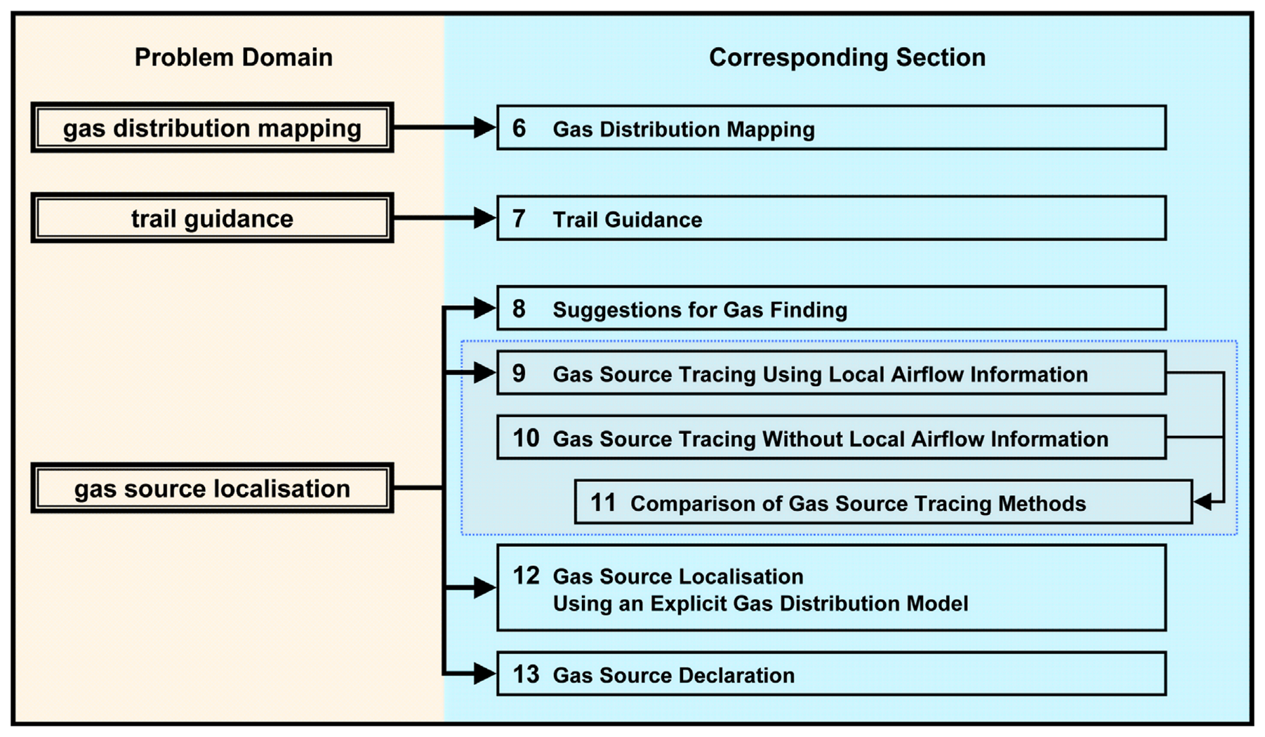
Figure 5.
Mapped gas distribution in a wind tunnel adapted from Pyk et al. [60]. The gas source was placed at (x,y) = (0 m, 1.5 m) and the wind direction was the positive x-axis direction. Left: a map obtained from sequential measurements with a single sensor array (static response map). At each location where the sensor was placed (shown in the image as white dots), the response was averaged over 2 minutes and the time-averaged values were interpolated using bi-cubic filtering. Middle: a map created from the response of a gas sensor array carried by a mobile robot at a speed of approx. 10 cm/s (dynamic response map). Here, the sensor response was interpolated between the trace of the robot (indicated by a dashed line) using triangle-based cubic interpolation. Right: dynamic response map obtained by averaging over three runs. The response strength is given in arbitrary units as indicated in the legends.
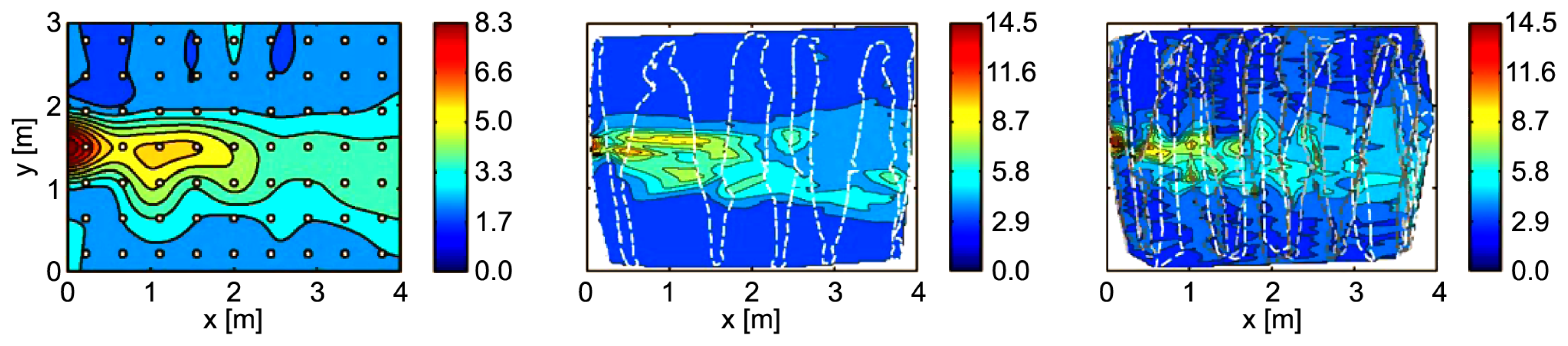
Figure 6.
Visualisation of the number of odour hits (i.e. how often the sensor response exceeded a predefined threshold) recorded by six robots while performing a random walk behaviour for one hour. The left figure shows a visualisation of the two-dimensional histogram which is obtained by accumulating the odour hits received by all the robots. The spatial distribution of odour hits received by the individual robots can be seen in the six sub-images on the right side. The source location corresponds to the upper right corner of these subimages. Adapted from Hayes et al. [16]

Figure 7.
Examples of kernel-extrapolated gas distribution gridmaps created from concentration data collected with a gas-sensitive mobile robot up to the time specified. The cell size is 2.5 × 2.5 cm2.
Figure 7.
Examples of kernel-extrapolated gas distribution gridmaps created from concentration data collected with a gas-sensitive mobile robot up to the time specified. The cell size is 2.5 × 2.5 cm2.

Figure 8.
Air curtain technique. (a) Illustration of the functional principle, adapted from Russell et al. [68]. Air is drawn from the floor through the sensor inlet and blown in the opposite direction around the sensor inlet. Thus, an outward airflow is created that is able to deflect gas carried towards the sensor by external air currents. (b) Image of the mobile robot “Nose-Bot” equipped with the improved gas sensor (photograph by courtesy of R. Andrew Russell).
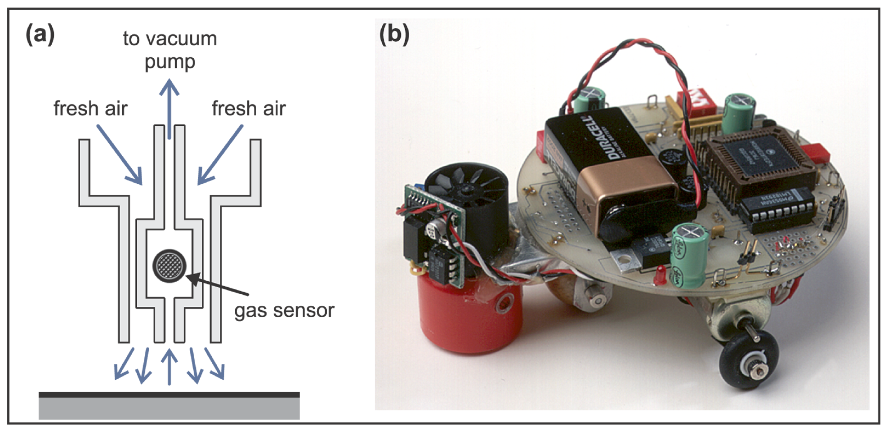
Figure 9.
Trail following strategies with a pair of sensors. (a) Chemo-tropotaxis to keep a pair of sensors over the trail. (b) Chemo-tropotaxis to keep the trail between the pair of sensors. (c) Timeout mechanism to increase robustness against measurement errors or intermittent trails. The idealised trail is indicated by a bright grey vertical stripe. A star around a sensor indicates that this sensor detects the trail.

Figure 10.
Trail guidance strategies with a single gas sensor. (a) Repellent chemical marker. The example shows cleaning robots that use an odourous trail to indicate the area that has already been cleaned. (b) Trail following with a single gas sensor [8].
Figure 10.
Trail guidance strategies with a single gas sensor. (a) Repellent chemical marker. The example shows cleaning robots that use an odourous trail to indicate the area that has already been cleaned. (b) Trail following with a single gas sensor [8].
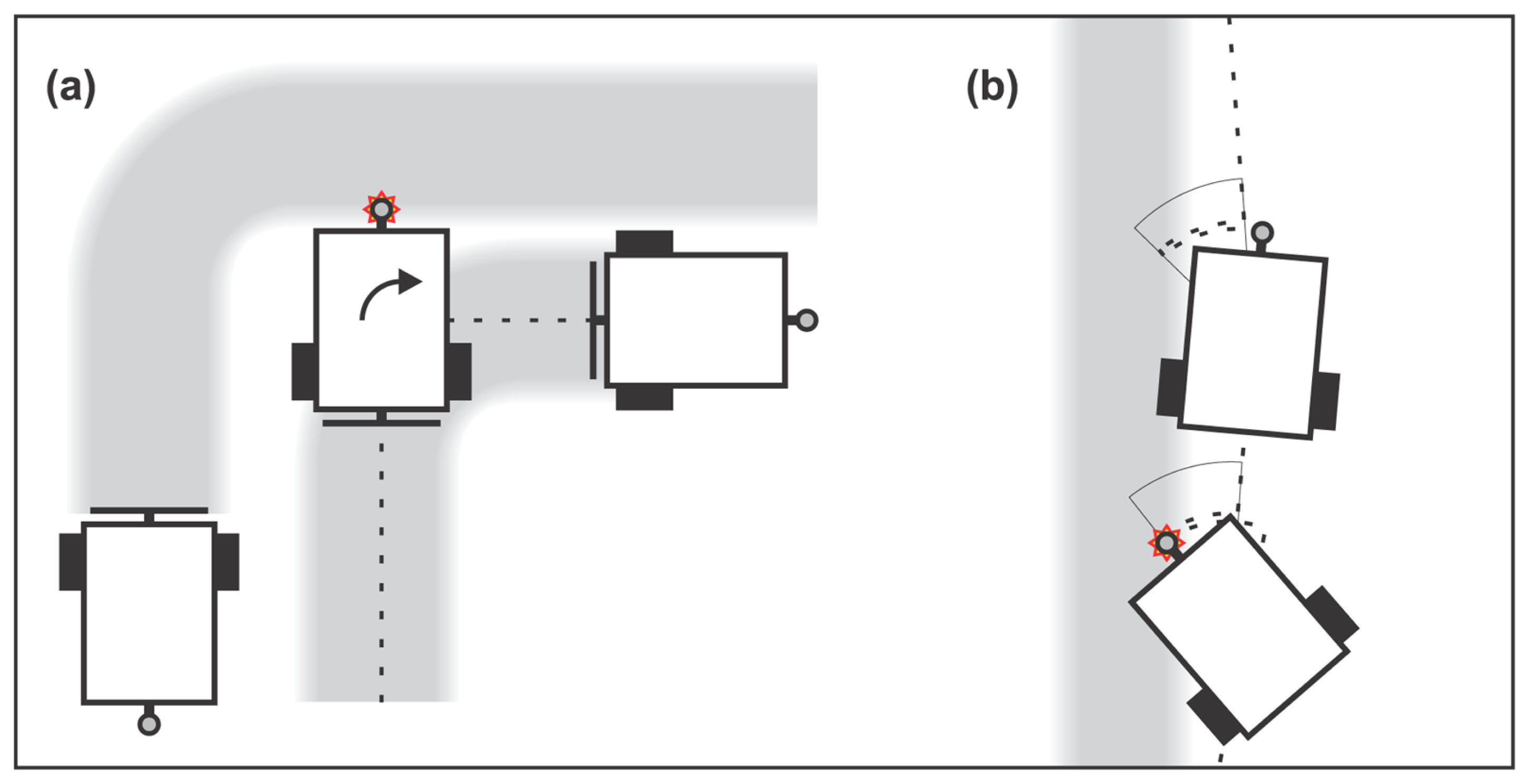
Figure 11.
Sensor probe used in the experiments of Ishida et al. [76], which consists of four thermistor anemometric sensors and four metal oxide gas sensors. (a) Sketch of the probe, adapted from [76]. (b) Mobile robot carrying the sensor probe (photograph by courtesy of Hiroshi Ishida).
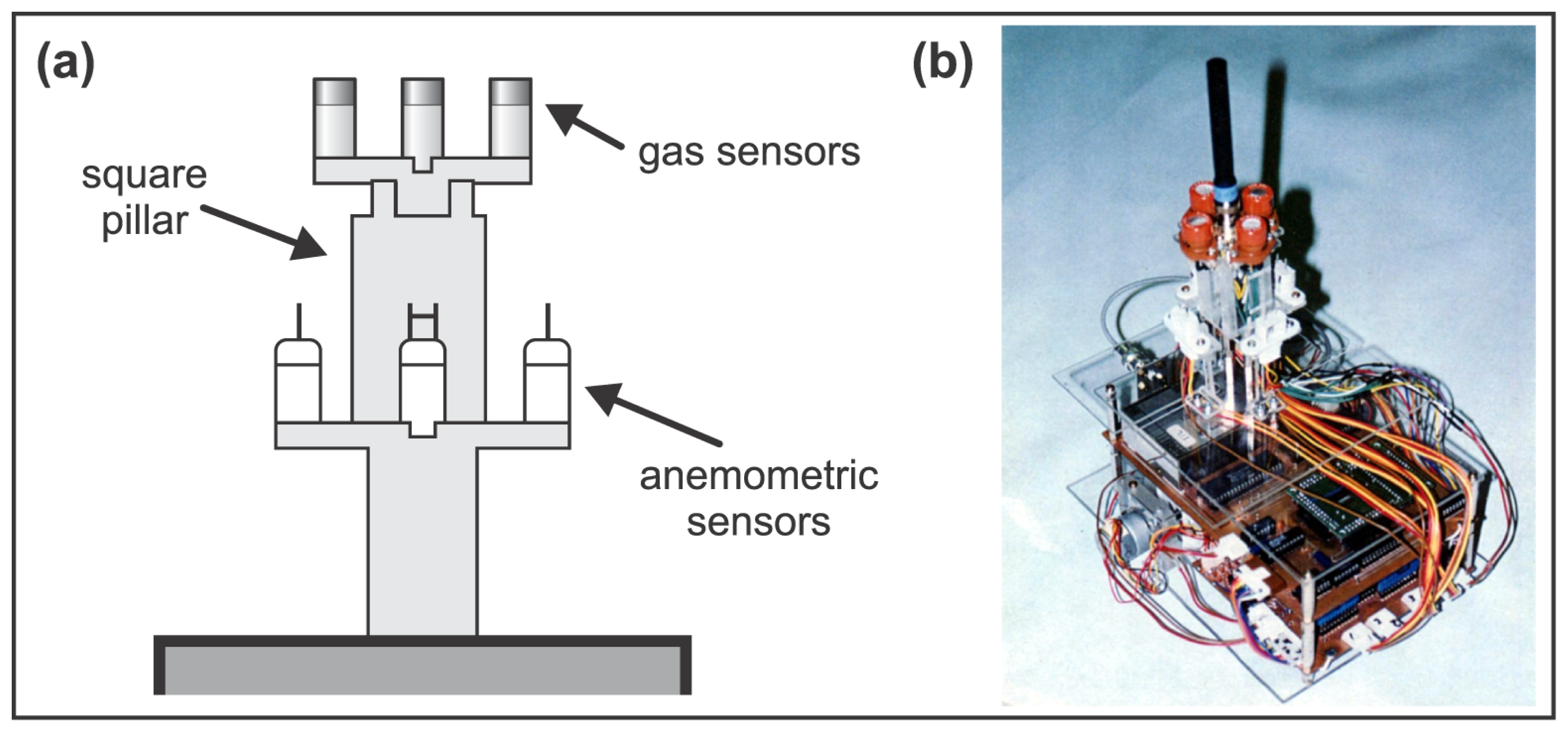
Figure 12.
(a) Step-by-step progress method suggested by Ishida et al. [76]. The wind direction was determined with an accuracy of 90 ° in this experiment. For clarity of the illustration, a larger step length (in proportion to the size of the robot) than used in the actual experiments is assumed in the sketch. (b) Zigzag approach method [76]. The wind direction was determined with an accuracy of 45 ° in this experiment. Possible trajectories are indicated on top of an idealised gas plume. A star around a sensor indicates that this sensor detects the target gas.

Figure 13.
(a) Plume-centred upwind search by Russell et al. [77]. (b) Bombyx mori algorithm as implemented by Russell and co-workers in [75]. Possible trajectories are plotted on top of the idealised gas distribution assumed by the particular strategy.
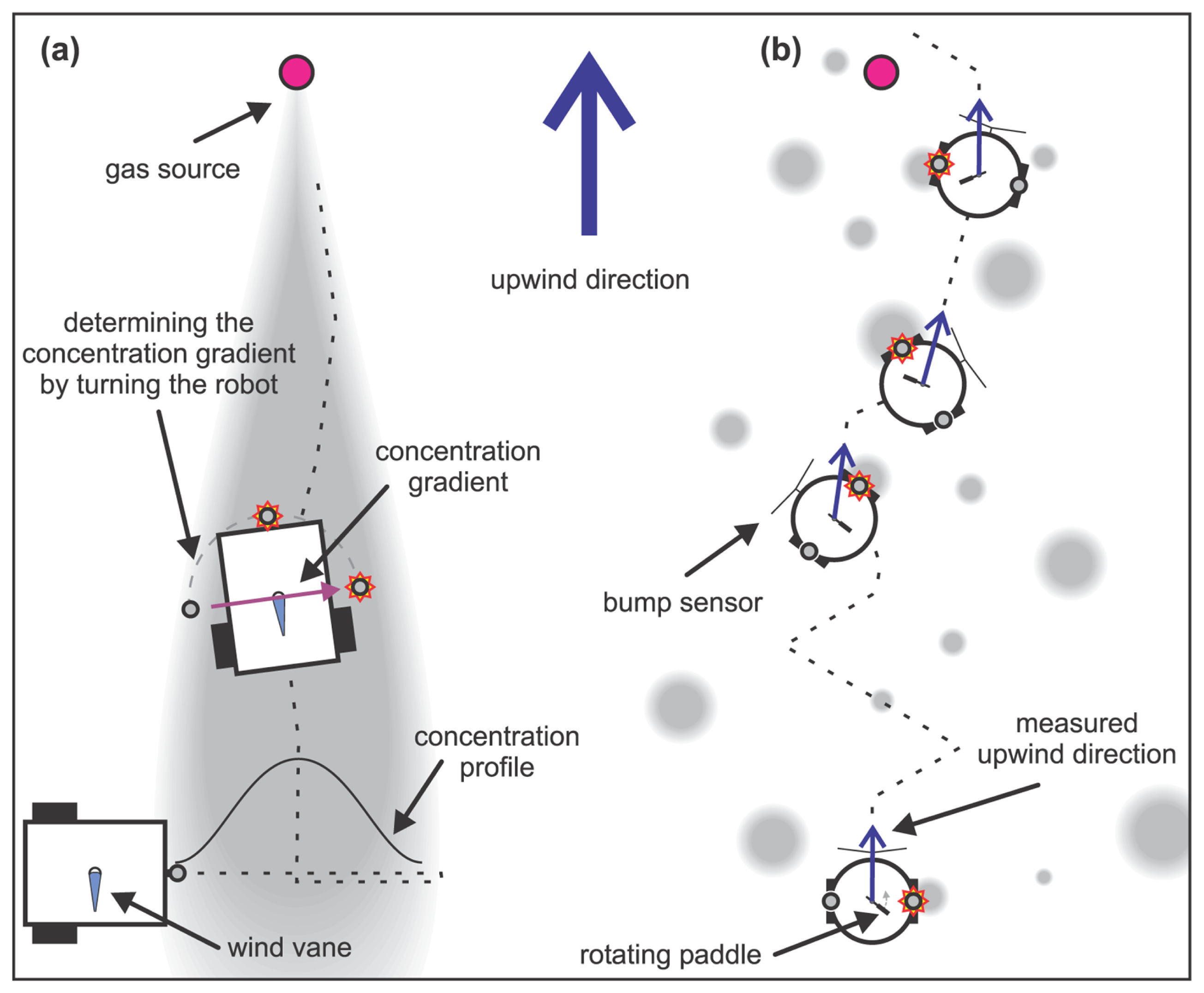
Figure 14.
(a) Dungbeetle G. stercorarius algorithm, Russell et al. [75]. (b) Spiral surge algorithm, Hayes et al. [16].
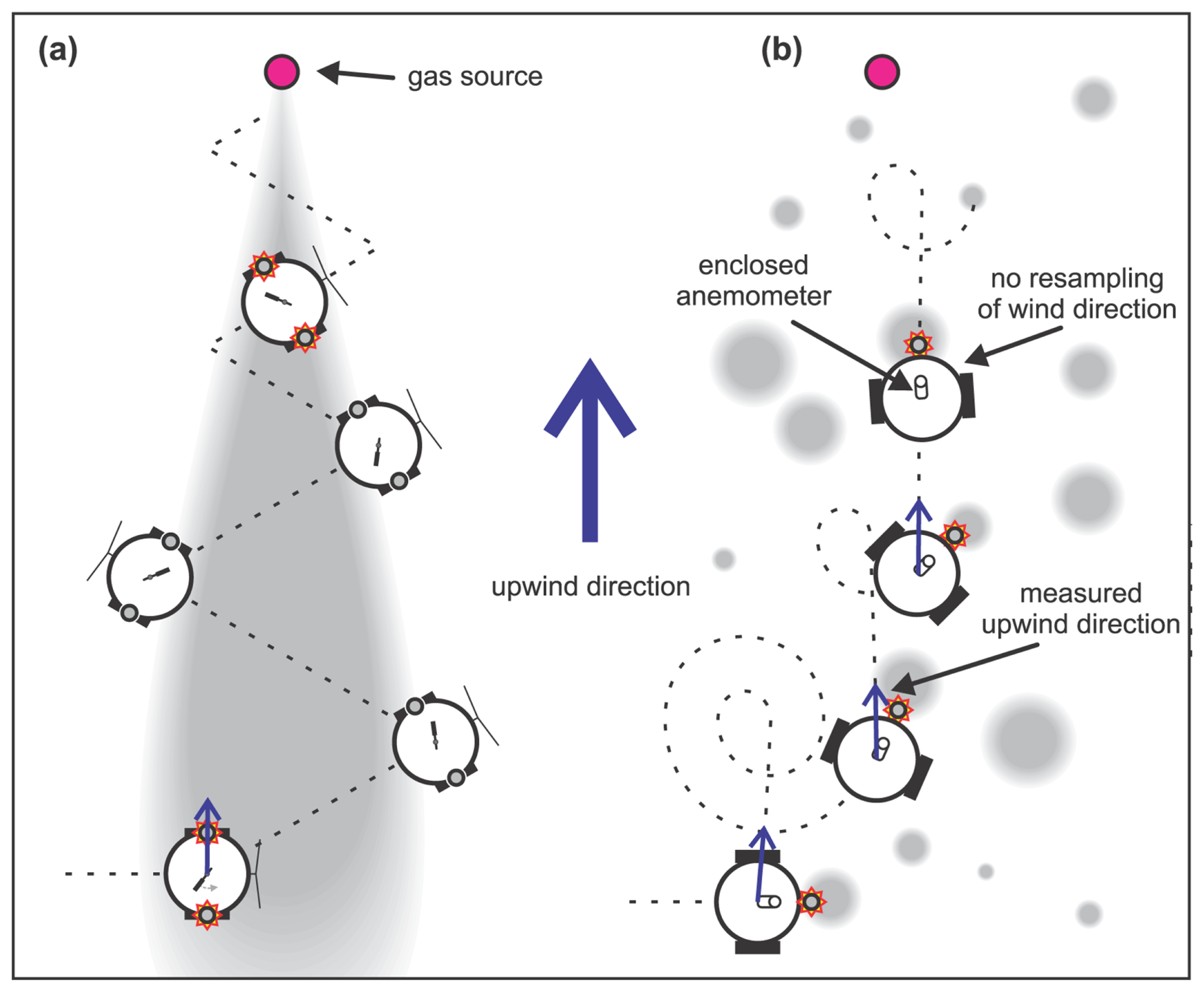
Figure 15.
Multiphase tracing algorithm (Ishida et al. [83]).
Figure 15.
Multiphase tracing algorithm (Ishida et al. [83]).
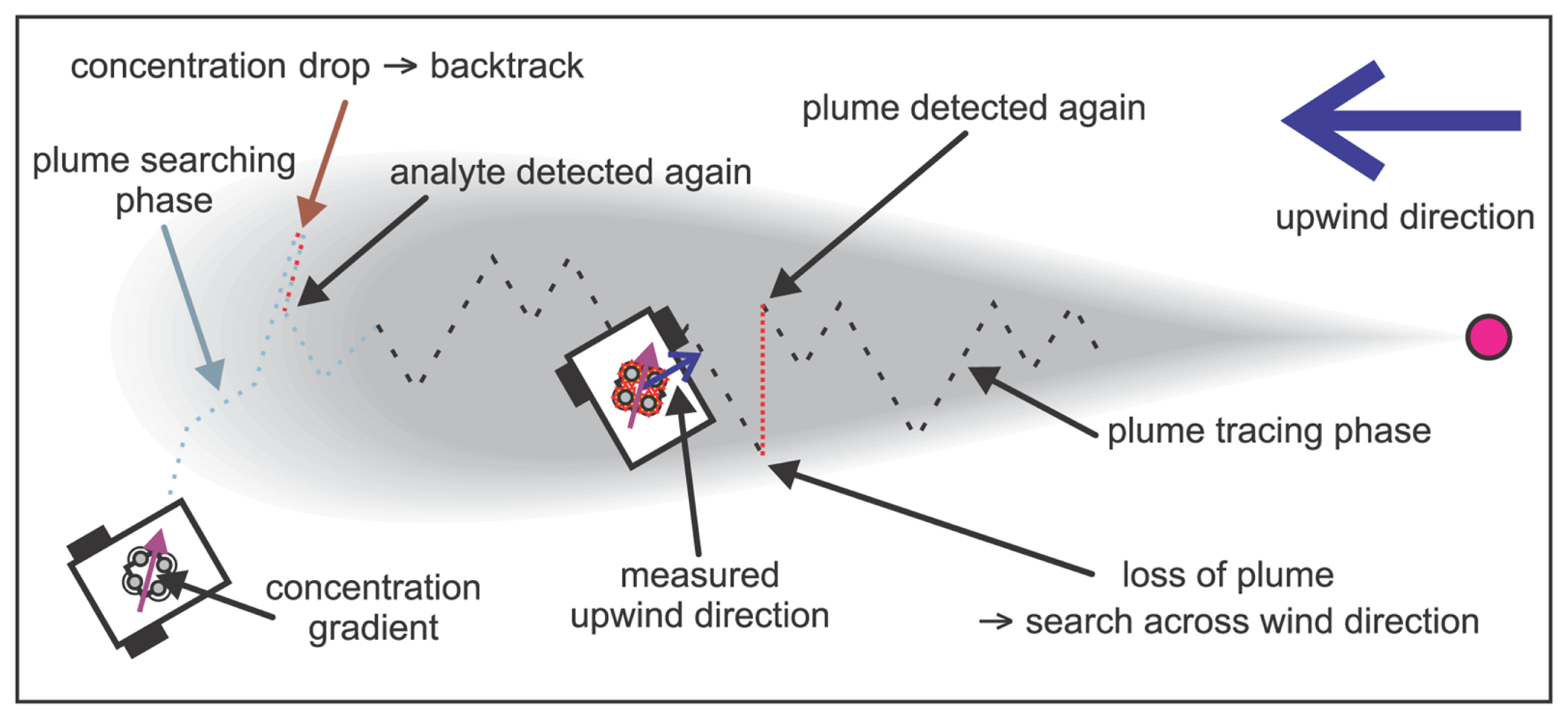
Figure 16.
(a) Sketch that shows the functional principle of the two-dimensional odour compass (top view), adapted from [5]. (b) Three-dimensional odour compass (by courtesy of Hiroshi Ishida).
Figure 16.
(a) Sketch that shows the functional principle of the two-dimensional odour compass (top view), adapted from [5]. (b) Three-dimensional odour compass (by courtesy of Hiroshi Ishida).
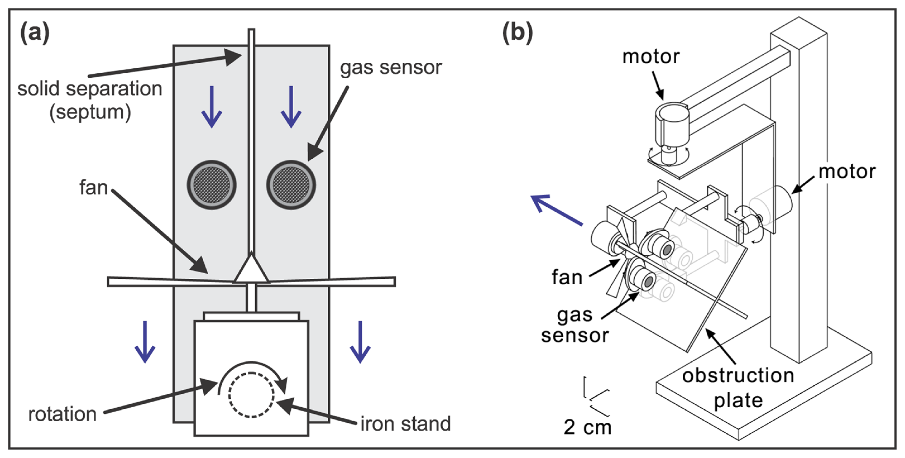
Figure 17.
(a) Schematic diagram of the blimp-based robot used for three-dimensional gas source tracing experiments by Ishida et al. [86]. (b) Sketch of the corresponding experimental setup.
Figure 17.
(a) Schematic diagram of the blimp-based robot used for three-dimensional gas source tracing experiments by Ishida et al. [86]. (b) Sketch of the corresponding experimental setup.
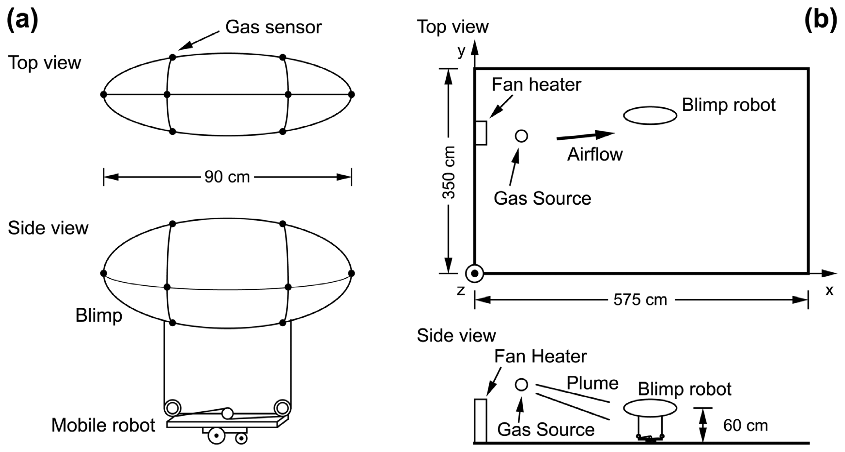
Figure 18.
(a) Sketch of the gas source. (b) Koala robot with the Örebro Mark III mobile nose in front of the dripping gas source. (c) Schematic view of the direct (inhibitory) sensor-motor coupling (Braitenberg vehicles).
Figure 18.
(a) Sketch of the gas source. (b) Koala robot with the Örebro Mark III mobile nose in front of the dripping gas source. (c) Schematic view of the direct (inhibitory) sensor-motor coupling (Braitenberg vehicles).
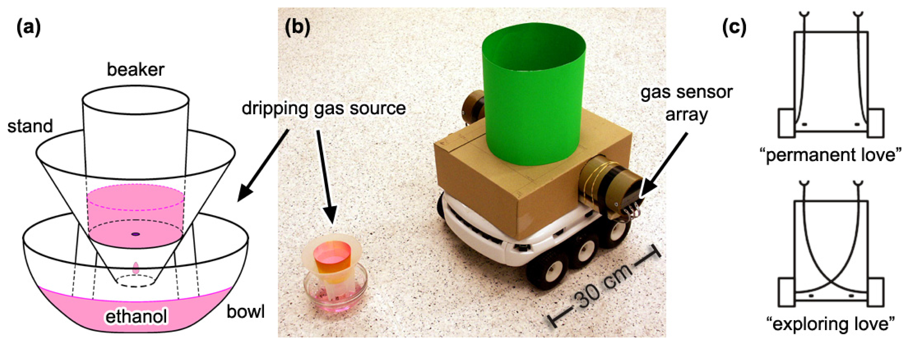
Figure 19.
Example paths of the Braitenberg vehicle plotted on top of the gas concentration gridmap calculated from all the trials of the corresponding sequence with the mapping method by Lilienthal and Duckett described in Section 6. The path of the robot's centre is indicated by small circles, while the position of the front corners is plotted using small dots. The starting position and the initial heading of the corresponding trial are marked by an arrow. Also shown are the boundaries of the testbed area by two broken lines that mark the area where the robot is exposed to an increasing repellent force. The clearance area of the gas source, which was located in the middle of the testbed area in all trials shown, is indicated by two circles (the outer one is derived by obstacle growing assuming a circular robot).
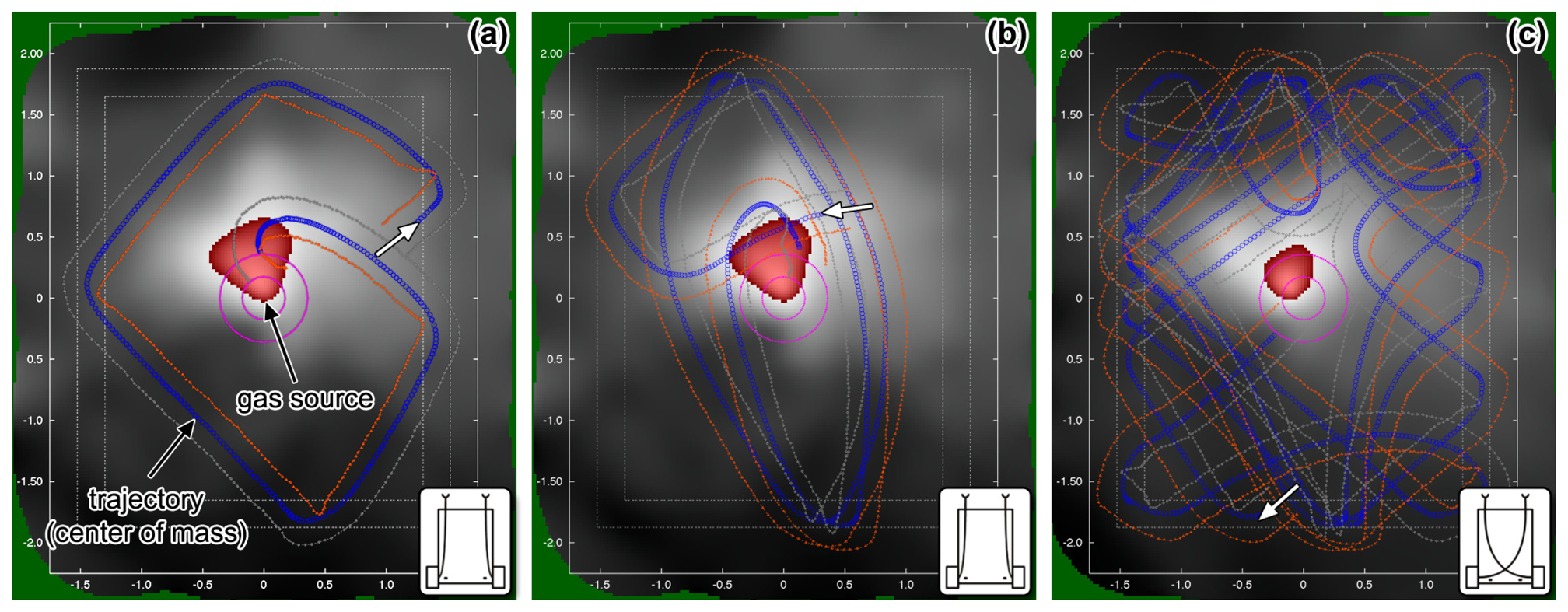
Figure 20.
Gas source tracing strategy based on the behaviour of Bombyx mori males, and adapted for the condition that no information about air currents is available. The figure shows the fixed motion pattern, which is executed in response to an increased gas concentration.
Figure 20.
Gas source tracing strategy based on the behaviour of Bombyx mori males, and adapted for the condition that no information about air currents is available. The figure shows the fixed motion pattern, which is executed in response to an increased gas concentration.
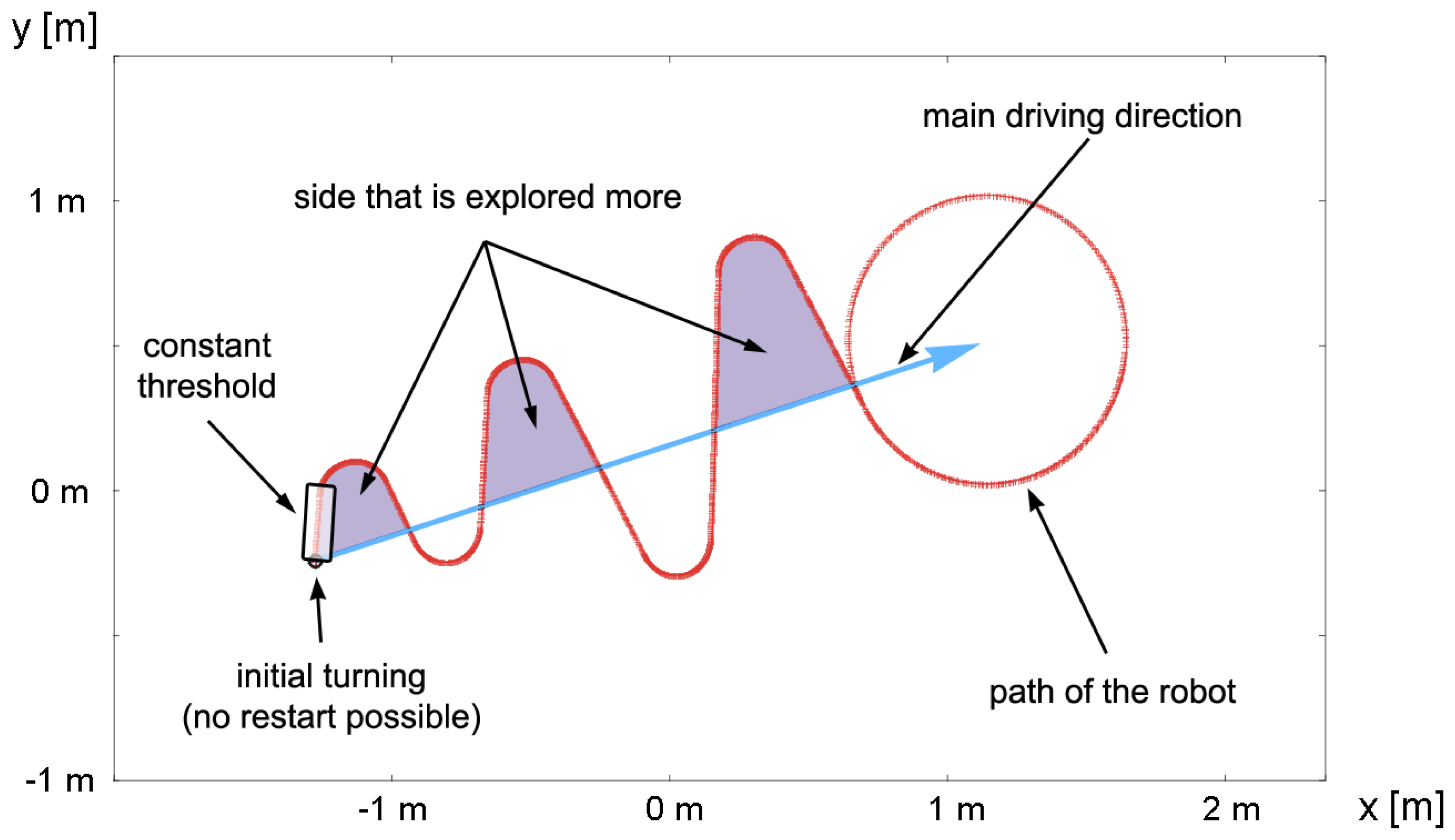
Figure 21.
The Örebro Mark I (a), and the Örebro Mark II mobile nose (b).
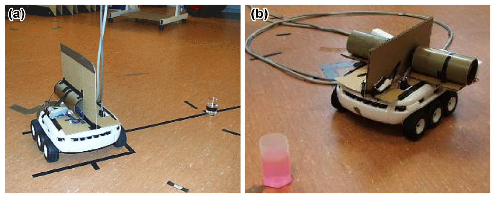
Figure 22.
(a) The gas-sensitive mobile robot Arthur in front of the source used in the gas source declaration experiments by Lilienthal et al. This distance was considered as being directly in front of the source. (b) Comparison of the classification performance obtained with an optimised threshold classifier and a support vector machine. The achieved hit rate is plotted against the average distance of negative examples from the gas source.
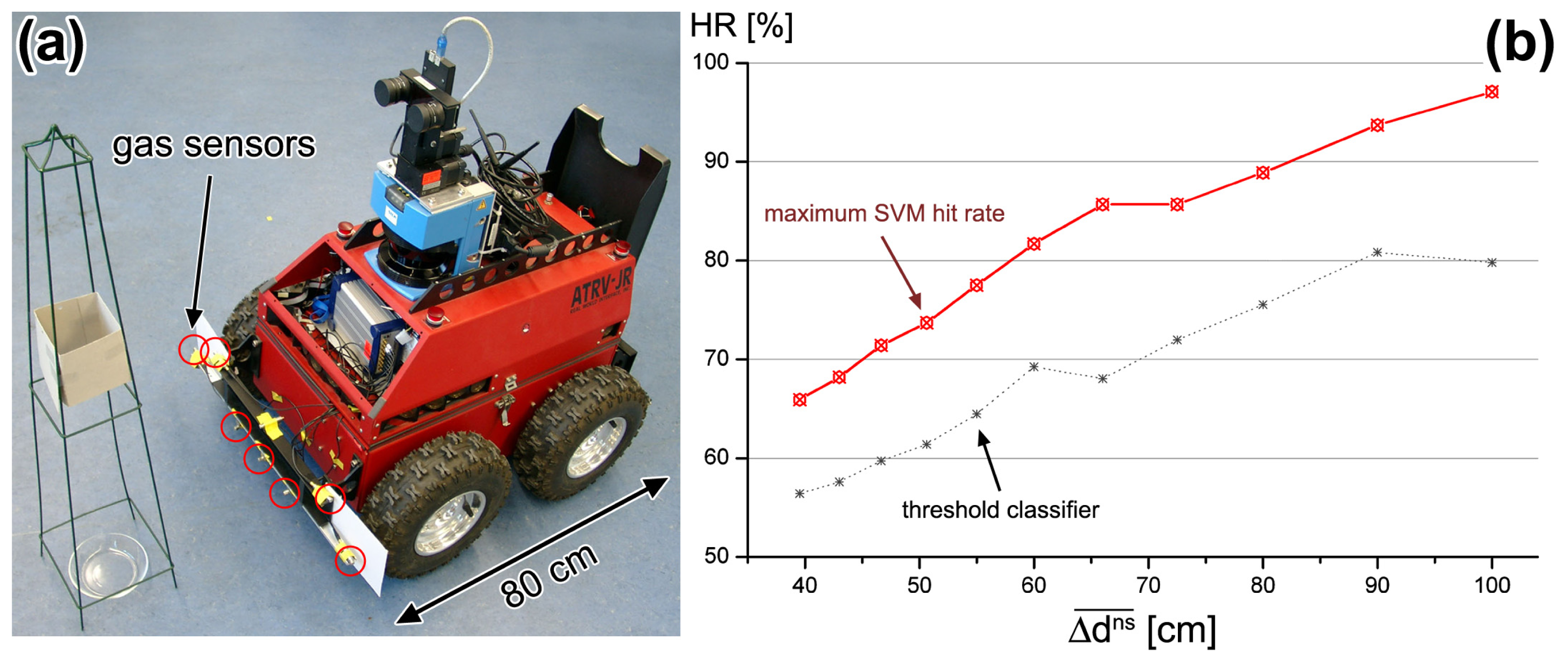
Figure 23.
Comparison of (a) average trial response, (b) standard deviation during a trial, and (c) standard deviation divided by the average trial response, all measured against the average distance to the gas source dAv. Each figure shows the average of the respective indicator over the trials with a particular distance from the gas source. The respective standard deviation is indicated by error bars.
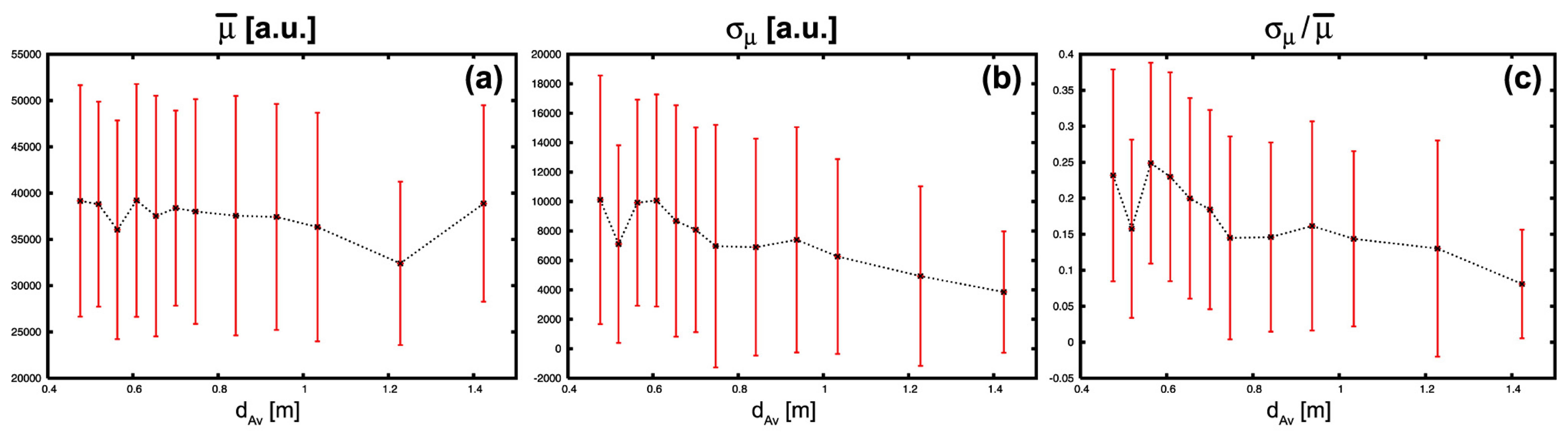

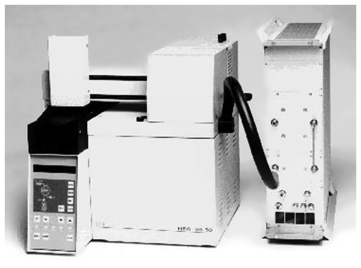
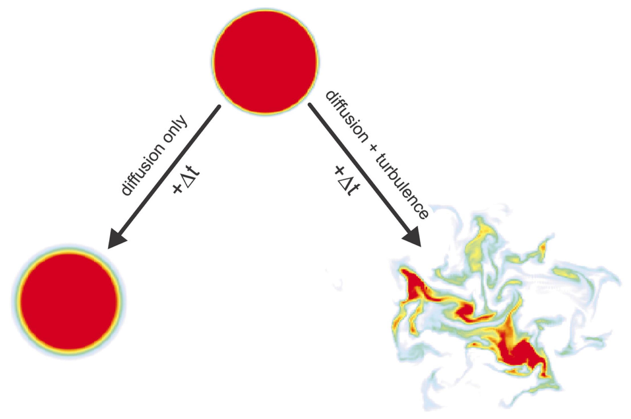
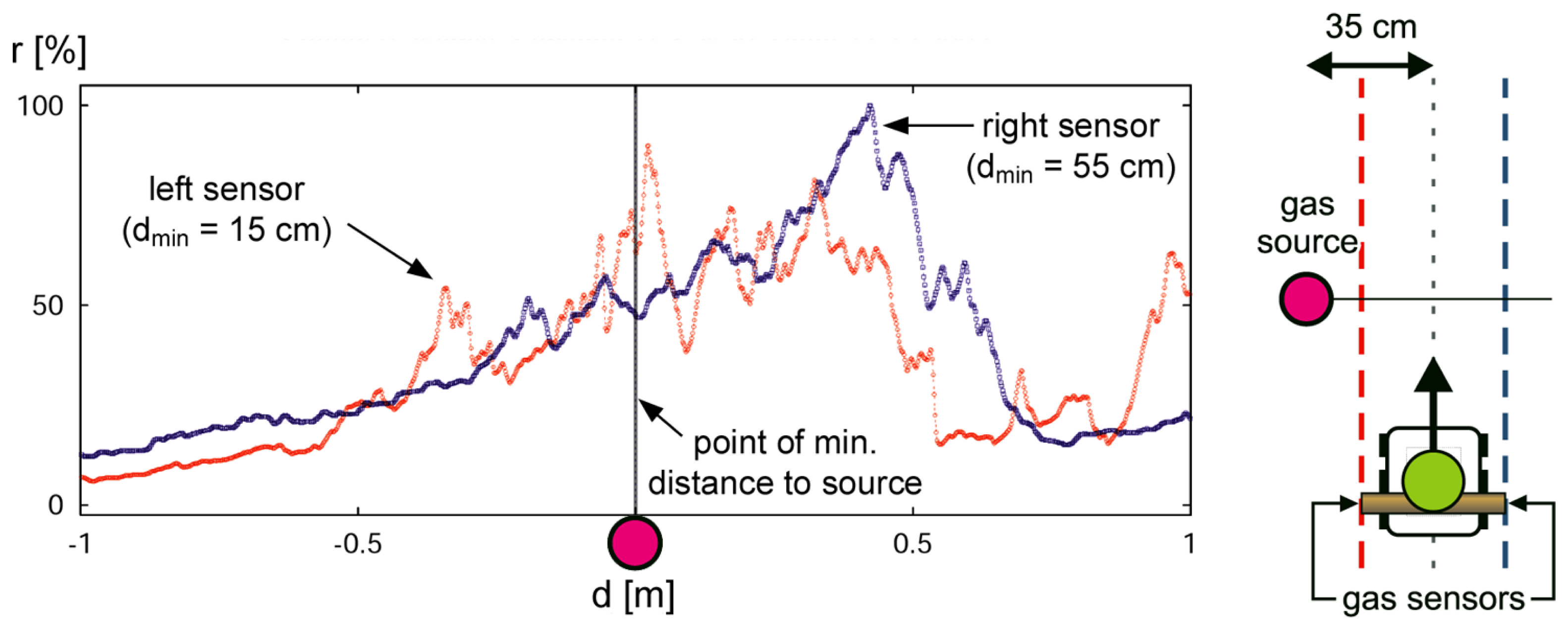
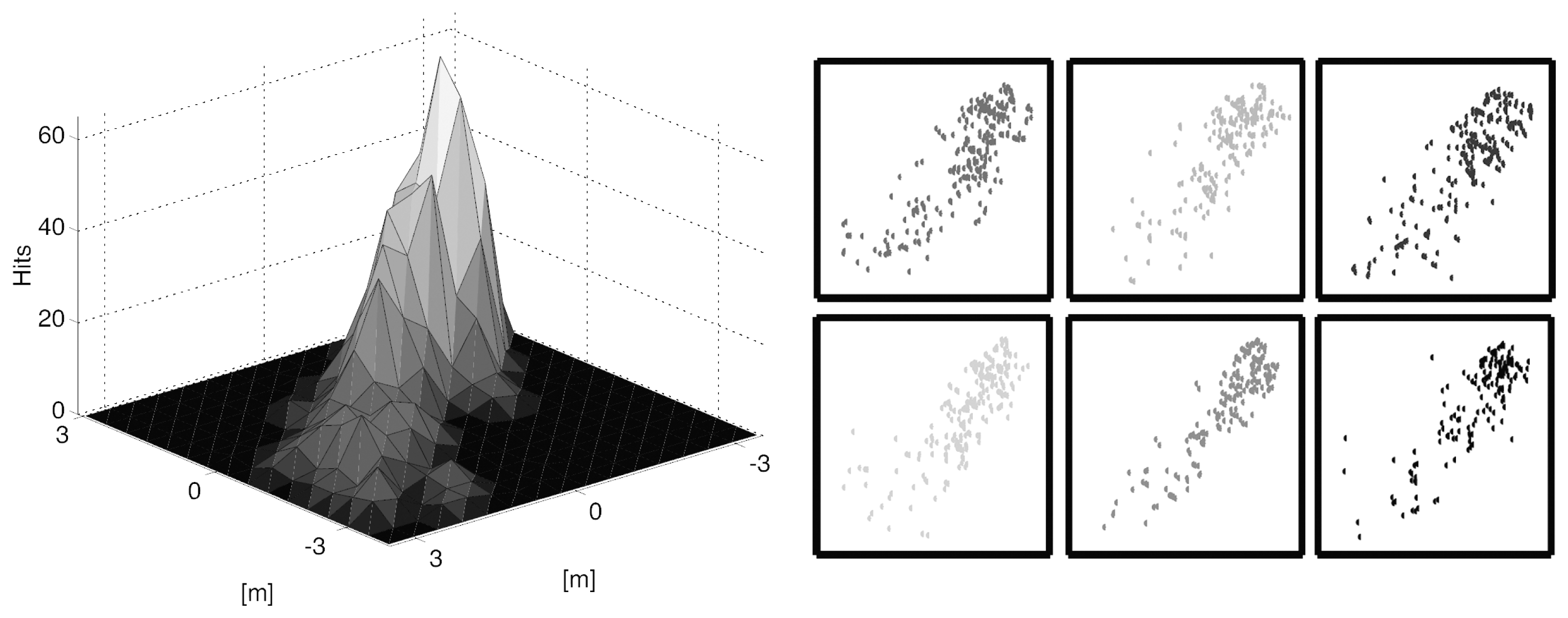
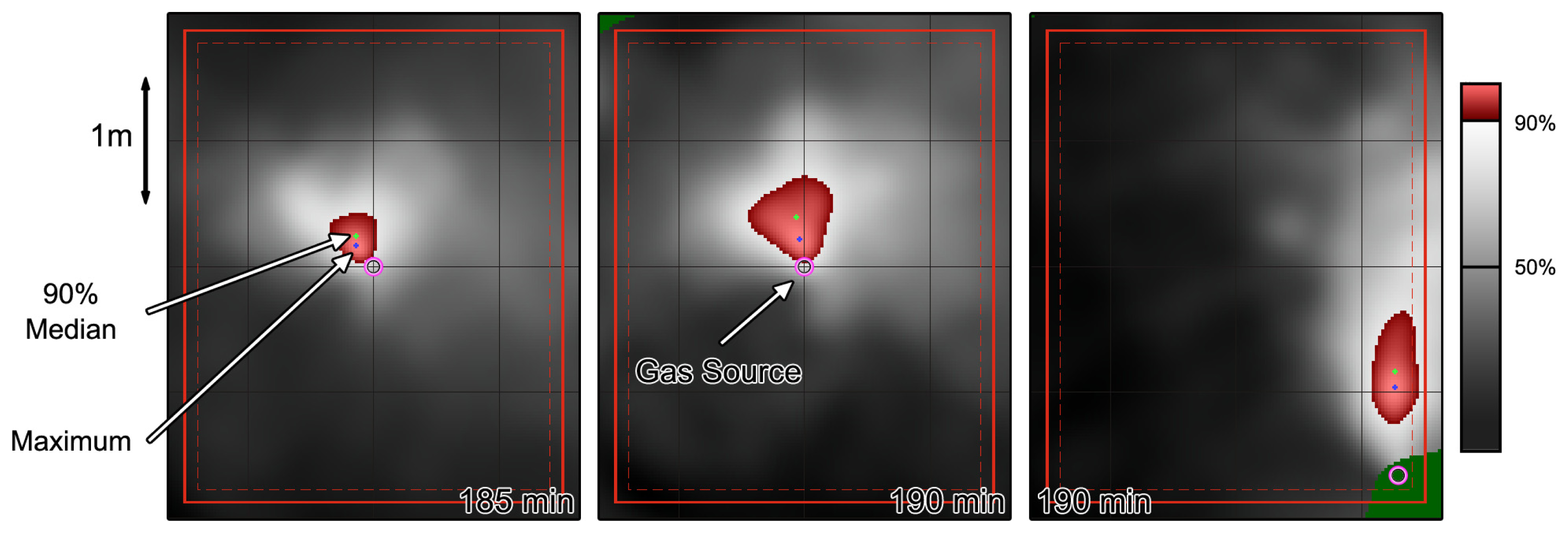
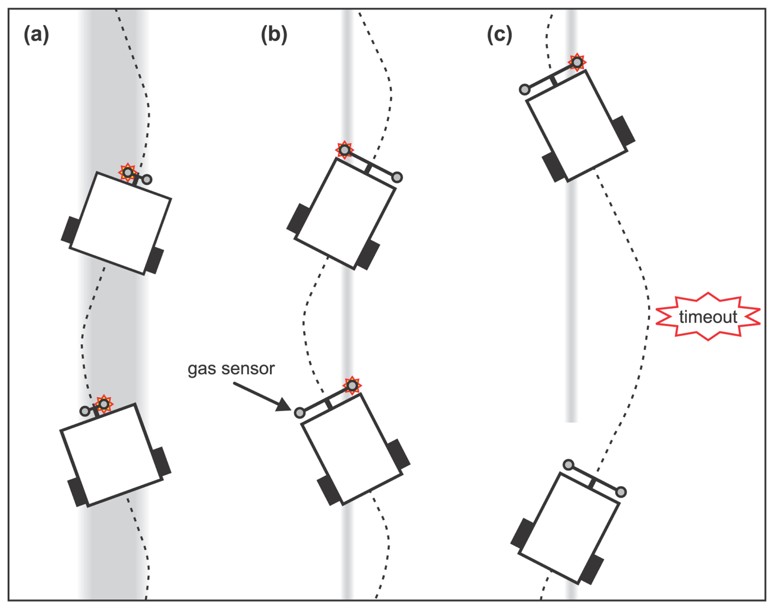
Table 1.
Gas source tracing strategies that were experimentally tested on a mobile robot and require information about the local wind vector.
| Strategy | Min. Requirements/Implementation/Experiment |
|---|---|
| zigzag approach Section 9.2, [76] Fig. 12 (b) | 1 gas sensor, directional wind sensor upwind plume crossing with turns at the edge of the plume + backtracking uniform air flow (≈ 12 or 20 cm/s), tracing distance ≈ 80 cm |
| dung beetle algorithm Section 9.5, [75] Fig. 14 (a) | 1 gas sensor, directional wind sensor upwind plume crossing with turns at the edge of the plume uniform air flow (≈ 1.5 m/s), tracing distance ≈ 2 m |
| plume-centred upwind search Section 9.3, [77] Fig. 13 (a) | 1 gas sensor, directional wind sensor upwind movement with corrections of the heading after each step according to the concentration gradient across the upwind direction uniform air flow (≈ 30 cm/s), tracing distance ≈ 1 m |
| step-by-step progress Section 9.1, [76] Fig. 12 (a) | 2 gas sensors, directional wind sensor simultaneous concentration gradient following across the wind and up-wind movement + waiting period (if concentration is low) uniform air flow (≈ 12 or 20 cm/s), tracing distance ≈ 80 cm |
| spiral surge algorithm Section 9.8, [16] Fig. 14 (b) | 1 gas sensor, directional wind sensor surge in upwind direction with a subsequent local search (outward spiral) triggered by high concentrations uniform air flow (≈ 1 m/s), tracing distance ≈ 6 m |
| Bombyx mori algorithm Section 9.4, [75] Fig. 13 (b) | 2 gas sensors, directional wind sensor local search biased by the wind direction and the concentration gradient, triggered by high concentrations uniform air flow (≈ 1.5 m/s), tracing distance ≈ 2m |
| multiphase tracing algorithm Section 9.9, [83] Fig. 15 | 2 gas sensors, directional wind sensor gradient-following if concentration is low, upwind movement and gradient-following across the wind otherwise + backtracking non-uniform air flow (≈ 10 - 30 cm/s), tracing distance ≈ 1.5 m |
Table 2.
Gas source tracing strategies that were experimentally tested on a mobile robot and do not require information about the airflow.
| Strategy | Min. Requirements/Implementation/Experiment |
|---|---|
| E. coli algorithm Section 9.6, [75] | 1 gas sensor straight “runs” and direction randomising “tumbles”, longer runs if concentration increases, higher tumbling frequency otherwise uniform air flow (≈ 1.5 m/s), no successful tracing trials |
| iterative chemo-tropotaxis Section 9.7, [75] | 2 gas sensors turn towards the higher concentration by a small angle, move forward, repeat uniform air flow (≈ 1.5 m/s), tracing distance ≈ 2 m |
| gas-sensitive Braitenberg vehicle Section 10.2, [99] | 2 gas sensors uncrossed inhibitory sensor-motor connection (exploration and hill-climbing) unventilated environment, tracing distance 1 m - 4 m |
| 3D chemotaxis Section 9.11.1, [86] | 10 gas sensors move towards the sensor with the highest response (averaging time: 20 s) ventilated environment, air flow ≈ 0.5 m/s, tracing distance 2.2 m |
| modified Bombyx mori algorithm Section 10.3, [13] Fig. 20 | 2 gas sensors local search biased by the initially sensed concentration gradient, triggered by high concentrations unventilated environment, initial distance to the source 2.75 m - 8.4 m (no indication that the source was found) |
| neural network controller Section 10.4, [95] | 2 gas sensors rotational speed of the robot controlled by the output of a feedforward neural network (trained with 7 different directions) weak airconditioning, tracing distance 80 cm |
© 2006 by MDPI ( http://www.mdpi.org). Reproduction is permitted for noncommercial purposes.
Share and Cite
MDPI and ACS Style
Lilienthal, A.J.; Loutfi, A.; Duckett, T. Airborne Chemical Sensing with Mobile Robots. Sensors 2006, 6, 1616-1678. https://doi.org/10.3390/s6111616
AMA Style
Lilienthal AJ, Loutfi A, Duckett T. Airborne Chemical Sensing with Mobile Robots. Sensors. 2006; 6(11):1616-1678. https://doi.org/10.3390/s6111616
Chicago/Turabian StyleLilienthal, Achim J., Amy Loutfi, and Tom Duckett. 2006. "Airborne Chemical Sensing with Mobile Robots" Sensors 6, no. 11: 1616-1678. https://doi.org/10.3390/s6111616