Envisat Ocean Altimetry Performance Assessment and Cross-calibration

1
Collecte Localisation Satellite (CLS), 8-10 rue Hermès, 31526 Ramonville St-Agne, France
2
Centre National d’Etudes Spatiales (CNES), DCT/PO/AL BPI 2002, 18, Av. Edouard Belin 31401 Toulouse Cedex 9, France
3
European Space Agency, EO Ground Segment Department, ESA/ESRIN EOP-GOQ, Via Galileo Galilei CP64, Frascati, Italy
*
Author to whom correspondence should be addressed.
Sensors 2006, 6(3), 100-130; https://doi.org/10.3390/s6030100
Submission received: 16 September 2005
/
Accepted: 21 February 2006
/
Published: 3 March 2006
(This article belongs to the Special Issue Satellite Altimetry: New Sensors and New Application)
Abstract
:Nearly three years of Envisat altimetric observations over ocean are available in Geophysical Data Record (GDR) products. The quality assessment of these data is routinely performed at the CLS Space Oceanography Division in the frame of the CNES Segment Sol Altimétrie et Orbitographie (SSALTO) and ESA French Processing and Archiving Center (F-PAC) activities. This paper presents the main results in terms of Envisat data quality: verification of data availability and validity, monitoring of the most relevant altimeter (ocean1 retracking) and radiometer parameters, assessment of the Envisat altimeter system performances. This includes a cross-calibration analysis of Envisat data with Jason-1, ERS-2 and T/P. Envisat data show good general quality. A good orbit quality and a low level of noise allow Envisat to reach the high level of accuracy of other precise missions such as T/P and Jason-1. Some issues raised in this paper, as the gravity induced orbit errors, will be solved in the next version of GDR products. Some others, as the Envisat Mean Sea Level in the first year, still need further investigation.
1. Introduction
Since its launch in March 2002, the European earth observation satellite Envisat has been providing measurements of the atmosphere, ocean, land, and ice. This advanced polar-orbiting satellite ensures the continuity of the altimetric observations started with the ERS-1 satellite in 1991, but with higher precision. Among many instruments, the satellite carries a new generation of dual frequency radar altimeter (RA-2) which allows correction of ionosphere effects, a microwave radiometer (MWR) and a laser reflector and a Doris receiver which highly improve the accuracy of the orbit determination.
Extensive work has been produced during the Envisat verification phase by the Cross-Calibration and Validation Team (CCVT) to check the quality of the Envisat altimetric measurements. Since September 2003, the GDR products have been routinely produced and disseminated. Envisat altimeter system quality is continuously checked by the Quality Working Group (QWG) members. First results from GDR data have been presented during the 2004 Symposium meeting in Salzburg (e.g. Dorandeu et al. 2004 [1]).
This paper is basically concerned with long-term monitoring of the Envisat altimeter system over ocean. Indeed continuous quality control of the altimetric data is essential. These data are used by many applications, from scientific research to operational oceanography, that require a high level of accuracy. Improving altimetric data performances should also help developing new applications.
Data from GDR cycles 10 through 38 spanning nearly three years have been used for this analysis. All relevant altimeter parameters deduced from Ocean 1 retracking, radiometer parameters and geophysical corrections are evaluated and tested. This work is routinely performed at CLS, as part of the SSALTO and funded by ESA through F-PAC activities. In this frame, besides continuous analyses in terms of altimeter data quality, Envisat GDR Quality Assessment Reports (e.g. Faugere et al. 2003 [2]) are routinely produced in conjunction with data dissemination.
The work performed in terms of data quality assessment also includes cross-calibration with Jason-1, ERS-2 and T/P. This kind of comparisons between coincident altimeter missions provides a large number of estimations and consequently efficient long-term monitoring of instrument measurements. This enables the detection of instrument drifts and inter-mission biases essential to obtain a consistent multi-satellite data set. Envisat Sea Level Anomalies (SLA) are also compared to an independent dataset, a tide gauge network.
After a preliminary section describing the data used, the paper is split into four main sections: first, data coverage and measurement validity issues are presented. Second, monitoring of the main altimeter and radiometer parameters is performed, describing the major impact in terms of data accuracy. Then, performances are assessed and discussed with respect to the major sources of errors. Finally, Envisat Sea Surface height (SSH) bias and MSL issues are analyzed.
2. Data used and processing
Envisat Geophysical Data Records (GDRs) from cycle 10 to cycle 38 have been used to derive the results presented in this paper. This corresponds to a nearly three-year time period spanning from September 30th 2002 to July 11th 2005. The routine production started on September 2003 with cycle 15. In parallel, a backward reprocessing of cycle 14 to 9 has been implemented. With only 7 days of available data, cycle 9 has not been used in this work. Note that cycles 1 to 8, corresponding to the in-flight calibration period, have not been disseminated by ESA. All these data have been processed in the same ground processing version except cycles 15 to 18. On November 26th 2003, the Instrument Processor Facility (IPF) version changed from 4.55 to 4.56. Consequently, from cycle 19 onwards and for the reprocessed cycles 10 to 14, the Automatic Gain Control (AGC) evaluation and the Intermediate Frequency (IF) mask correction (with slight impact on the data) have been modified.
To perform this quality assessment work, conventional validation tools are used including editing procedures, crossover analysis, collinear differences, and a large number of statistical monitoring and visualization tools. All these tools are integrated and maintained as part of the CNES SSALTO (Segment Sol Altimétrie et Orbitographie) ground segment and F-PAC (French Processing and Archiving Centre) tools operated at CLS premises. Each cycle is carefully routinely analyzed before data release to end users. The main data quality features are reported in a cyclic quality assessment report (Faugere et al., 2003 [2]).
As for all other existing altimeters, the Envisat GDR data are ingested in the Calval 1-Hz altimeter database maintained by the CLS Spatial Oceanography Division. This allows us to cross-calibrate and cross-compare Envisat data to other missions. In this study data from Jason-1 (from GDRs cycles 27 to 129), ERS-2 (from OPRs cycles 78 to 105), and TOPEX tandem data (from T/P MGDR_B cycles 370 to 472) are used. Jason-1 is the most suitable for Envisat cross calibration as it is available throughout the Envisat mission and has been extensively calibrated to T/P (Dorandeu et al., 2004b [3]). Comparisons between Jason-1 and Envisat altimeter and radiometer parameters have been carried out using 10-day dual crossovers for SSH comparison and 3-hour dual crossovers for altimeter and radiometer comparisons. The geographical distribution of the dual crossovers with short time lags strongly changes from one Envisat cycle to another. Indeed, contrary to Envisat which is sun-synchronous, Jason-1 observes the same place at the same local time every 12 cycles (120-day). Following the method detailed in Stum et al. [4], estimates of the differences are computed using a 120 day running window to keep a constant geographical coverage. ERS-2, flying on same ground track as Envisat only 30 minutes apart, has had a coverage limited to the North Atlantic since the failure of the on-board register in June 2003 (EOHelp message of 4 July 2003). To improve the significance of the Envisat/ERS-2 comparison, long term monitoring of altimeter parameters difference is performed on this restricted area all over the Envisat period using a repeat-track method. T/P is used for global cross comparisons of the mean sea level trend as this mission provides a precise long term reference.
Most of this work has been carried out using parameters available in the GDR products. However, a few updates have been necessary to complete the analyses. First, as Jason-1 doesn't fly at the same altitude as Envisat, and ERS-2 has a mono-frequency altimeter on-board, it is not possible to use these satellites to assess the Envisat ionosphere path delay. Thus the JPL GPS-based global Ionospheric Maps (GIM) containing the vertical ionospheric total electron content are used here. Then, another set of orbits have been tested. They have been generated by the DEOS institute at Delft Institute of technology using the Grace Gravity Model EIGEN-GRACE01S instead of GRIM5 (Doornbos et al., 2005 [5]) currently used for operational orbit computation. A correction to the range is also applied based on the Ultra-Stable Oscillator (USO) clock period variation correction. The USO, which performs the computation of the RA-2 window time delay, is affected by a drift due to the ageing of the device. The method to correct this is described in Celani [6]. The correction is regularly updated in the IPF ground processing via an auxiliary data file. However, due to an anomaly in the ADF format, the correction is not taken into account (Martini, 2003 [7]) in the products. This anomaly will be corrected in the next IPF version. For the time being, ESA supplies auxiliary files to allow users to correct their own database [8]. Finally, pressure values used for computing the inverse barometer and the dry troposphere corrections have been derived from the ECMWF rectangular grids. Errors due to the bathymetry, up to several centimeters near the coasts, significantly impact the accuracy of the so-called gaussian grids used as input of the Envisat (and Jason-1) ground processing (e.g. Dorandeu et al., 2004 [3]).
3. Data coverage and edited measurements
This section mainly intends to analyze the ability of the Envisat altimeter system to correctly sample ocean surfaces. This obviously includes the tracking capabilities, but also the frequency of unavailable data and the ratio of valid measurements likely to be used by applications after the editing process.
3.1 Missing measurements
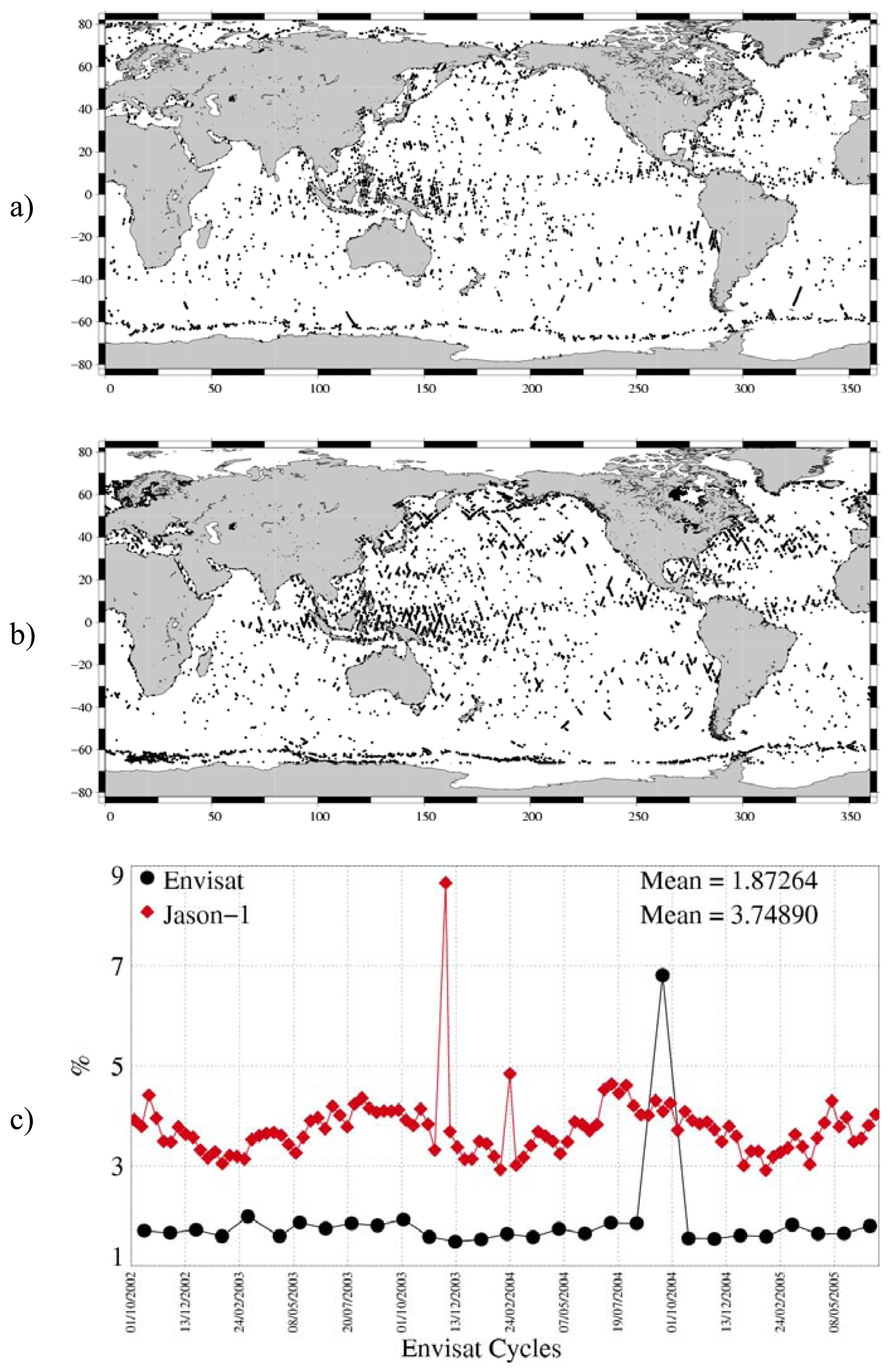
From a theoretical ground track, a dedicated collocation tool allows determination of missing measurements relative to what is nominally expected. The cycle by cycle percentage of missing measurements over ocean has been plotted in Figure 1a. The measurement unavailability is more than 8% in average. Seven cycles have more than 10% of unavailability, notably from cycle 13 to cycle 17. Passes 1 to 452 of cycle 15 have not been delivered because of a wrong setting of RA-2. This explains the high ratio of missing measurements for this cycle. Several long RA-2 events occurred during cycles 13, 14, 16, 17, 22 and 34 which resulted in a significant number of missing passes. Apart from instrumental and platform events, up to 3% of measurements can be missing because of data generation problems at ground segment level. Notice however that the situation has been largely improved with a mean data availability of more than 95% from the beginning of 2004 (cycle 23 onwards).
Figure 1b shows an example of missing measurements for cycle 25. Within this cycle, 9 passes are completely missing along with segments missing from several other passes. The measurements which are missing over the Himalayan region are due first to the IF Calibration Mode. Moreover, daily instrument switch-offs (Heater 2 mode) are performed over this region to prevent the S-Band anomaly. Apart from that, the data retention rate is very good on every surface observed. This might be due to the tracker used by Envisat Ra-2, the Model Free Tracker (MFT).
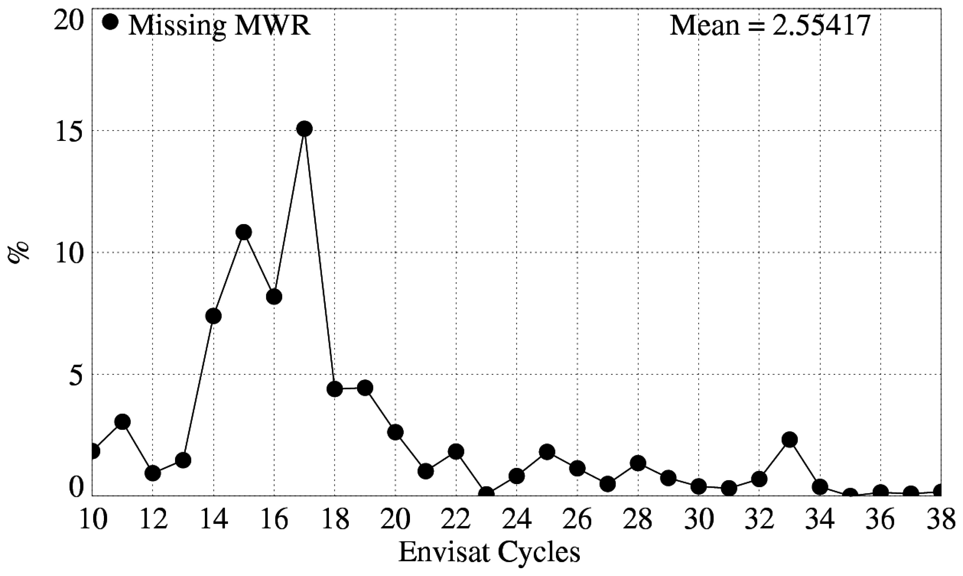
The Envisat MWR provides nearly 100% availability of data since the beginning of the mission (Dedieu et al., 2005 [9]). However, MWR corrections can be missing in the GDRs due to data generation problems at ground segment level. The ratio of missing MWR corrections has been plotted in Figure 2. The mean value is around 2.6% but the radiometer unavailability is not constant. It is greater than 4% for cycles 14 to 19 but lower than 2% from cycle 21 onwards. From cycle 34 onwards the availability of the MWR correction is almost 100%, which is encouraging.
3.2 Edited measurements
Data editing is necessary to remove altimeter measurements having lower accuracy. The first step of the editing procedure consists in removing data impacted by the S-Band anomaly or corrupted by sea ice. During the Commissioning Phase, it has been discovered that the RA-2 data are affected by the so-called S-Band anomaly. The anomaly results in the accumulation of the S-Band echo waveforms (Laxon and Roca, 2002 [10]). It happens randomly after an acquisition sequence and is only stopped by switching the RA-2 in a stand-by mode. When this anomaly occurs, the S-Band waveforms are not meaningful. Consequently, all the S-Band parameters and the dual-frequency ionosphere correction are not reliable. Notably, the S-band sigma0 is unrealistically high during these events. Thus applying a threshold of 5 dB on the (Ku-S) sigma0 differences is very efficient for detecting the impacted data over ocean. The ratio of flagged measurements over ocean is plotted in Figure 3. Between 0 and 8% of the data are impacted. From cycle 31 onwards, some modifications have been performed by ESA to decrease the duration of these events: instrument switch-offs (Heater 2 mode) are performed twice a day over the Himalayan region. This prevents the S-Band anomaly from lasting more than half a day when it occurs. Thanks to this procedure the ratio of impacted data decreased from 4.2% (cycles 11 to 30) to 2.2% (cycles 31 to 38). A method has been developed to flag the impacted data over all surfaces (Martini et al., 2005 [11]). It will be available in the next GDR version. The reconstruction of normal echoes from accumulated waveforms is also currently under study (Martini et al., 2005 [11]).
Since Envisat operates between ±82° of latitude, sea ice is an important issue for oceanic applications. No ice flag is currently available in the Envisat products, therefore alternate sea ice detection techniques are employed in order to retain only open ocean data. A study performed during the validation phase showed that the combination of altimetric and radiometric criteria was particularly efficient to flag most of the data over ice. The method is described in detail in (Faugere et al, 2003 [12]). We employ the peakiness parameter (Lillibridge et al, 2005 [13]) in conjunction with the MWR- ECMWF wet troposphere difference which appears to be a good means to complement the peakiness parameter in all ice conditions.
The second step of the editing procedure consists in using thresholds on several parameters., The minimum and maximum thresholds used in the routine quality assessment are given in (Faugere et al., 2004 [14]). The thresholds are expected to remain constant throughout the ENVISAT mission, so that monitoring the number of edited measurements allows a survey of data quality. This method is used for T/P and Jason-1 [3] and is applied on Envisat to ensure the consistency among the different missions. However, note that useful quality flags, such as the rain flag, are available in the product.
The percentage of edited measurements over ocean for the main altimeter and radiometer parameters has been plotted in Figure 4. These ratios are very stable and surprisingly low over the period if compared to other altimeters. The RMS of elementary measurements has the strongest ratio among the altimeter parameters, more than 1%. A slight seasonal signal is visible on the curve, mostly due to sea state seasonal variations. The number of elementary measurements has a surprisingly low ratio, except for cycles 14 and 20 when wrong configuration files were uploaded onboard after a RA-2 event. The square of the off-nadir angle derived from waveforms leads to very stable editing ratio. Variations of this parameter can reveal actual platform mispointing, if any, but can also reveal waveform contamination by rain or by sea-ice. It is indeed computed from the slope of trailing edge when fitting a typical ocean model to the waveforms. No seasonal signal is visible which may prove that the sea-ice detection method is efficient. The dual-frequency ratio shows a slight increasing trend between cycles 15 and 28 which cannot be considered as significant, given the scatter of the curve. The Ku-band SWH, sigma0 and MWR ratios are very stable and low, less than 0.2% with no seasonal variations.
It has been necessary to apply additional editing criteria on SSH-MSS differences in order to remove remaining spurious data. The first criterion consists in removing measurements with SSH-MSS greater than 2m. The ratio is plotted in Figure 4e. The high value on cycle 30 is due to abnormal behavior of the RA-2 sensor during nearly two days. Just after a RA-2 recovery, the range value jumped by several meters for a still unexplained reason. The second criterion was necessary to detect measurements impacted by maneuvers. Maneuvers are necessary to compensate the effect of gravitational forces but can have a strong impact on the orbit quality. Two types of maneuvers are operated to maintain the satellite ground track within the +/-1km deadband around the reference ground track: in-plane maneuvers, every 30-50 days, which only impact the altitude of the satellite and out-of-plane maneuvers, three times a year, to control the inclination of the satellite (Rudolph et al., 2005 [15]). The out-of-plane maneuvers are the most problematic for the orbit computation. The second criterion consists in testing the mean and standard deviation of the SSH-MSS over each entire pass. If one of the two values, computed on a selected dataset, is abnormally high, then the entire pass is edited. The criteria for selecting the area and the thresholds are detailed in (Faugere et al., 2004 [14]). On cycles 11, 12, 21 and 26, several full passes have been edited because of bad orbit quality related to out-of-plane manoeuvre or lack of Doris data (cycle 11).
The Envisat editing ratios are significantly lower than those observed on other altimeters like Jason or T/P. In Figure 5a and b the Envisat map of edited measurements is compared to the equivalent map on Jason-1. The edited measurement density of Envisat is much lower than the Jason-1 one, especially in wet areas, where altimeter measurements are likely to be corrupted by rain. The cycle by cycle ratio of edited measurements for both satellites is plotted in Figure 5c. It shows that, except on particular cycles, Envisat ratios are lower than Jason-1 ones by 1 to 2%. As previously mentioned this might be explained by different tracker processing. Notice that more data appear over Antartica on the Jason-1 map. It highlights that the Jason-1 sea ice flag proposed in GDRs, used in the first step, is not efficient enough to remove all the data corrupted by sea ice. The method used for Envisat is more efficient.
4. Long term monitoring of altimeter and radiometer parameters
All GDR fields are systematically checked and carefully monitored as part of the Envisat routine calibration and validation tasks. However, only the main Ku-band parameters are presented here, as they are the most significant in terms of data quality and instrumental stability. Furthermore, all statistics are computed on valid ocean datasets after the editing procedure.
4.1 Number and standard deviation of 20Hz elementary Ku-band measurements
As part of the ground segment processing, a regression is performed to derive the 1 Hz range from 20 Hz data. Through an iterative regression process, elementary ranges too far from the regression line are discarded until convergence is reached. The mean number and RMS of Ku 20Hz elementary data used to compute the 1Hz average are plotted in Figure 6. These two parameters are nearly constant, which provides an indication of the RA-2 altimeter stability. The mean number of Ku 20Hz values over one cycle is about 19.97. This value is very high compared to other altimeters. It is almost the same in wet areas or near the coast. The two drops on the Ku-band on cycles 14 and 20 are due to wrong setting of the RA-2 just after recovery. A slight seasonal signal is visible on the mean RMS of Ku 20Hz. Higher values correspond to higher waves occurring during the austral winter. The mean value is about 9.0 cm. This value represents a rough estimation of the 20 Hz altimeter noise (Zanifé et al. 2003 [16], Vincent et al. 2003a [17]). Assuming that the 20Hz measurements have uncorrelated noise, it corresponds to a noise of about 2 cm at 1Hz, which is consistent with the expected noise values.
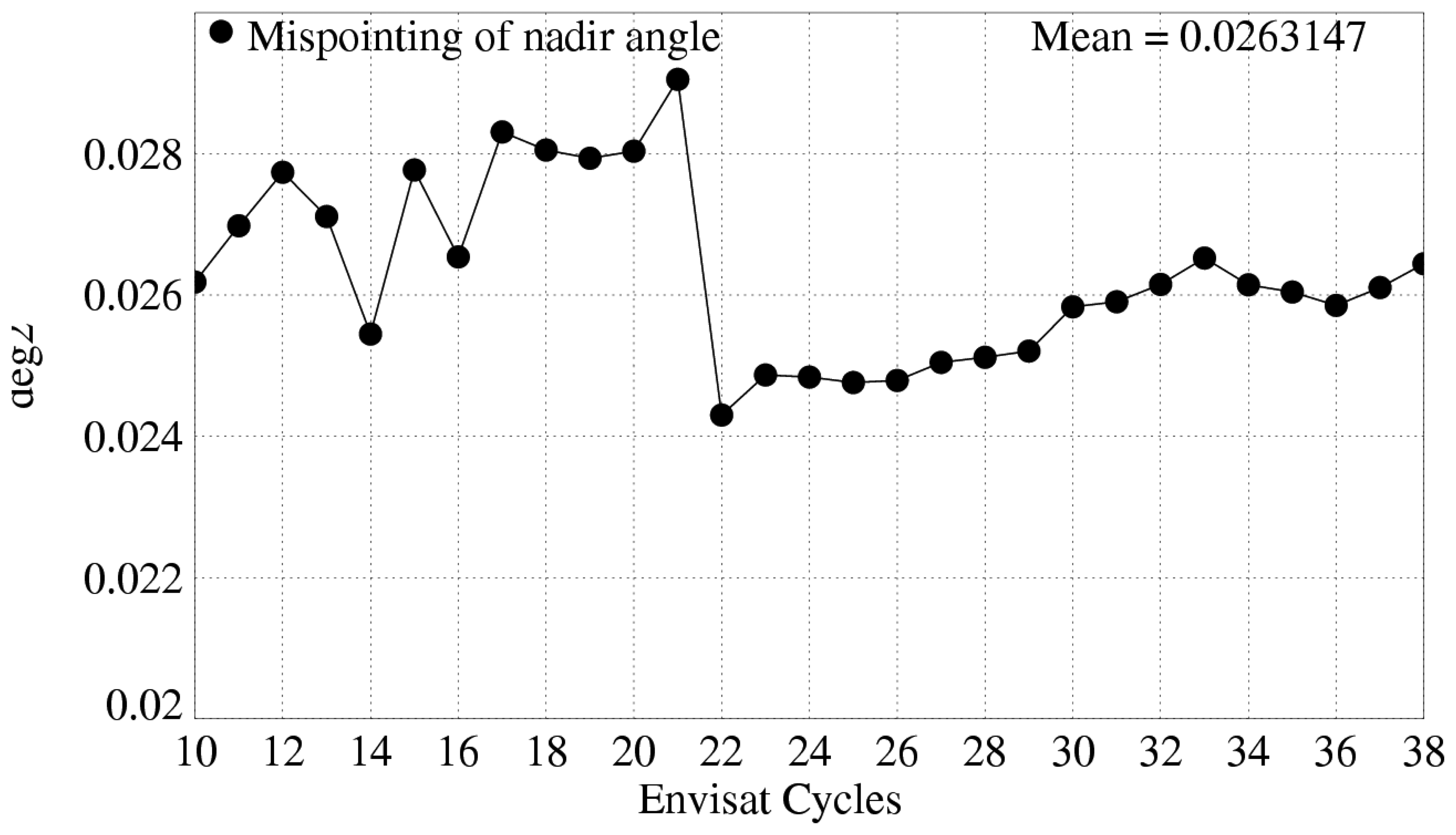
4.2 Off-nadir angle from waveforms
The off-nadir angle is estimated from the waveform shape during the altimeter processing. The square of the off-nadir angle is plotted in
Figure 7. The mean value is about 0.026 deg2. This mean value is not significant in terms of actual platform mispointing. This is due to the way the slope of the waveform trailing edge is computed and will be corrected in the next GDR version. The 0.005 deg2 jump between cycles 21 and 22 is due to the upgrade of the IF mask filter auxiliary data file. The slight rising trend observed on the curve might be due to the onboard filter which is not current (last update was November 2003).
4.3 Significant Wave Height
The cycle by cycle mean and standard deviation of Ku and S-band SWH are plotted in Figure 8a and b. The curve reflects sea state variations. The mean value of Ku SWH is 2.66 m. The S-band mean SWH is very close, less than 10 cm apart. The cycle by cycle mean of Envisat-Jason-1 differences and ERS-2-Envisat differences are plotted in Figure 8c and d. These differences are quite stable. Envisat SWH is respectively 15 cm and 22 cm higher than Jason-1 and ERS-2 SWH.
4.4 Backscatter coefficient
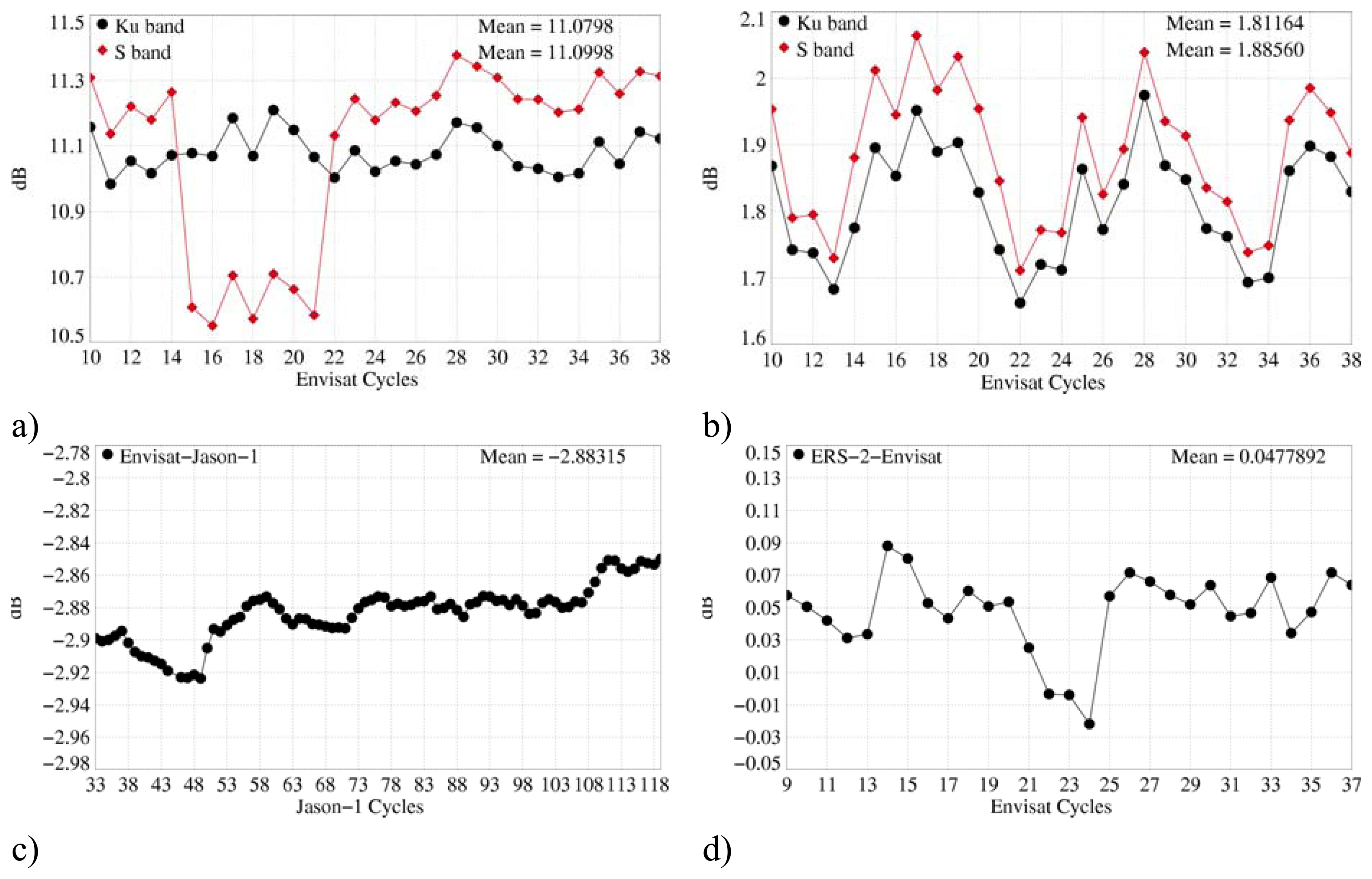
The cycle by cycle mean and standard deviation Ku and S-band Sigma0 are plotted in Figure 9a and b. Note that a -3.5 dB bias has been applied (Roca et al., 2003 [18]) on the Ku-band Sigma0 in order to be compliant with the wind speed model (Witter and Chelton, 1991 [19]). The mean values in Ku band are stable, around 11.1 dB. Two 0.66 dB jumps are visible on the S-Band on cycles 14 and 22. They are due to a correction of the AGC evaluation. This modification has been included in IPF version 4.56, used from cycle 22 onwards for the current processing and for all the reprocessed cycles. The cycle by cycle mean of Envisat-Jason-1 differences and ERS-2-Envisat differences are plotted in Figure 1c and d. The mean difference between Envisat and Jason-1 Ku-band Sigma0 is -2.9 dB. This mean difference has increased by 0.07dB between cycles 48 and 118 which corresponds to 0.04 dB/year. This trend, though not really significant, has to be monitored in the next cycles. The mean ERS-2-Envisat Ku-band Sigma0 difference is 0.05 dB. However, this mean value accounts for the calibration correction applied in the ground processing to enter the wind speed algorithm (Witter and Chelton, 1991 [19]).
4.5 Dual-frequency ionosphere correction
As performed on TOPEX (Le Traon et al. 1994 [20]) and Jason-1 (Chambers et al. 2002 [21]) it is recommended to filter dual-frequency ionosphere correction on each altimeter dataset to reduce noise. A 300-km low pass filter is thus applied along track on the dual-frequency ionosphere correction. As previously mentioned, the JPL GIM ionosphere corrections are computed to assess the dual-frequency altimeter based ionosphere correction. The cycle by cycle mean of dual-frequency and JPL GIM ionosphere correction are plotted in
Figure 10a. The mean value of the two corrections is clearly decreasing since the beginning of Envisat mission due to inter-annual reduction of the solar activity. The mean differences (GIM-Dual frequency), plotted in
Figure 10b, is very stable around -0.7 cm. It is stronger in absolute value for high ionosphere corrections, for descending passes (in the daytime). The standard deviation of the difference is plotted in
Figure 10c. Low values, less than 2 cm, indicate a very good correlation between dual-frequency and GIM corrections. However, in this analysis, the same sea state bias (SSB) has been used to correct the Ku and S-Band ranges, as it is done so far in the GDR processing. Indeed, SSB correction is needed on the two bands before computing the dual frequency ionosphere correction from Ku and S-band ranges. Labroue [22] computed a new ionospheric correction based on a suitable S-band sea state bias. The differences with the GDR correction are very small with no impact on the global statistics and only small geographic variations between -1 mm and +1.5 mm (Labroue 2004 [22]).
4.6 MWR wet troposphere correction
A neural network formulation has been used in the inversion algorithm retrieving the wet troposphere correction from the measured brightness temperatures (Obligis et al., 2005 [23]). Since the beginning of the mission, the instrumental parameters at 36.5 GHz have been drifting and investigations are in progress to identify the source for these drifts (Tran et al., 2005 [24]). In particular, different behavior is observed depending on the brightness temperature values. Mean and standard deviation of (MWR-ECMWF model) differences are plotted in Figure 11. The difference rises by 3 mm between cycles 11 and 27, which corresponds to 1.8 mm/year. The difference seems to stabilize from cycle 27 onwards. The standard deviation drops down by 2 mm from cycle 13. This is due to a change in the ECMWF model on the 14th of January 2003. The impact of these changes has been found to be meteorologically positive, and it is confirmed by the improved consistency with the MWR. Note that this change did not impact the MWR-ECMWF mean differences. A complete monitoring of all the radiometer parameters is available in the cyclic Envisat Microwave Radiometer Assessment (Dedieu et al., 2005 [9]).
5. Sea Surface Height performance assessment
One of the main objectives of the Calibration and Validation activities is to assess the performance of the whole altimeter system. This means that the quality of each parameter of the product is evaluated, in particular if it is likely to be used in the Sea Surface Height (SSH) computations. Conventional tools like crossover differences and repeat-track analyses are systematically used in order to monitor the quality of the system.
The standard SSH calculation for Envisat is defined as
The orbit and corrections used for Envisat, Jason-1 and T/P are detailed in Table 1.
The Envisat SSB currently available in the GDR products has been designed during the validation phase from 3 cycles of data (10 to 12) (Labroue 2003 [26]). A new nonparametric SSB has been estimated from crossover analyses from 1 year of data (17 to 26) and should be available in the next version. This new model leads to a SLA variance reduction of 0.35 cm2.
5.1 High Frequency signals investigation
A spectral analysis has been carried out during the validation phase (Faugere et al., 2003 [12]) in order to estimate the noise level of 20Hz and 1Hz data, and to compare it to other altimeters.
Figure 12a and b shows the power density spectrum of Envisat and Jason-1 from 20Hz SSH data. At frequencies greater than 3Hz the Envisat signal is hidden by a plateau at 10-3m2s. This plateau is the signature of a 9.2 cm white noise. Assuming uncorrelated 20 Hz noise, it is equivalent to 2.1 cm for the 1 Hz averages. This value is fully consistent with the results obtained from the RMS of elementary measurements. The Jason-1 spectrum has a similar shape as Envisat with plateau at 6.10-4 m2s, which corresponds to a white noise of 7.3 cm, that is 1.6 cm at 1 Hz. The Jason-1 noise level is thus lower at 20 Hz. However the swelling, visible on the two spectrums between 0.2 and 3 Hz, is much more pronounced on Jason-1 data. This feature would deserve further investigation because it should impact the performance of 1Hz data.
Figure 12 also shows the 1 Hz Envisat spectrum (bottom part). With 1 Hz data, fewer samples are available than with 20 Hz data. The accuracy is then reduced and it makes the spectrum noisier. There is no clear plateau at high frequencies and from the 20 Hz study, it can be concluded that no white noise can be detected on 1 Hz data. It is confirmed by the fact that the plateau observed on 20Hz data begins at frequencies higher than 1 Hz. But assuming it is the case, the standard deviation corresponding to the plateau would be 3.2 cm for Envisat and 3.9 cm for Jason-1. Using 1 Hz range, Envisat seems to lead to less noisy measurements than Jason-1 whereas it is not the case with 20 Hz range. This is an important issue to understand the reason of this unexplained behavior.
Using an along-track filtering method (Tran et al. 2002 [27]) leads to the same conclusions (Faugere et al., 2003 [12]). This method consists in applying a high pass filter to the SSH-MSS along track signal. The standard deviation of the obtained signal gives the energy of the high frequency component. This method allows to easily mapping the geographical distribution of this signal. Figure 13 shows the Jason-1 –Envisat standard deviation difference of high frequency signal computed in 4×4 degree geographical bins through a 35-day period. Jason-1 high frequency energy is higher than Envisat one everywhere, especially in wet areas and regions of high SWH. This result is thus consistent with the lower editing ratio obtained for Envisat in those areas.
5.2 Crossover mean
SSH crossover differences are computed on a one-cycle basis, with a maximum time lag of 10 days, in order to reduce the impact of ocean variability which is a source of error in the performance estimation. The mean of crossover differences represents the average of SSH differences between ascending and descending passes. This difference can reflect orbit errors or errors in geophysical corrections. The fact that Envisat is Sun-synchronous can play a role since the ascending passes and descending passes respectively cross the equator at 10pm local time and 10am local time. Thus all the parameters with a daily cycle can induce errors resulting in ascending/descending differences. The error observed at crossovers can be split into two types: the time invariant errors and the time varying errors.
To analyze the time invariant errors, we have computed local averages of crossover differences over approximately one year (cycles 25 to 35). The map of the mean differences at crossovers is shown in Figure 14a. It shows systematic differences between ascending and descending passes in some areas. Mean ascending/descending differences are locally higher than 4 cm (Southern Pacific and Southern Atlantic). These patterns, called geographically correlated radial orbit errors, are induced by errors in the gravity models currently used in the orbit computation. It is worth recalling that the GRIM5 gravity model is presently used for Envisat precise orbit calculations. The DEOS Institute at Delft University computes a POE orbit with different standards (Doornbos et al., 2005 [5]). The main difference is the use of a Grace gravity model EIGEN-GRACE01S. The corresponding map of the mean differences at crossovers with the Delft POE is plotted in Figure 14b. The geographically correlated orbit errors are almost fully removed. Small signals remain in Indian and Pacific Oceans. A new POE orbit using a Grace gravity model is currently under development at CNES and will be included in the next version of GDR products. Notice that the signal visible around the equator on ERS-2 (Scharroo, 2002 [28]), related to poor quality of the ionosphere correction, is not present for Envisat thanks to a good correction of the dual frequency correction.
Besides the systematic ascending-descending errors, a time varying error can also be observed at crossovers. The cyclic mean ascending–descending SSH differences at crossovers shows this error in Figure 15a. The cyclic mean crossover differences have been plotted in three different configurations: full data set, deep ocean data, and deep ocean data with low variability, and excluding high latitudes. A strong annual signal is evidenced by the 3 curves. Its amplitude exceeds 1 cm in the second half of the Envisat period. That signal can either be due to non-gravitational orbit errors, diurnal effects in the orbit or in some geophysical correction, or to an aliasing effect. Indeed, K1 oceanic tide component is aliased by Envisat into an annual signal. That means that an error in the estimation of such a tidal component induces an error with 1 year period. Furthermore, tide corrections are not only used in the SSH computation but are also used in the orbit calculation, thus the two effects cannot be separated in such crossover analysis.
In order to better analyze such annual signals, a sinusoidal function with a 365-day period has been fitted to mean crossover differences averaged into 10×10 degree bins:
Where t is the time in days, A the amplitude and φ the phase.
Only open ocean data are used in this analysis. Latitudes higher than 70 degree are also removed because the seasonal data unavailability at high latitudes corrupts the estimation of the annual signal. Regions of high mesoscale variability are also removed to reduce noise. After smoothing, the amplitude A of the estimated sinusoidal signal has been plotted in Figure 15b. The amplitude of the annual signal is not homogeneous. High amplitudes, greater than 2 cm, are visible in two types of regions: some deep sea regions, in the Southern Pacific and Southern Atlantic, and some coastal regions: Asia an Oceania coasts, South and East African coasts, Gulf of Mexico. The use of FES02 tide model instead of GOT00 (not shown here) strongly changes the map of amplitude. This indicates that this annual signal and these geographical patterns might be correlated with oceanic tide errors, possibly the K1 diurnal component.
5.3 Variance at crossovers
The variance of crossover differences conventionally gives an estimate of the overall altimeter system performance. Indeed, it gathers error sources coming from orbit, geophysical corrections, instrumental noise, and part of the ocean variability. The standard deviation of the Envisat SSH crossover differences has been plotted in Figure 16, depending on three data selection criteria. Without any selection, a seasonal signal is observed because variations in sea ice coverage induce changes in ocean sampling by altimeter measurements. When only retaining deep ocean areas, excluding high latitudes (higher than 50 deg.) and high ocean variability areas, the standard deviation then gives reliable estimate of the altimeter system performances. In that case most of the cycles have a standard deviation between 7.5 and 7.7 cm. But there are some exceptions that can be explained. Cycle 15 is strongly different because of the low number of crossover points. There are less than 10000 crossovers whereas other cycles lead to more than 20000. Cycles 12, 16, 21, 26 have higher values because of bad orbit quality over a few passes related to out-of-plane maneuvers. Cycle 21 has a strong value (8.5 cm) because of the combined effect of 2 maneuvers, intense solar activity between these 2 maneuvers, and lack of laser measurements between these two maneuvers. Cycle 11 has a relative high value because of missing Doris data.
In order to compare Envisat and Jason-1 performances at crossovers, Envisat and Jason-1 crossovers have been computed on the same area excluding latitude higher than 50 degree, shallow waters and using exactly the same interpolation scheme to compute SSH values at crossover locations. Performances at crossovers are compared, for the two satellites on
Figure 16b. The standard deviation of Envisat/Envisat and Jason-1/Jason-1 SSH crossover differences are respectively 6.6 cm and 6.7 cm. Performances are slightly better for Envisat except for cycles 12, 16, 21 and 26. Note that the number of crossover points is considerably greater for Jason-1 between cycles 13 and 19 and for cycle 22 where a lot of passes are missing on Envisat.
6. Mean Sea Level. Envisat SSH bias
To estimate accurately the Envisat mean sea level bias and trend, two factors have to be taken into account. First, as previously mentioned, the range has to be corrected to compensate for the Ultra Stable Oscillator drift. The distributed correction is smoothed over a 1-month period to filter peaks and short period variations. The cyclic mean of the USO correction is plotted in Figure 17. The mean value is about 3 cm with a decreasing trend of about -4.5 mm/year between cycles 17 and 38. The supplied correction has to be subtracted from the original altimetric range (EOP-GOQ and PCF team, 2005 [29]) and consequently added to SSH. Secondly, as previously mentioned, a drift is suspected on the MWR correction. Consequently, the ECMWF wet troposphere correction is used, as no major change in the model has impacted the data since the beginning of the Envisat mission.
Envisat Mean Sea Level (MSL) estimations are plotted in Figure 18 for three different edit criteria in order to estimate the impact of shallow waters and high latitudes. The mean SSH bias relative to the CLS01 MSS is about 47.5 (±0.5) cm over this period. Seasonal signals are observed on the three curves, though the annual cycle is more pronounced on the full data-set.
In order to compare Envisat and Jason-1 SSH estimations, 10-day dual crossovers have been computed for each Envisat cycle. The same ECMWF correction has been used for both Jason-1 and Envisat to avoid potential radiometer errors. Figure 19 shows the mean Envisat-Jason-1 differences at global and hemispheric scales. The global mean is about 29.9 cm over the period. There is a decreasing trend on the difference between cycles 10 and 20 then the differences seem to stabilize. This behavior remains unexplained. The hemispheric differences seem consistent from one cycle to another. From cycles 10 to 16, no hemispheric difference is observed, while after Cycle 16, high hemispheric biases are evidenced. The differences are periodically strongly reduced with a period of 6-8 Envisat cycles (200-300 days). The same kind of observation had been made on Jason-1 T/P differences (Dorandeu, 2004b [3]). These differences might be attributed to residual orbit errors on at least one of the satellites.
Finally MSL estimations from Envisat, Jason-1 and T/P have been compared. The results are obtained after area weighting (Dorandeu and Le Traon 1999 [30]). The same corrections are used for the 3 satellites. Annual and semi-annual signals have been removed. An additional 60-day period sinusoid has been fitted and removed on T/P and Jason to remove residual orbit errors (Luthcke et al. 2003 [31]). Biases relative to MSS have been removed for each mission to ease the comparison. Figure 20 shows the global MSL trend for the three satellites and for three different periods of time. First in Figure 20a, the whole Envisat period is analyzed. The Envisat curve shows a quasi null trend whilst Jason-1 and T/P lead to an increasing trend of 2-3 mm/year. This difference is mostly due to the unexplained behavior of Envisat MSL estimations during the first cycles. Indeed the MSL has a decreasing trend until the last months of 2003, around cycle 20. This is consistent with the Envisat-Jason-1 trend observed at dual crossovers. To further check these changes in MSL trend, two different periods have been considered: the first two years (cycles 10 to 29) and the last two years (cycles 19 to 38). A -2.8 mm/year trend is obtained on the first two years. This is completely the opposite of Jason-1 and T/P trends. On the last two years, Envisat is fully consistent with Jason-1 and T/P. The unexplained behavior of the first year of Envisat data is still currently under investigation.
7. Comparison to tide gauges
Tide gauges provide independent measurements of sea surface height variations. Long term altimeter monitoring using a global tide gauge network was successfully performed by Mitchum [32][33] and others Cazenave et al [34] on T/P. As part of the Envisat phase E ESA activities, this method has been applied to Envisat data since the beginning of the mission to retrieve the altimeter system drifts. The tide gauge network, formerly known as the WOCE “fast” sea level data, gathers about 140 tide gauges over the world. The processing, described in (Lefevre et al., 2005 [35]), includes a filtering procedure of the tide gauges data in order to remove the short wavelengths (semi-diurnal and diurnal) and the long wavelengths (weekly to annual). An along-track filtering is applied to the altimetric signal to reduce noise and to improve the accuracy of data used in shallow waters and near coastlines. Ideally, 4 altimetric (2 from descending tracks, 2 from ascending tracks) measurements are selected for each tide gauge and for each Envisat cycle. Statistics are then computed over the whole time series for each tide gauge and each track separately. Time series with a standard deviation exceeding 100 mm or a correlation coefficient less than 0.3 are discarded. One must consider that tide gauge measurements are influenced by the vertical motions of the Earth's crust. However, the method developed to compare tide gauge with altimetry takes into account more than 100 tide gauges which averaged vertical motions.
The same SSH calculation technique as previously is used but without applying the USO correction. The cyclic mean of the difference is plotted in Figure 21a. The estimated trend is 1.3 ± 1.2 mm/year. No drift is retrieved though a high error is obtained on the estimation. This high error can be explained by the large geographically correlated errors observed at crossovers. Indeed, measurements from both ascending and descending passes are taken into account for the mean difference computation. These systematic and time varying differences probably introduce errors, and makes difficult to adjust a linear trend on the (Envisat - tide gauge) differences.
To avoid this, a long wave length error correction has been performed by global minimization of crossover differences using a 1 and 2 cycles/revolution sinusoidal model. Using this correction, less time series have been edited during the tide gauge selection, meaning that the consistency between the 2 datasets has been improved. The new estimated trend, plotted in Figure 21a, is 2.6 ± 1.1 mm/year. When computed from cycle 17 the linear trend obtained is 5.2 mm/year, which is fully consistent with the drift observed at the instrument level. This shows that the comparison to tide gauges is able to detect such instrumental drifts, provided that refined altimeter and tide gauge processing is performed. Figure 21b shows that, when applying the USO correction, the trend has stabilized to −0.7 ± 1.1 mm/year. When computed from cycle 17 the linear trend obtained is 0.3 mm/year. Again, as for the MSL analysis, a better consistency is observed on the 2 last years of the Envisat period.
8. Conclusions
A statistical evaluation of Envisat altimetric measurements over ocean has been presented in this paper. With nearly three years of data now available in a homogeneous time series, Envisat altimetric measurements show good general results. A very good availability on every surface and very low editing ratios over ocean are observed. One of the major improvements of the RA-2 with respect to ERS RA is the S-band allowing range corrections due to ionospheric effects. However the so-called S-Band anomaly impacts more than 4 % of the available data on average. This ratio has been improved since cycle 31 and a method is currently under development to reconstruct the impacted S-band waveforms. The ocean-1 altimeter parameters are stable, compared to Jason-1 and ERS-2. The MWR wet troposphere correction has a small trend relative to the ECMWF model. Both high frequency and crossover analysis show that Envisat has performances similar to Jason-1. The time invariant errors, observed on the crossover mean, are mainly due to gravity induced orbit errors and are well corrected by the use of a Grace Gravity model. The time varying errors have to be analysed further to confirm the possible aliasing effect of oceanic tide components. Envisat MSL global trend is consistent to Jason-1 and T/P on the two last years of the period. However, the issue of the unexplained behavior of the first year still remains.
A new configuration will be operational in September 2005 and a reprocessing of the whole Envisat altimetric mission is expected to start early 2006. Several improvements in terms of data quality will be included in this new version of GDR products, for instance a new orbit configuration, an improved Sea State bias modeling and new geophysical corrections such as the correction of High Frequency Ocean signals. These new products will further improve the high quality level of the Envisat altimetric mission and will make easier the data fusion for multi-mission altimetry, as is essential for oceanography applications such as mesoscale current mapping and forecasting, and for climate studies.
Acknowledgments
This work has been funded by ESA through ENVISAT F-PAC activities. The quality assessment activities described in this paper are embedded in the CNES SSALTO. The authors would like to thank M. Ablain, G. Dibarboure, S. Labroue, E. Obligis and F. Mertz who contributed to this work through numerous discussions and technical help.
References
- Dorandeu, J.; Faugere, Y.; Mertz, F.; Mercier, F.; Tran, N. Calibration / Validation of Envisat GDRs Cross-calibration / ERS-2, Jason-1. Envisat & ERS Symposium, Salzburg, Austria; 2004. [Google Scholar]
- Faugere, Y.; Mertz, F.; Dorandeu, J. Envisat GDR quality assessement report (cyclic). Technical Note SALP-RP-P2-EX-21072-CLS015. 2003. Available at: http://www.aviso.oceanobs.com/html/donnees/calval/validation_report/en/welcome_uk.html.
- Dorandeu, J.; Ablain, M.; Faugere, Y.; Mertz, F.; Soussi, B. Jason-1 global statistical evaluation and performance assessment. Calibration and cross-calibration results. Mar. Geod. 2004, 27(3-4), 345–372. [Google Scholar]
- Stum, J.; Ogor, F.; Le Traon, P.Y.; Dorandeu, J.; Gaspar, P.; Dumont, J.P. An intercalibration study of TOPEX/POSEIDON, ERS-1 and ERS-2 altimetric missions. Final report of IFREMER contract N_97/2 426 086/C CLS.DOS/NT/98.070 1998. [Google Scholar]
- Doornbos, E.; Scharroo, R. Improved ERS and Envisat precise orbit determination. Proc. of the 2004 Envisat & ERS Symposium, Salzburg, Austria; 2005. [Google Scholar]
- Celani, C.; Greco, B.; Martini, A.; Roca, M. Instruments corrections applied on RA-2 Level-1B Product. Proceeding of the Envisat Calibration Workshop; 2002. [Google Scholar]
- Martini, A. Envisat RA-2 Range instrumental correction: USO clock period variation and associated auxiliary file. Technical Note ENVI-GSEG-EOPG-TN-03-0009. 2003. Available at http://earth.esa.int/pcs/envisat/ra2/articles/USO_clock_corr_aux_file.pdf.
- Product Control Service web site: USO Clock Period Measurements. Available at http://earth.esa.int/pcs/envisat/ra2/auxdata/.
- Dedieu, M.; Eymard, L.; Obligis, E.; Tran, N.; Ferreira, F. ENVISAT Microwave Radiometer Assessment Report Cycle 039. Technical Note CLS.DOS/NT/05.147. 2005. Available at http://earth.esa.int/pcs/envisat/mwr/reports.
- Laxon, S.; Roca, M. ENVISAT RA-2: S-Band Performance. Proceedings of the ENVISAT Calibration Workshop, Noordwijk; 2002. [Google Scholar]
- Martini, A.; Femenias, P.; Alberti, G.; Milagro-Perez, M. P. Ra-2 S-band anomaly detection and waveforms reconstruction. Proc. of the 2004 Envisat & ERS Symposium, Salzburg, Austria; 2005. [Google Scholar]
- Faugere, Y.; Mertz, F.; Dorandeu, J. Envisat validation and cross calibration activities during the verification phase. Synthesis report. Technical Note CLS.DOS/NT/03.733, ESTEC contract N°16243/02/NL/FF WP6. 2003. Available at: http://earth.esa.int/pcs/envisat/ra2/articles/Envisat_Verif_Phase_CLS.pdf.
- Lillibridge, J.; Scharroo, R.; Quartly, G. Rain and ice flagging of Envisat altimeter and MWR data. Proc. of the 2004 Envisat & ERS Symposium, Salzburg, Austria; 2005. [Google Scholar]
- Faugere, Y.; Mertz, F.; Dorandeu, J. Envisat RA-2/MWR ocean data validation and cross-calibration activities. Yearly report. Technical Note CLS.DOS/NT/04.289, Contract N° 03/CNES/1340/00-DSO310. 2004. Available at: http://earth.esa.int/pcs/envisat/ra2/articles/Envisat_Yearly_Report_2004.pdf.
- Rudolph, A.; Kuijper, D.; Ventimiglia, L.; Garcia Matatoros, M. A.; Bargellini, P. Envisat orbit control - philosophy experience and challenge. Proc. of the 2004 Envisat & ERS Symposium, Salzburg, Austria; 2005. [Google Scholar]
- Zanife, O. Z.; Vincent, P.; Amarouche, L.; Dumont, J. P.; Thibaut, P.; Labroue, S. Comparison of the Ku-band range noise level and the relative sea-state bias of the Jason-1, TOPEX and Poseidon-1 radar altimeters. Mar. Geod. 2003, 26(3-4), 201–238. [Google Scholar]
- Vincent, P.; Desai, S. D.; Dorandeu, J.; Ablain, M.; Soussi, B.; Callahan, P. S.; Haines, B. J. Jason-1 Geophysical Performance Evaluation. Mar. Geod. 2003, 26(3-4), 167–186. [Google Scholar]
- Roca, M.; Martini, A. Level 1b Verification updates. Ra2/MWR CCVT meeting ESRIN, Rome; 2003. [Google Scholar]
- Witter, D. L.; Chelton, D. B. A Geosat altimeter wind speed algorithm development. J. Geophys. Res. (Oceans) 1991, 96, 8853–8860. [Google Scholar]
- Le Traon, P.-Y.; Stum, J.; Dorandeu, J.; Gaspar, P.; Vincent, P. Global statistical analysis of TOPEX and POSEIDON data. J. Geophys. Res. 1994, 99, 24619–24631. [Google Scholar]
- Chambers, D. P.; Ries, J.; Urban, T.; Hayes, S. Results of global intercomparison between TOPEX and Jason measurements and models. Paper presented at the Jason-1 and TOPEX/Poseidon Science Working Team Meeting, Biarritz (France), 10–12 June 2002.
- Labroue, S. RA-2 ocean and MWR measurement long term monitoring, Final report for WP3, Task 2, SSB estimation for RA-2 altimeter. Technical Note CLS-DOS-NT-04-284 2004. [Google Scholar]
- Obligis, E.; Eymard, L.; Tran, N.; Labroue, S.; Femenias, P. First three years of the Microwave Radiometer Aboard ENVISAT : In-flight calibration, Processing and Validation of the geophysical products. J. Atmos. and Oceanic Technol. In press. 2006. [Google Scholar]
- Tran, N.; Obligis, E.; Eymard, L. Evaluation of Envisat MWR 36.5 GHz drift. Technical note CLS-DOS-NT-05-073 2005. [Google Scholar]
- Labroue, S.; Gaspar, P. Comparison of non parametric estimates of the TOPEX A, TOPEX B and JASON 1 sea state bias. Paper presented at the Jason 1 and TOPEX/Poseidon SWT meeting, New-Orleans, 21–12 October 2002.
- Labroue, S. Non parametric estimation of ENVISAT sea state bias. Technical note CLS.DOS/NT/03.741, ESTEC Contract n°16243/02/NL/FF - WP3 Task 2 2003. [Google Scholar]
- Tran, N.; Hancock, D. W., III; Hayne, G.S. Assessment of the cycle-per-cycle noise level of the GEOSAT Follow-On, TOPEX and POSEIDON. J. Atmos. and Oceanic Technol 2002, 19(12), 2095–2117. [Google Scholar]
- Scharroo, R. A decade of ERS Satellite Orbits and Altimetry. PhD Thesis, Delft University Press Scienc, 2002. [Google Scholar]
- EOP-GOQ and PCF team; Envisat Cyclic Altimetric Report. Technical Note ENVI-GSOP-EOPG-03-0011. 2005. available at http://earth.esa.int/pcs/envisat/ra2/reports/pcs_cyclic.
- Dorandeu, J.; Le Traon, P.Y. Effects of Global Atmospheric Pressure Variations on Mean Sea Level Changes from TOPEX/Poseidon. J. Atmos. and Oceanic Technol. 1999, 16, 1279–1283. [Google Scholar]
- Luthcke, S. B.; Zelinsky, N. P.; Rowlands, D. D.; Lemoine, F. G.; Williams, T. A. The 1-Centimeter Orbit: jason-1 Precision Orbit Determination Using GPS, SLR, DORIS, and Altimeter Data. Mar. Geod. 2003, 26(3-4), 399–421. [Google Scholar]
- Mitchum, G. Comparison of TOPEX sea surface heights and tide gauge sea levels. J. Geophys. Res. 1994, 99, 24541–24554. [Google Scholar]
- Mitchum, G. Monitoring the stability of satellite altimeters with tide gauges. J. Atmos. Oceanic. Technol. 1998, 15, 721–730. [Google Scholar]
- Cazenave, A.; Dominh, K.; Ponchaut, F.; Soudarin, L.; Cretaux, J. F.; Provost, C. L. Sea Level Change from Topex/Poseidon altimetry and tide gauges, and vertical crustal motions from DORIS. Geophys. Res. Let. 1999, 26, 2077–2080. [Google Scholar]
- Lefèvre, F.; Sénant, E. ENVISAT relative calibration. Technical Note CLS-DOS-NT-05.074 2005. [Google Scholar]
Figure 1.
a) Monitoring of the percentage of missing measurements relative to what is theoretically expected over ocean. b) Envisat missing measurements for cycle 25.
Figure 1.
a) Monitoring of the percentage of missing measurements relative to what is theoretically expected over ocean. b) Envisat missing measurements for cycle 25.
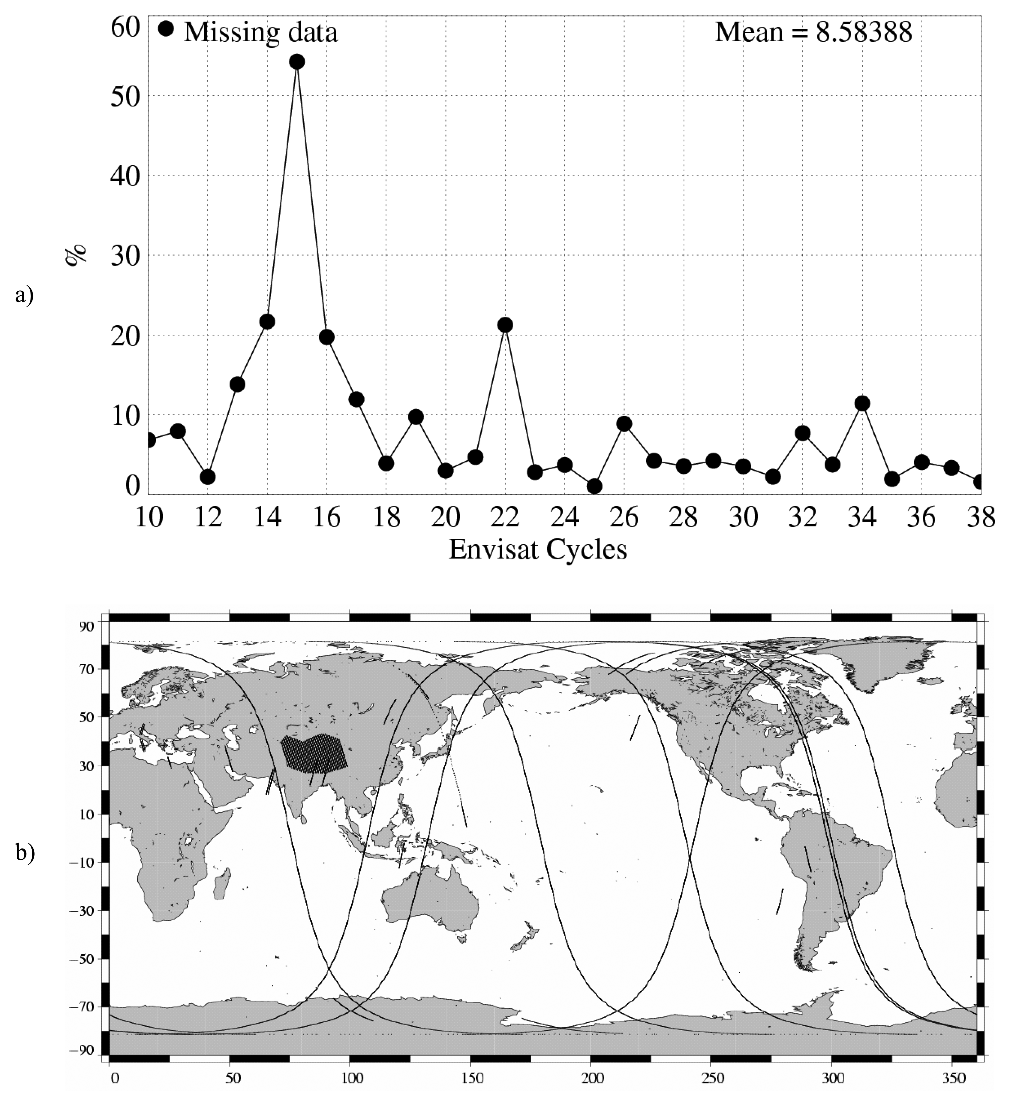
Figure 2.
Cycle by cycle percentages of missing MWR measurements.

Figure 3.
Cycle by cycle percentages of data impacted by the S-Band anomaly.
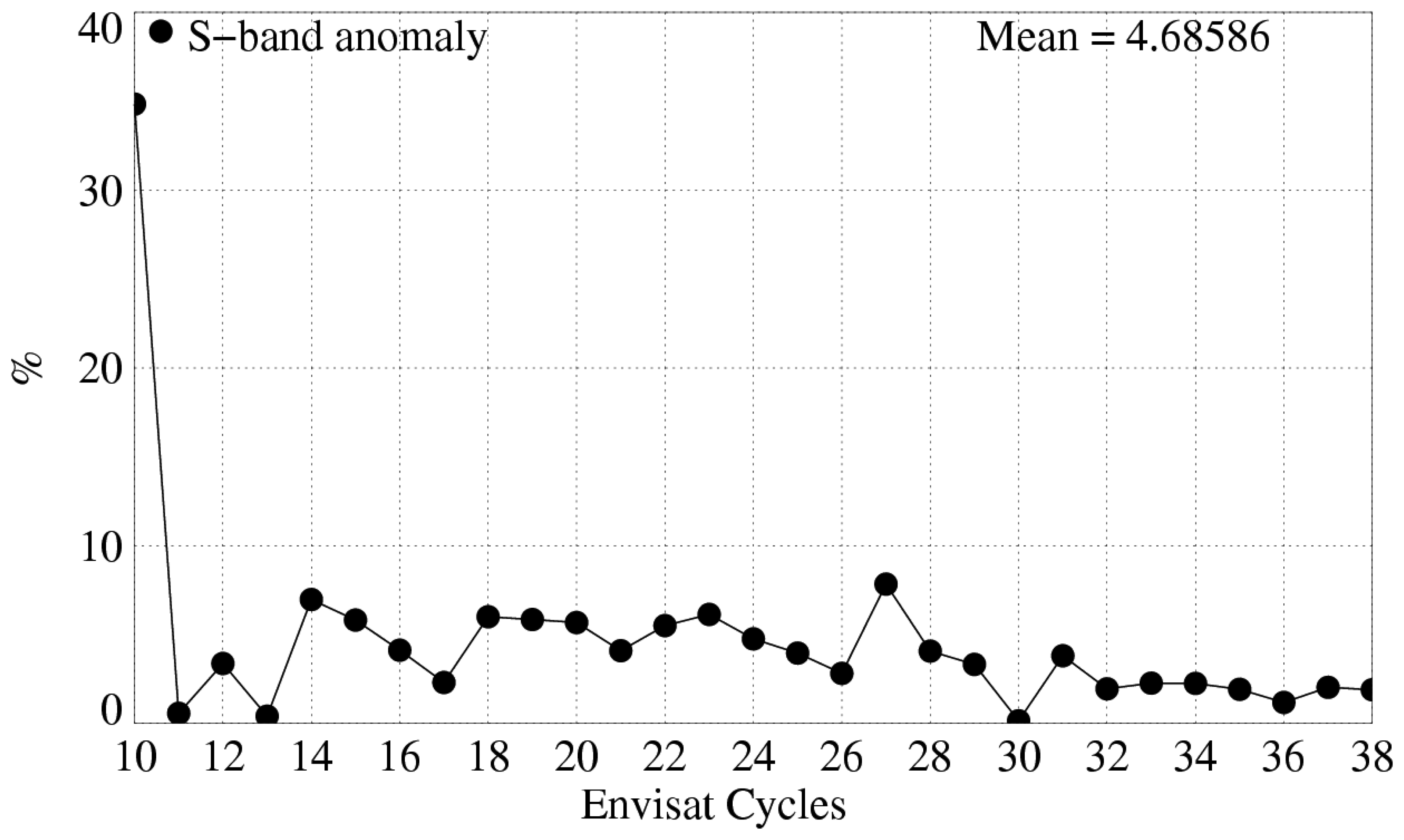
Figure 4.
Cycle per cycle percentages of edited measurements by the main Envisat altimeter and radiometer parameters: a) Standard deviation of 20 Hz range measurements > 25 cm, Number of 20-Hz range measurements < 10. b) Square of off-nadir angle (from waveforms) out of the [-0.2 deg2, 0.16 deg2] range. Dual frequency ionosphere correction out of [-40, 4 cm]. c) Ku-band significant wave height > 11 m, Ku band backscatter coefficient out of the [7 dB, 30 dB] range. d) MWR wet troposphere correction out of the [-50 cm, -0.1 cm] range. e) SSH-MSS out of the [-2, 2m] and edited using thresholds on the mean and standard deviation of SSH-MSS on each pass.
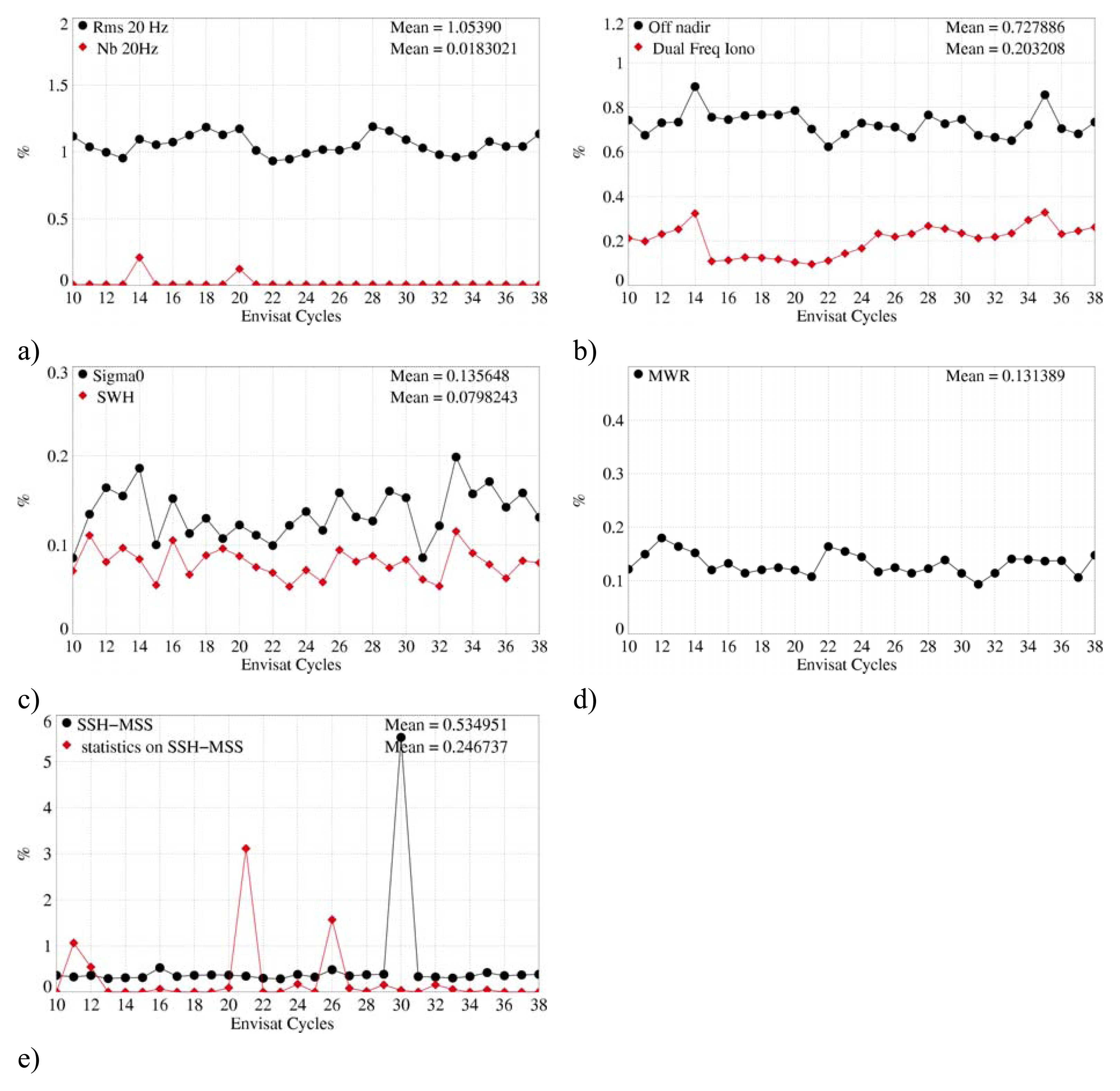
Figure 5.
Comparison of Envisat edited measurement to Jason-1. Maps of rejected measurements, with the same editing procedure for: a) 10 days of Envisat cycle 38 b) the corresponding Jason-1 cycle 128. c) Percentage of edited measurements, over ocean, for the two satellites, from the beginning of the Envisat mission.

Figure 6.
a) Cycle mean of the number of 20 Hz elementary range measurements used to compute 1 Hz range. b) Cycle mean of the standard deviation of 20 Hz measurements.
Figure 6.
a) Cycle mean of the number of 20 Hz elementary range measurements used to compute 1 Hz range. b) Cycle mean of the standard deviation of 20 Hz measurements.
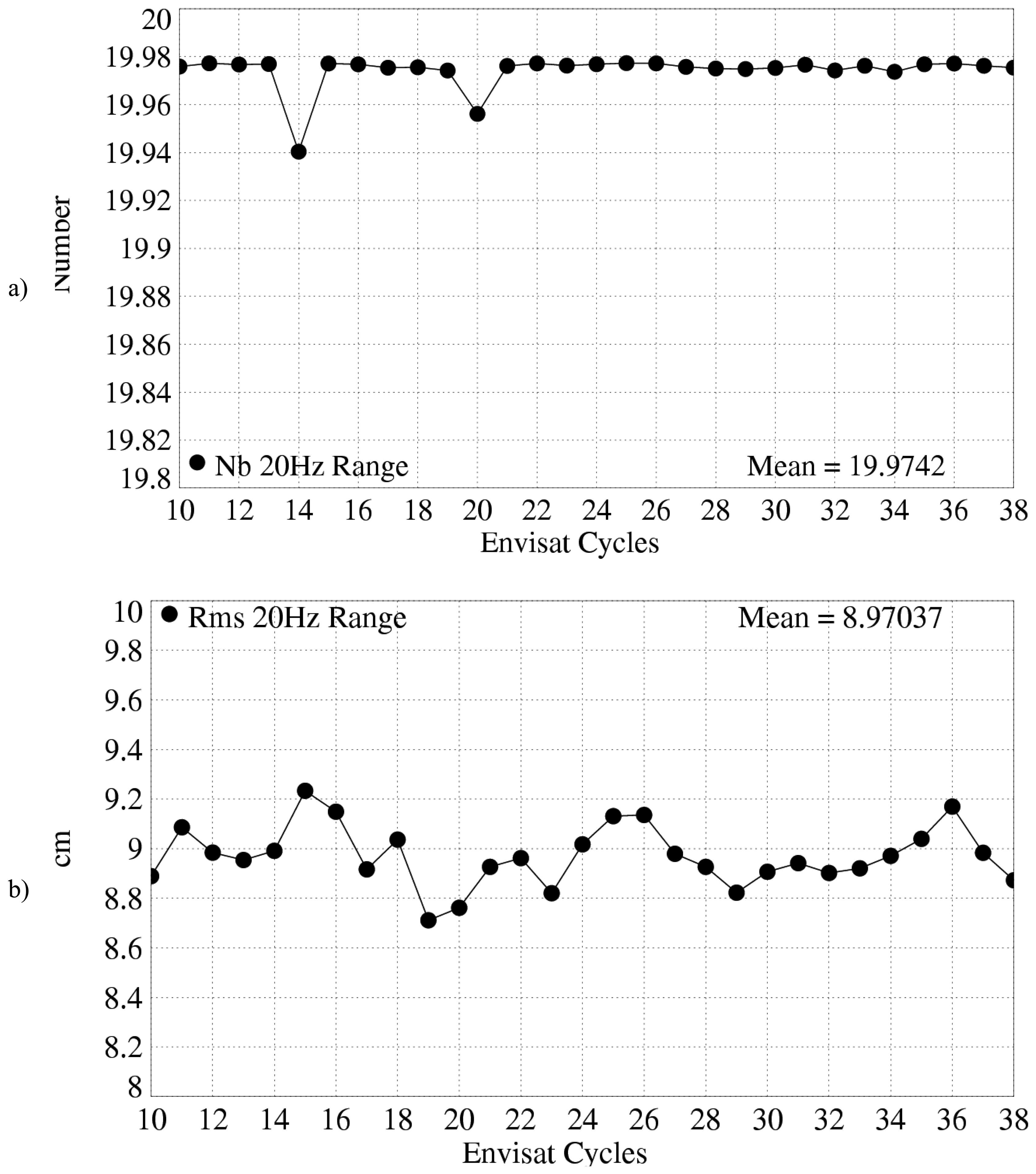
Figure 7.
Cycle mean of the square of the off-nadir angle deduced from waveforms (deg2).

Figure 8.
Global statistics (m) of Envisat Ku and S SWH a) Mean and b) Standard deviation. c) Mean Envisat-Jason-1 Ku SWH differences at 3h EN/J1 crossovers computed with 120 days running means. d) Mean. ERS-2-Envisat Ku SWH collinear differences over the Atlantic Ocean.
Figure 8.
Global statistics (m) of Envisat Ku and S SWH a) Mean and b) Standard deviation. c) Mean Envisat-Jason-1 Ku SWH differences at 3h EN/J1 crossovers computed with 120 days running means. d) Mean. ERS-2-Envisat Ku SWH collinear differences over the Atlantic Ocean.
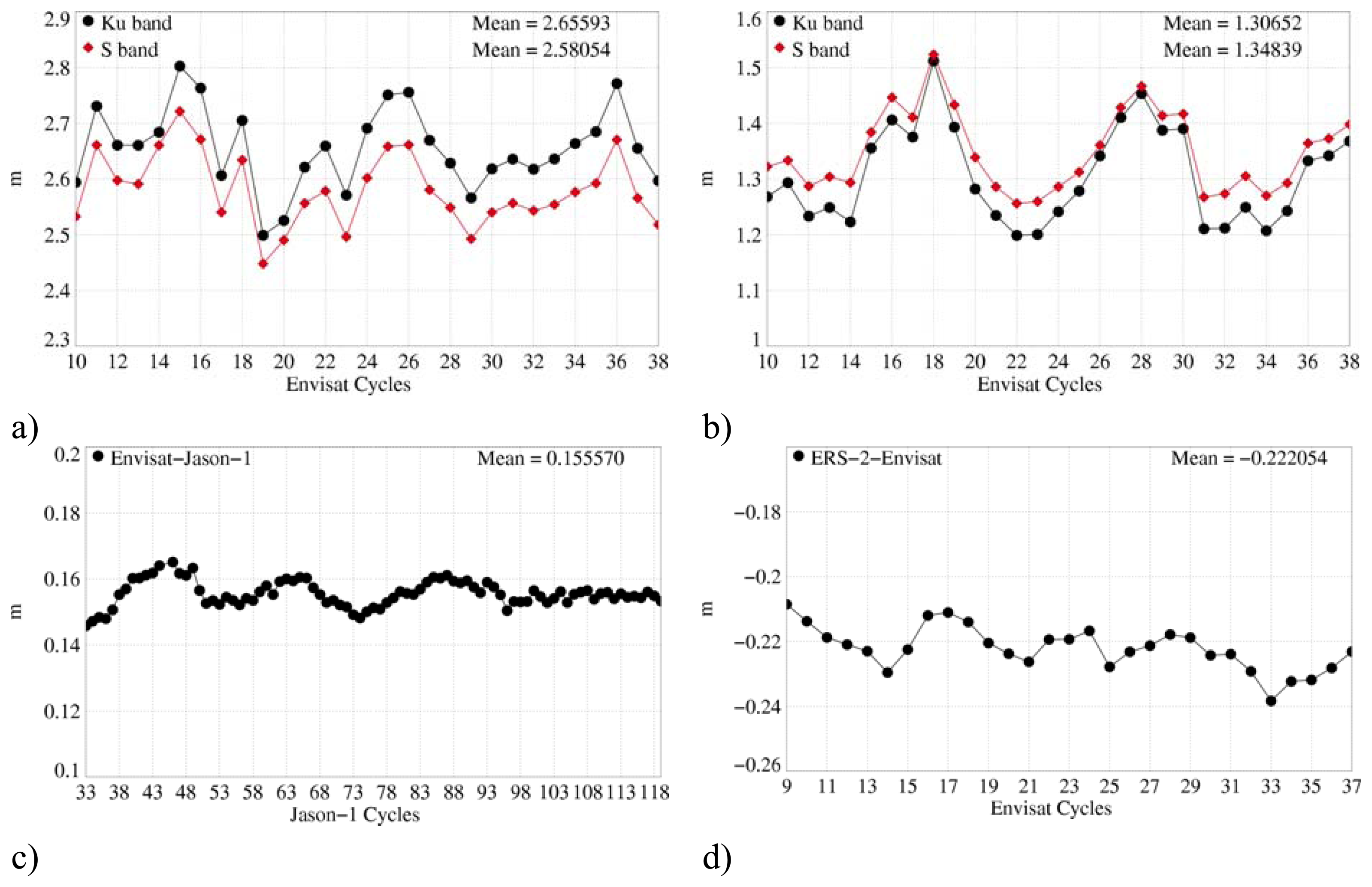
Figure 9.
Global statistics (dB) of Envisat Ku and S Sigma0 a) Mean and b) Standard deviation. c) Mean Envisat-Jason-1 Ku Sigma0 differences at 3h EN/J1 crossovers computed with 120 days running means. d) Mean ERS-2-Envisat Ku Sigma0 collinear differences over the Atlantic Ocean.
Figure 9.
Global statistics (dB) of Envisat Ku and S Sigma0 a) Mean and b) Standard deviation. c) Mean Envisat-Jason-1 Ku Sigma0 differences at 3h EN/J1 crossovers computed with 120 days running means. d) Mean ERS-2-Envisat Ku Sigma0 collinear differences over the Atlantic Ocean.

Figure 10.
Comparison of global statistics of Envisat dual-frequency and JPL-GIM ionosphere corrections (cm). a) Cycle mean of dual-frequency and GIM correction. b) Mean of the differences c) Standard deviation of the differences.
Figure 10.
Comparison of global statistics of Envisat dual-frequency and JPL-GIM ionosphere corrections (cm). a) Cycle mean of dual-frequency and GIM correction. b) Mean of the differences c) Standard deviation of the differences.
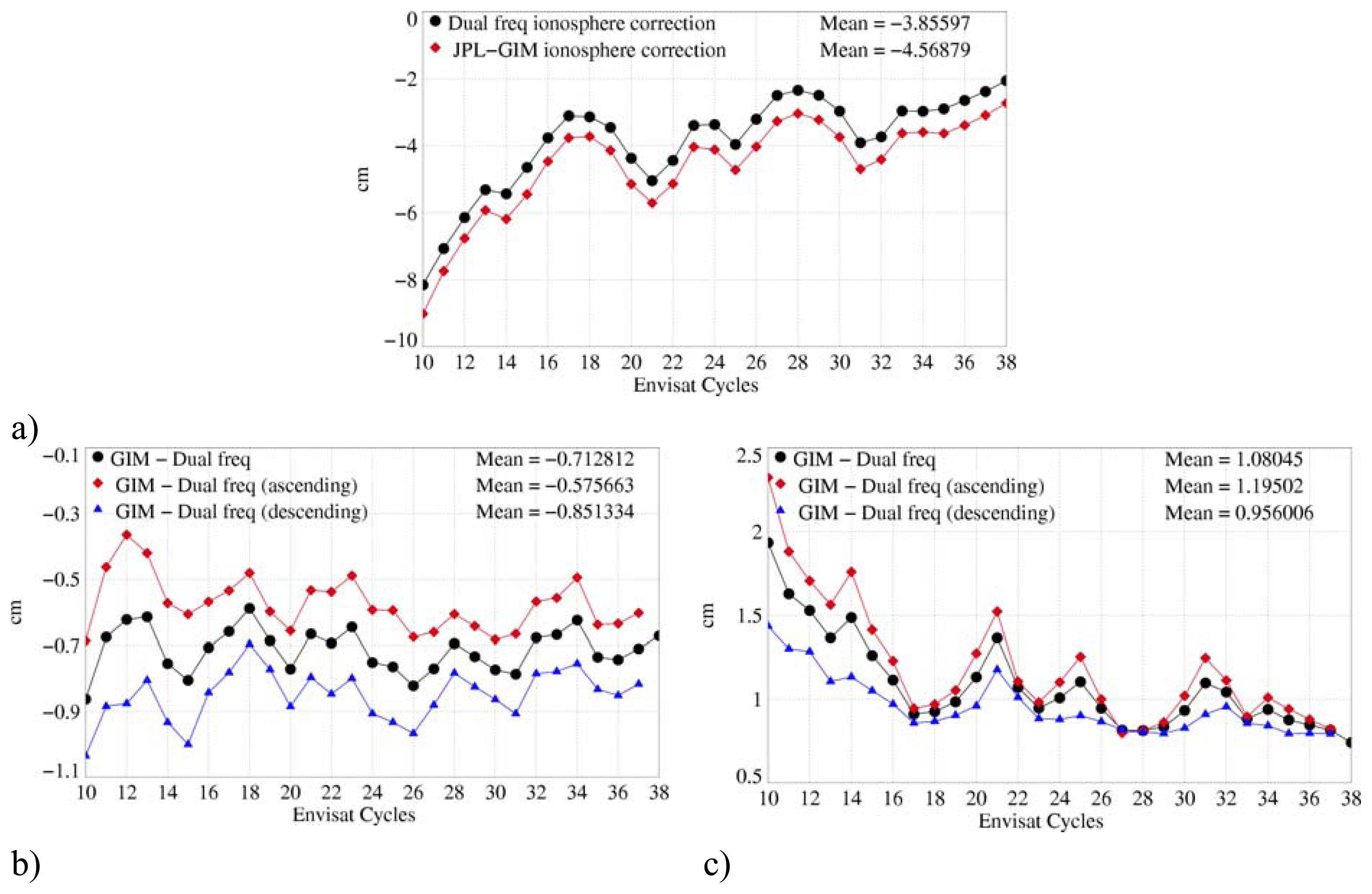
Figure 11.
Comparison of global statistics of Envisat MWR and ECMWF wet troposphere corrections (cm). a) Cycle mean of MWR and ECMWF corrections. b) Mean of the differences. c) Standard deviation of the differences.
Figure 11.
Comparison of global statistics of Envisat MWR and ECMWF wet troposphere corrections (cm). a) Cycle mean of MWR and ECMWF corrections. b) Mean of the differences. c) Standard deviation of the differences.
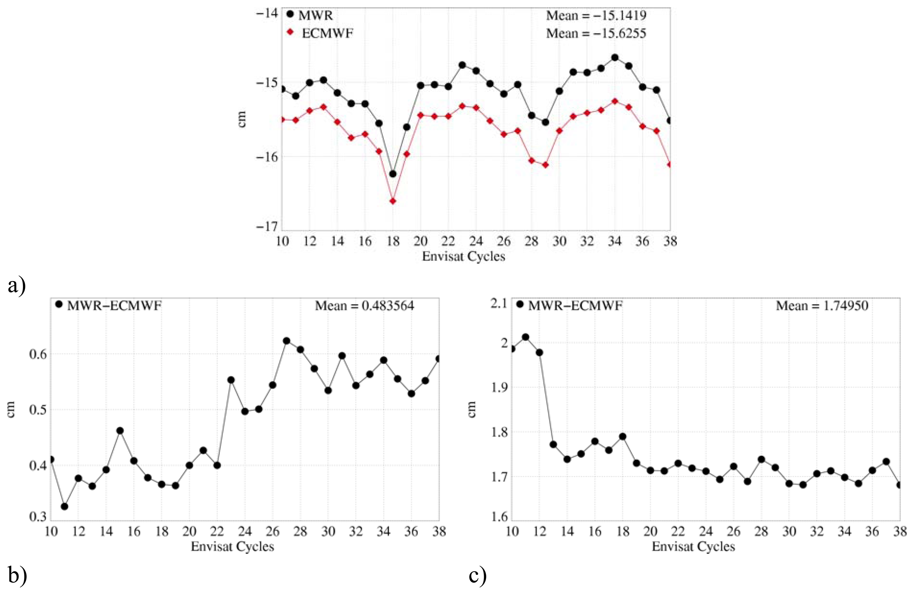
Figure 12.
Power spectrum of (a) 20 Hz Envisat SSH, (b) 20 Hz Jason-1 SSH, (c) 1 Hz Envisat SSH, (d) 1 Hz Jason-1 SSH.
Figure 12.
Power spectrum of (a) 20 Hz Envisat SSH, (b) 20 Hz Jason-1 SSH, (c) 1 Hz Envisat SSH, (d) 1 Hz Jason-1 SSH.
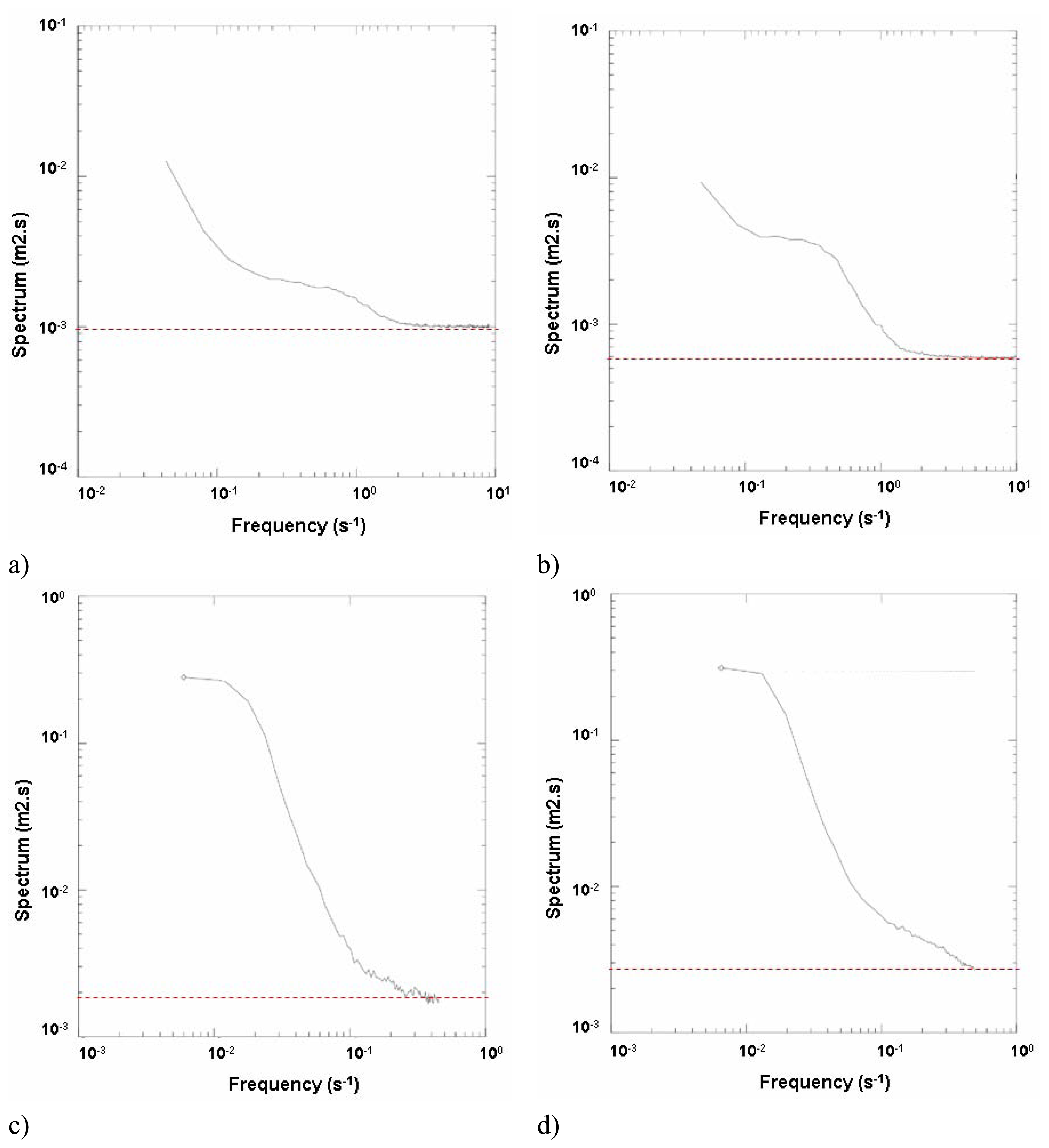
Figure 13.
Maps of the σ[HF(SSHJason-1-MSS]]- σ[HF(SSHEnvisat-MSS]] (cm) in (4deg × 4 deg) geographical bins through a 35-day period (cycle Envisat 23) where σ[HF(SSH-MSS;] is the standard deviation of the high frequency part of the SSH–MSS signal.
Figure 13.
Maps of the σ[HF(SSHJason-1-MSS]]- σ[HF(SSHEnvisat-MSS]] (cm) in (4deg × 4 deg) geographical bins through a 35-day period (cycle Envisat 23) where σ[HF(SSH-MSS;] is the standard deviation of the high frequency part of the SSH–MSS signal.
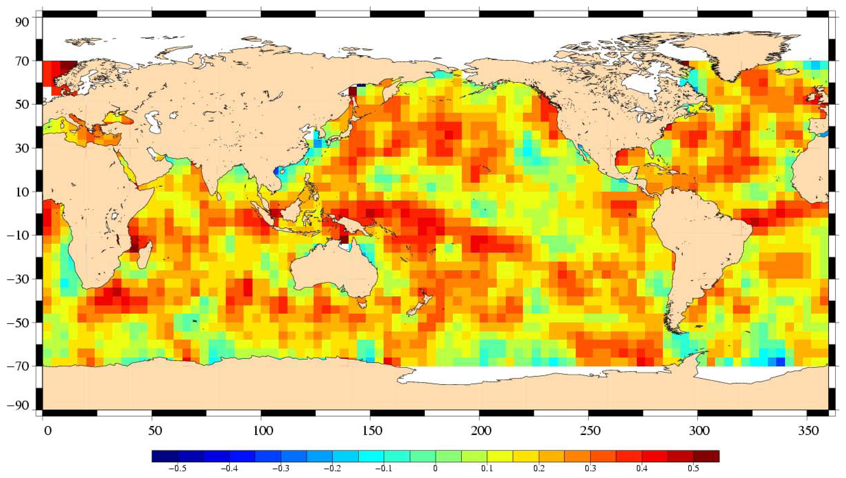
Figure 14.
Maps of the time invariant 35-day crossover mean differences (cm) for Envisat averaged in (4deg × 4 deg) geographical bins through a one year period (cycle 25-35) a) using GDRs POE orbit (GRIM5 gravity model) and b) using Delft POE orbit (EIGEN-GRACE01S gravity model;.
Figure 14.
Maps of the time invariant 35-day crossover mean differences (cm) for Envisat averaged in (4deg × 4 deg) geographical bins through a one year period (cycle 25-35) a) using GDRs POE orbit (GRIM5 gravity model) and b) using Delft POE orbit (EIGEN-GRACE01S gravity model;.
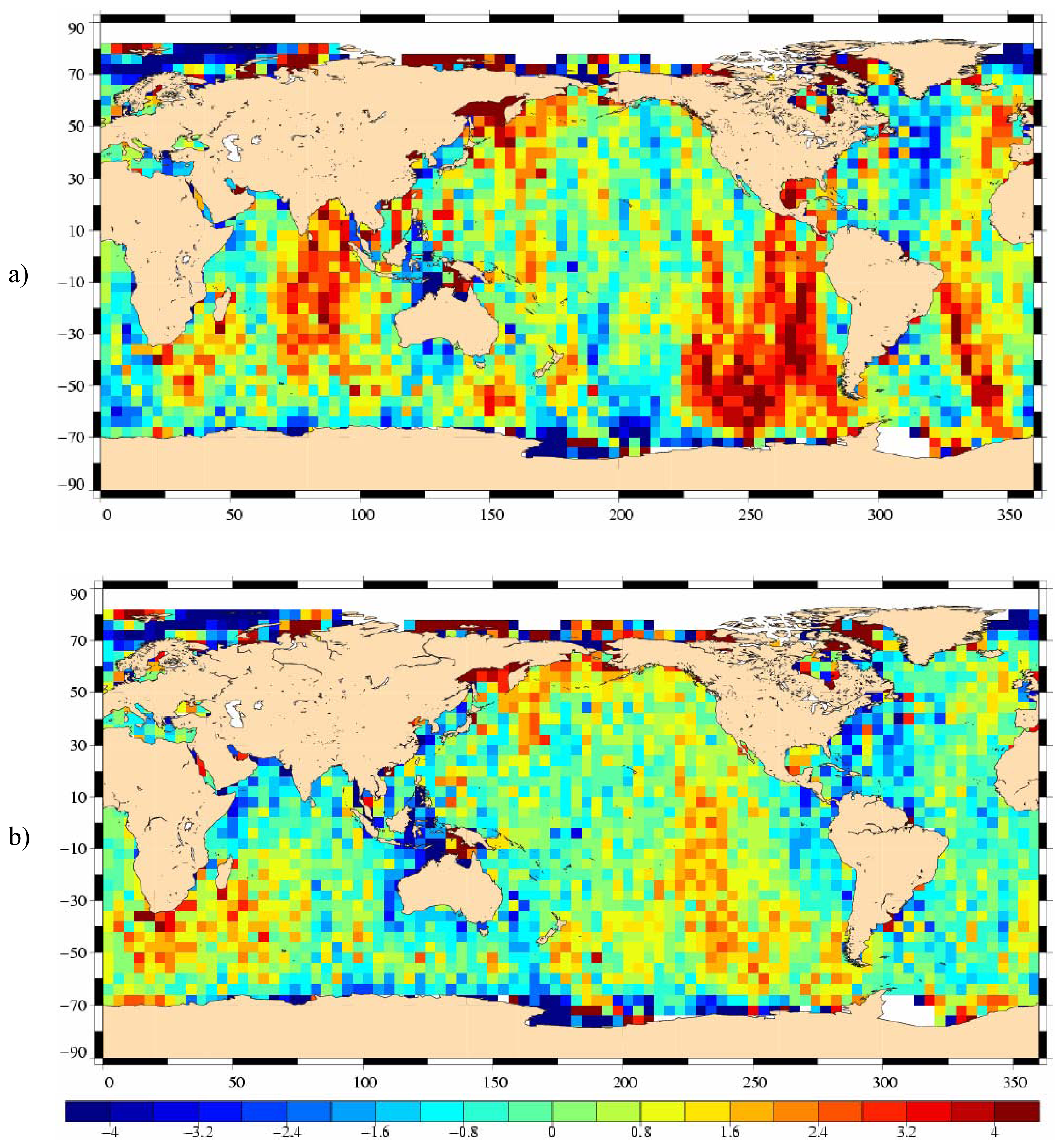
Figure 15.
Time varying 35-day crossover mean differences (cm). a) Cycle per cycle Envisat crossover mean differences. An annual cycle is clearly visible. Diamonds: shallow waters (1000 m) are excluded. Triangles: shallow waters excluded, latitude within [−50S, +50N], high ocean variability areas excluded b) Map of the geographic distribution of the amplitude of the annual cycle of the crossover means shown in a) averaged in 10deg × 10deg geographical bins (after smoothing).
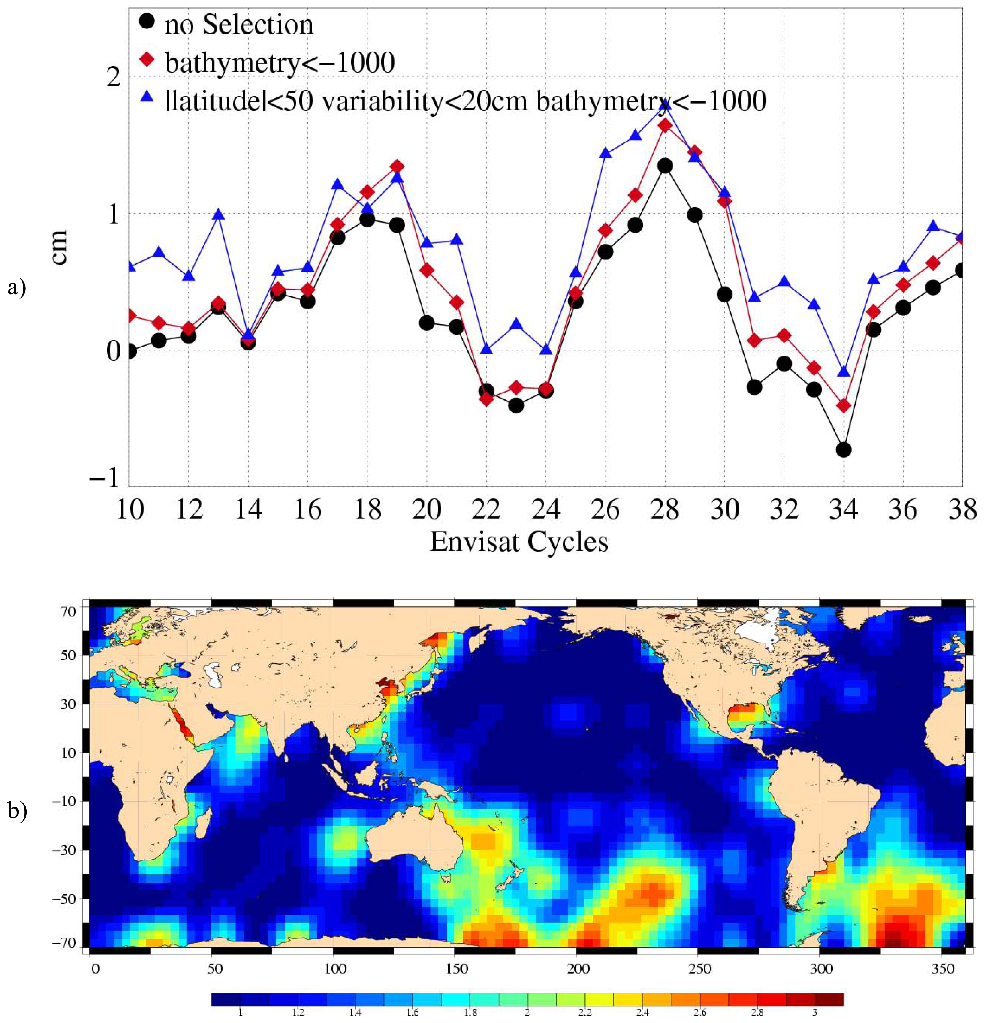
Figure 16.
a) Standard deviation (cm) of Envisat 35-day SSH crossover differences depending on data selection. Dots: without any selection. Diamonds: shallow waters (1000 m) are excluded. Triangles: shallow waters excluded, latitude within [−50S, +50N], high ocean variability areas excluded. b) Comparison of the Standard deviation (cm) of Envisat (dot) and Jason-1 (diamond) 10-day SSH crossover differences.
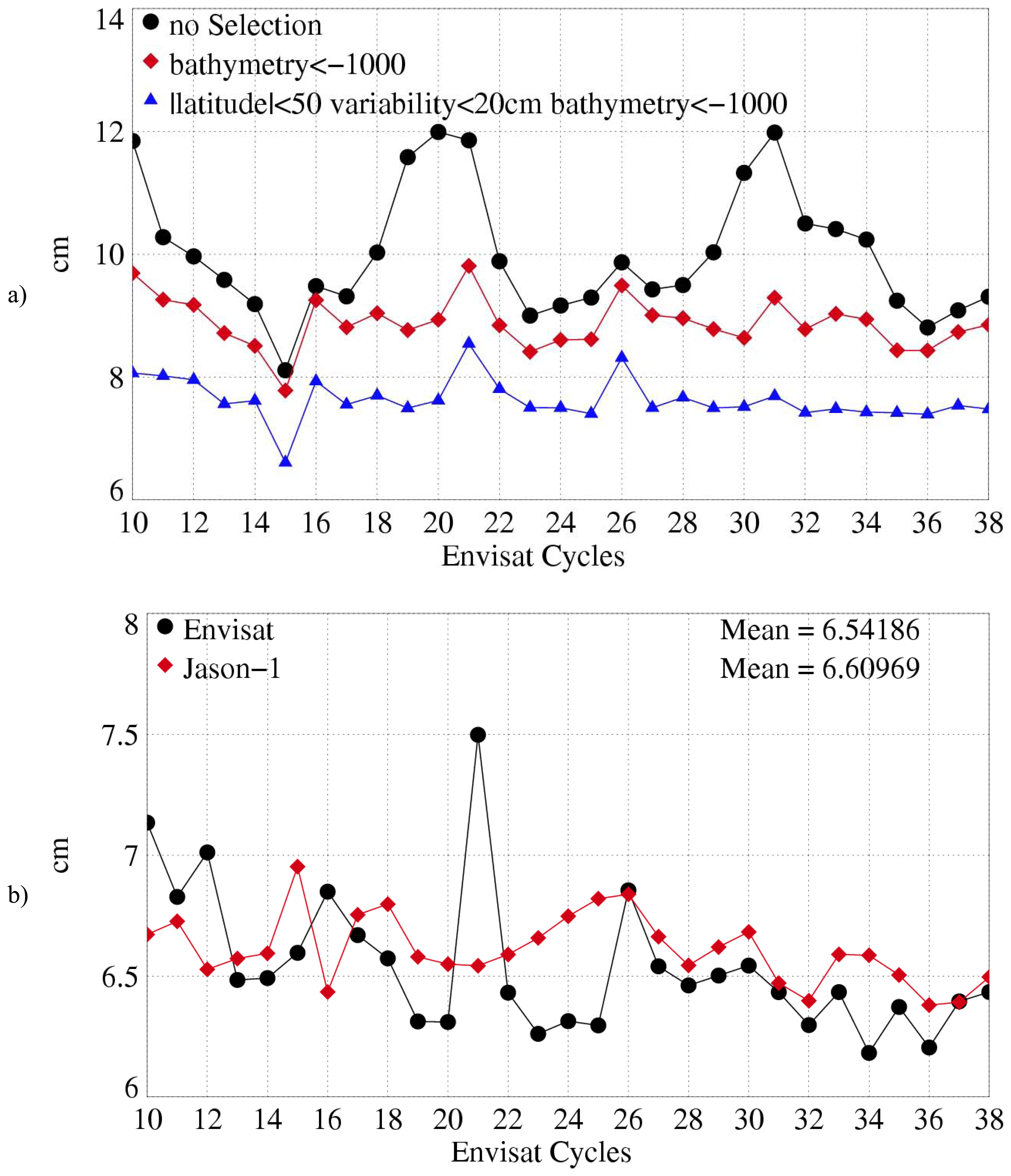
Figure 17.
USO correction computed from auxiliary files. The raw correction is averaged over 1 month.
Figure 17.
USO correction computed from auxiliary files. The raw correction is averaged over 1 month.

Figure 18.
Mean of Envisat sea level depending on data selection. Dots: without any selection. Diamonds: shallow waters (1000 m) are excluded. Triangles: shallow waters excluded, latitude within [−50S, +50N], high ocean variability areas excluded.
Figure 18.
Mean of Envisat sea level depending on data selection. Dots: without any selection. Diamonds: shallow waters (1000 m) are excluded. Triangles: shallow waters excluded, latitude within [−50S, +50N], high ocean variability areas excluded.
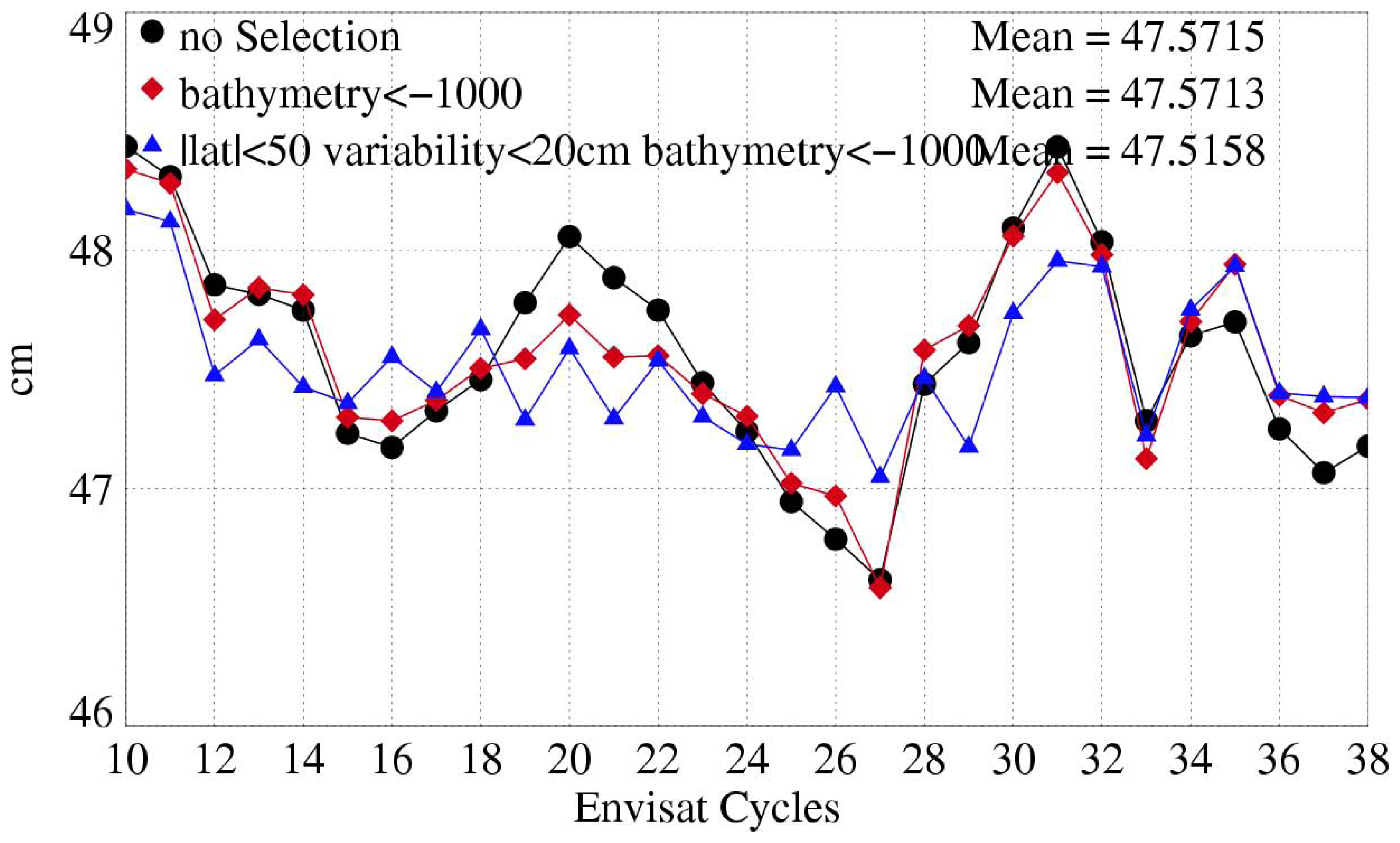
Figure 19.
Mean of Envisat –Jason-1 differences at 10-day dual crossovers. Dots: Global. Diamonds: Northern Hemisphere. Triangle: Southern Hemisphere.
Figure 19.
Mean of Envisat –Jason-1 differences at 10-day dual crossovers. Dots: Global. Diamonds: Northern Hemisphere. Triangle: Southern Hemisphere.
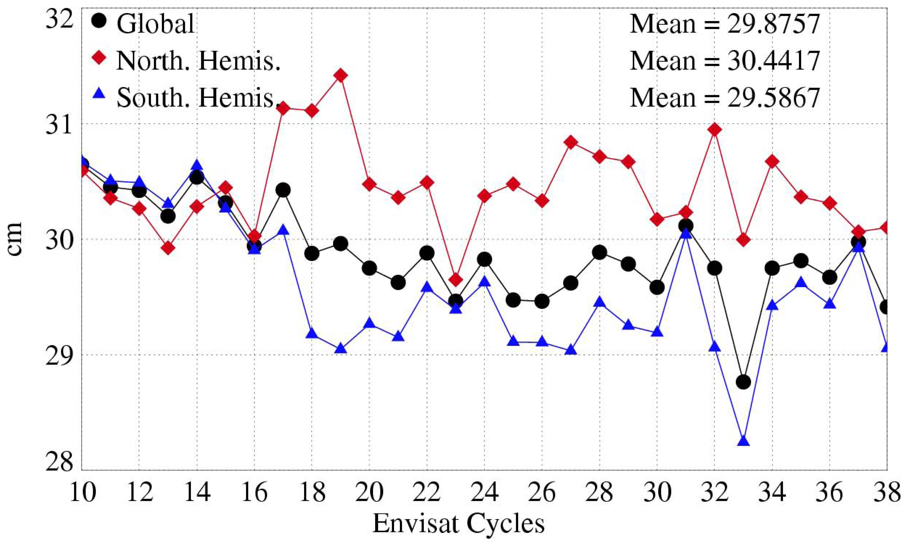
Figure 20.
Envisat, Jason-1 and T/P global MSL trends a) over the whole Envisat mission, b) over the two first years of Envisat mission (cycle 10 to 29), c) over the two last years of Envisat mission (cycle 19 to 38).
Figure 20.
Envisat, Jason-1 and T/P global MSL trends a) over the whole Envisat mission, b) over the two first years of Envisat mission (cycle 10 to 29), c) over the two last years of Envisat mission (cycle 19 to 38).
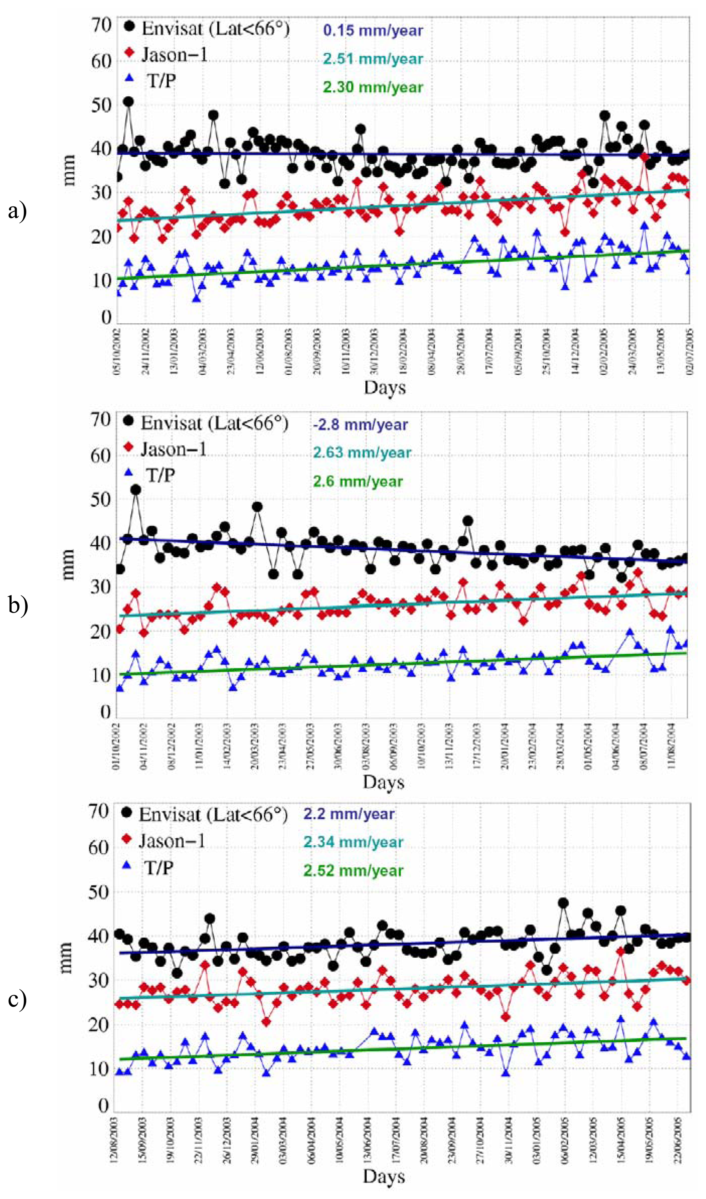
Figure 21.
Comparison of Envisat MSL to tide gauges. a) No USO correction applied and no long wave length error applied (dots), No USO correction applied and but a long wave length applied (diamonds); b) USO correction applied and a long wave length applied.
Figure 21.
Comparison of Envisat MSL to tide gauges. a) No USO correction applied and no long wave length error applied (dots), No USO correction applied and but a long wave length applied (diamonds); b) USO correction applied and a long wave length applied.


| Envisat | Jason-1 | T/P | |
|---|---|---|---|
| Orbit | CNES POE (grim5) | CNES POE (JGM3) | NASA POE (JGM3) |
| Additional Range correction | USO correction | none | none |
| SSB | Non parametric SSB (GDR) | Non parametric SSB (Labroue and Gaspar, 2002 [25]) | |
| Wet troposphere | For performance assessment: MWR For MSL estimation: ECMWF model, Gaussian grids | ||
| Dry troposphere | Based on ECMWF sea level pressure, rectangular grids | ||
| Ionosphere | Dual-frequency altimeter (filter 300km) | ||
| Inverse barometer | Based on ECMWF sea level pressure relative to global mean, rectangular grids | ||
| Tides | Pole tide, solid earth tide, GOT00.2 ocean and load tides | ||
| Mean sea surface | CLS01V1 | ||
© 2006 by MDPI ( http://www.mdpi.org). Reproduction is permitted for noncommercial purposes.
Share and Cite
MDPI and ACS Style
Faugere, Y.; Dorandeu, J.; Lefevre, F.; Picot, N.; Femenias, P. Envisat Ocean Altimetry Performance Assessment and Cross-calibration. Sensors 2006, 6, 100-130. https://doi.org/10.3390/s6030100
AMA Style
Faugere Y, Dorandeu J, Lefevre F, Picot N, Femenias P. Envisat Ocean Altimetry Performance Assessment and Cross-calibration. Sensors. 2006; 6(3):100-130. https://doi.org/10.3390/s6030100
Chicago/Turabian StyleFaugere, Yannice, Joël Dorandeu, Fabien Lefevre, Nicolas Picot, and Pierre Femenias. 2006. "Envisat Ocean Altimetry Performance Assessment and Cross-calibration" Sensors 6, no. 3: 100-130. https://doi.org/10.3390/s6030100