Improving the Response of a Load Cell by Using Optimal Filtering

Department of Circuits and Systems in the EUIT de Telecomunicacion at the Universidad Politecnica de Madrid (UPM), Campus Sur UPM, Ctra. Valencia km 7, Madrid 28031, Spain
Sensors 2006, 6(7), 697-711; https://doi.org/10.3390/s6070697
Submission received: 26 April 2006
/
Accepted: 28 July 2006
/
Published: 21 July 2006
(This article belongs to the Special Issue Intelligent Sensors)
Abstract
:Load cells are transducers used to measure force or weight. Despite the fact that there is a wide variety of load cells, most of these transducers that are used in the weighing industry are based on strain gauges. In this paper, an s-beam load cell based on strain gauges was suitably assembled to the mechanical structure of several seats of a bus under performance tests and used to measure the resistance of their mechanical structure to tension forces applied horizontally to the seats being tested. The load cell was buried in a broad-band noise background where the unwanted information and the relevant signal sometimes share a very similar frequency spectrum and its performance was improved by using a recursive least-squares (RLS) lattice algorithm. The experimental results are satisfactory and a significant improvement in the signal-to-noise ratio at the system output of 27 dB was achieved, which is a good performance factor for judging the quality of the system.
1. Introduction
Today's industry is experiencing a continuous positive change from obsolete technologies of measuring force or weight to the most advanced techniques that make use of the advances in microelectronics in order to incorporate a certain amount of intelligence into the sensors. What is more, the soaring need for both better quality and reliability of the products we fabricate, and better comfort and safety in today's processing plants, has set a revolutionary way of designing sensors and transducers for industrial applications. Smart sensors (or intelligent transducers), which consist of sensors, analog signal conditioners, analog-to-digital converters, microprocessors, digital signal processors and other integrated circuits, have transformed the sensors into robust and optimal measuring systems that are able to work satisfactorily in polluted environments.
In fact, one of the worst environments for sensors and transducers is that of the automotive industry. In such an environment, sensors and transducers have to endure dangerous chemical attacks, undesirably strong vibrations, electromagnetic interferences, high temperatures, high humidity, noise coming from other electromechanical machines, and so on. Therefore, with this scenario in mind, no one would dispute that the robustness, efficiency and reliability of the sensors and transducers have been, and will continue to be, crucial.
This paper shows the improvement of the real-time response of a load cell used to carry out the measurement of tension forces applied horizontally to the mechanical structure of several seats of a bus under performance tests. In short, in a car crash the seats cannot detach themselves from their supports. This is a safety-related problem.
2. Load cells
Among the complete family of sensors and transducers for automotive, research, consumer and industrial applications, load cells stand out as one of the most important transducers. Basically, these transducers measure deformations produced by force or weight [1]. In addition, according to the type of output signal they generate and the way they detect the weight, there are many types of load cells, for instance: strain gauge cells, mechanical cells, and other types (fibre optic, piezoresistive, and so on). However, due to their high accuracy and low cost, strain gauge load cells are the most used in today's industry. Most of today's load cell designs use strain gauges as the sensing element.
Depending on the application, strain gauges can be either metal or semiconductor strain gauges. The latter ones are made of semiconductor materials, particularly silicon, but have advantages and disadvantages.
On the one hand, semiconductor strain gauges are very small and have large gauge factors. In fact, resistance changes here are much bigger than those obtained with metal strain gauges. They are frequently used in designing miniature load cells.
On the other hand, the resistance versus strain curve of these devices is highly nonlinear. Therefore, when using semiconductor strain gauges, we must have a curve or table of values of gauge factor versus resistance [1]. What is more, the signal conditioning circuit should include linearization stages in order to carry out the linearization of the output voltage.
Generally speaking, they are usually placed in a Wheatstone bridge circuit to measure the resistance changes in the strain gauges. Furthermore, depending on the number of active strain gauges used in the bridge configuration such a configuration is called a one-arm bridge, a two-arm-bridge or a four-arm bridge.
In this paper, the strain sensors used were metal strain gauges with nominal resistance 350 Ω, and suitably wired in a four-arm bridge configuration. In such a configuration, two of the gauges are usually in tension and two in compression, and wired with compensation adjustments. Figure 1 shows the typical one-arm bridge configuration.
In figure 1, supposing that R1 = R2 = R3 = R, which is the nominal gauge resistance, and that the active strain gauge resistance is given by
where (ΔR/R) is the fractional change in gauge resistance because of strain, then the bridge off-null voltage will be given by
where (ΔR/R ) ≪ 1, GF stands for the gauge factor, and (Δl/l) is the fractional change in length. In addition, GF is approximately equal to 2 for metals and as large as 10 for some special alloys and carbon gauges [1]. Furthermore, for silicon, GF is approximately 100 to 200, depending on the doping level and the design [2,3].
For the two-arm bridge configuration, the bridge off-null voltage is given by
For the four-arm bridge configuration, the bridge off-null voltage is given by
Here, it is important to say that there is large number of load cell types. For instance, for industrial applications, among the most used load cell types, we can mention the following: bending beam, shear beam round, shear beam rectangular, miniature, low profile, ‘s’ or ‘z’ beam, canister, compression/tension, compression, and platform and single point load cells. Furthermore, for the automotive industry, among the most used load cell types, we can also mention the following: seat belt, gear stick, steering wheel, pedal force and in-line suspension load cells.
The load cell used in this paper was an s-beam load cell with a rated capacity of 20 kN. The s-beam load cell is a load cell where the structure is shaped as a ‘S’ or ‘Z’ and strain gauges are bonded to the central sensing area in the form of a full Wheatstone bridge.
The load cell was calibrated by the National Accreditation Body of Spain and the result of the calibration was an uncertainty of ± 0.38% of full-scale output. This uncertainty estimate represents an expanded uncertainty expressed at approximately the 95% level of confidence using a coverage factor of k = 2.
3. Optimal filtering
Due to the many sources of noise that corrupt the information coming from the sensors and transducers used in industrial applications and the little knowledge we have of the noise characteristics, it is very difficult to cancel the unwanted information that corrupts the relevant signal without causing damage to the relevant signal itself. The more the noise and the relevant signal share the same (or a very similar) frequency spectrum, the less the designer can remove the unwanted information by using classical filtering techniques [4-8]. What is more, if the signal of interest and/or the noise are not stationary processes, which is the case under study, the use of a Wiener filter [9] is inadequate [10-16].
In the present paper, the information coming from the load cell was corrupted by electrical and mechanical noise. In the performance tests carried out in the laboratory, the noise corrupting the relevant information came from many sources. Examples of such noise sources are the following: mechanical vibrations of electromechanical machines, noise of the servovalves and the actuators, electromagnetic interferences, electrical noise, and noise of the computer, the monitor, the fluorescent lights, the alternators, the electrical distribution system, and the heating, ventilation and air conditioning systems, among others.
The load cell was buried in a broad-band noise background where the unwanted information and the relevant signal sometimes share a very similar frequency spectrum. For this reason, it was necessary to use a self-designing system with the ability to perform satisfactorily in an environment where complete knowledge of the relevant signal characteristics is not available (i.e., an adaptive filter) [17-21].
According to Hernandez [15], an adaptive filter is a filter with a mechanism for adjusting its own parameters automatically by using a recursive algorithm at the same time that it is in active interaction with the environment. All this happens in such a way that the performance of the adaptive filter is continuously improved according to a specified performance criterion (or cost function) which has been previously established by the designer.
In accordance with [20], there is a wide variety of recursive algorithms used to design adaptive filters, but the choice of an algorithm over another is determined by the following factors:
- Satisfactory rate of convergence
- Misadjustment
- Tracking
- Robustness
- Low computational burden
- Good numerical behaviour
- Good round-off error rejection
- The structure of information flow in the algorithm
Taking into consideration the above statements, in this paper, a recursive least-squares (RLS) lattice adaptive filter was chosen to carry out the optimal estimation process of the relevant signal [15,16,20-23]. Here, the application of such an adaptive filter is an interference or noise canceller [18,20].
Figure 2 shows a block diagram representation of the adaptive noise canceller. In figure 2, the transfer function H is used to show that the signals from the noise sources are uncorrelated with the relevant signal but correlated in some way with the noise of the relevant signal. A summary of the RLS lattice algorithm is given in the next subsection.
3.1. Summary of the RLS lattice algorithm (from Haykin [20] and Hernandez [15,16])
According to Haykin [20], the RLS lattice algorithm is based on a priori estimation errors, and the reflection and joint-process estimation coefficients are all derived directly. The algorithm is called the RLS lattice algorithm using a priori estimation errors with error feedback. Additional information about the ways to derive this algorithm and its advantages and disadvantages can be found in [15,20,21].
3.1.1. The RLS lattice algorithm using a priori estimation errors with error feedback
3.1.1.1. Initialization
To initialize the algorithm, at time n = 0, set
where δ is a small positive constant, Φ is the forward prediction-error energy, Θ is the backward prediction-error energy, r is the order of the least-squares predictor and r = 1, 2, …, R0, where R0 is the final order of the least-squares predictor. In addition, γ is the forward reflection coefficient, π is the backward reflection coefficient, and κ is the conversion factor.
For each instant n ≥ 1, generate the zeroth-order variables:
where the constant λ, 0 < λ ≤ 1, is the forgetting factor and its typical values used are the real numbers in the range from 0.99 to 1, η is the forward a priori prediction error, β is the backward a priori prediction error, and x is the reference input.
For joint-process estimation, at time n = 0, set
where σ is the tap-weight vector of the transversal filter. It contains R0 + 1 taps.
At each instant n ≥ 1, generate the zeroth-order variable
where y is the primary input and ε is the system output.
3.1.1.2. Predictions
For n = 1, 2, 3, …, compute the various order updates in the sequence r = 1, 2, …, R0.
3.1.1.3. Filtering
For n = 1, 2, 3,…, compute the various order updates in the sequence r = 1, 2, …, R0 + 1:
Before moving on to the results of the experiment, it is important to point out that the output of the filtering process (εR0+1) is the system output (see figure 2). Moreover, the outputs of the lattice predictor (ηR0 and βR0) are the variables used in this paper to obtain the cost function (see Section 4).
4. Results of the experiment
In this paper, one end of the s-beam load cell was assembled to a computer-controlled hydraulic cylinder and the other end was suitably assembled to the mechanical structure of each seat being tested in each experiment. Then, a dummy load cell was used to provide information about the noise corrupting the relevant signal coming from the active load cell (i.e., the reference input, see figure 2). Specifically, the dummy was mounted in an insensitive position, but close to the active load cell. Therefore, both transducers were affected by the same (or very similar) noise, but only the active load cell was used to measure the tension force applied horizontally to the seats being tested in each experiment. Experience tells us that part of the noise of the primary input (see figure 2) is correlated in some way to the noise coming from the dummy.
At this point, some important facts should be stressed:
- First, the frequency bands of the relevant signal and the unwanted signals overlap; they are mixed with each other. In short, the frequency band of the noise generated by the mechanical vibrations lie in the low frequency range.
- Second, if magnetic fields are present, mechanical vibrations can generate electrical interference.
- Third, capacitance changes associated with vibrating wires generate unwanted interference signals.
- Fourth, the frequency band of the electrical noise generated by computers, monitors, alternators, fluorescent lights, motors, and so on, ranges from several Hertz to several kilo Hertz.
- Last of all, the electronic noise corrupts the important information in its entire frequency band. Such a noise is generated by the electronic systems, discrete components (i.e., diodes, resistors, transistors, etc…), operational amplifiers, signal conditioning circuits, hardware, data acquisition cards, and soon.
4.1. Filtering
After studying the bandwidth of the relevant signal, a sampling frequency of 100 Hz was chosen. The signal treatment was carried out by using a laptop computer and the National Instruments Data Acquisition Card DAQCard-700. Nine experimental tests were carried out under laboratory conditions.
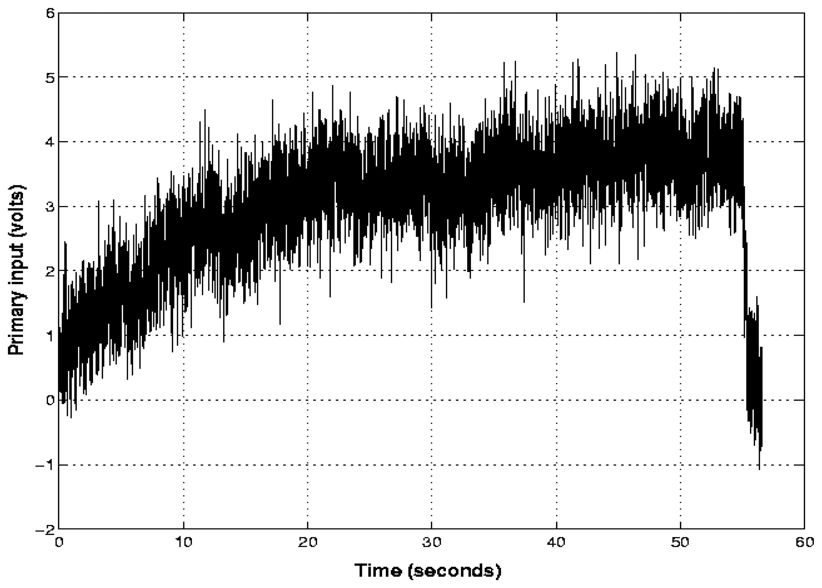
Figure 3 shows the information coming from the transducer and the analog signal conditioning stage (i.e., the primary input) in one of the experimental tests.
Furthermore, the mean-squared error (i.e., the cost function) of the filter is
where E is the expectation operator, and figure 4 shows the normalized mean-squared error of the filter over the nine independent trials of the experiment. The cost function shown in figure 4 is normalized with respect to the infinite norm of the vector consisting of the nine independent trials of the experiment.
The independent trials were carried out in the following way: 1 independent trial was done for each one of the 9 possible combinations of the variables shown in figure 4. In figure 4, the values of the length (or number of taps) of the filter (R0 + 1) are the following: 10, 50 and 100. Also, the values of the forgetting factor (λ) are the following: 0.995, 0.999 and 1.
What is more, the values of R0 were chosen in accordance with the idea of implementing an adaptive filter with a small number of adaptive weights, and experience tells us that the values of λ should be in the range from 0.99 to 1.
According to Hernandez [15,16], if λ is lower than 0.99, the system is numerically unstable. In short, if λ is lower than 0.99, the system has poor numerical behaviour, i.e. it becomes numerically inaccurate, and works with inaccurate values of the forward and backward reflection coefficients (see subsection 3.1). Then, the positive definiteness of the underlying inverse correlation matrix of the input data is lost. Therefore, the system does not converge and its output starts to oscillate in an uncontrollable manner.
According to Hernandez [16], it is also important to point out that the designer may use a large number of taps of the filter. But doing so could cause problems due to weight-vector noise. Specifically, a large number of taps could increase the difference between the ensemble-average value of the tap-weight vector and the tap-weight vector (such a difference is called the weight-vector noise). This increment makes the figures of merit for assessing the tracking capability of the RLS lattice adaptive filter worse. Such figures of merit are the estimation variance and the misadjustment of the adaptive filter.
The above problems diminish the detection ability of the relevant signal due to spurious peaks, which may be confused with the important signal.
Taking into consideration the above statements and the information shown in figure 4, in this paper the length of the RLS lattice adaptive filter and the forgetting factor were chosen to be 50 and 1, respectively. Also, it is important to highlight that the closer λ is to 1, the better the performance of the RLS lattice adaptive filter is. However, it is wrong to think that the larger the number of taps of the adaptive filter, the better the filter is. High-order filters increase the computational burden and therefore the speed of the required processor. What is more, they require increased software complexity, which increases coding and debugging time [20].
Therefore, for each specific application, it is suggested that the designer tests the performance of the RLS lattice adaptive filter for several values of number of taps of the filter and forgetting factors before making his/her final choice [15,16].
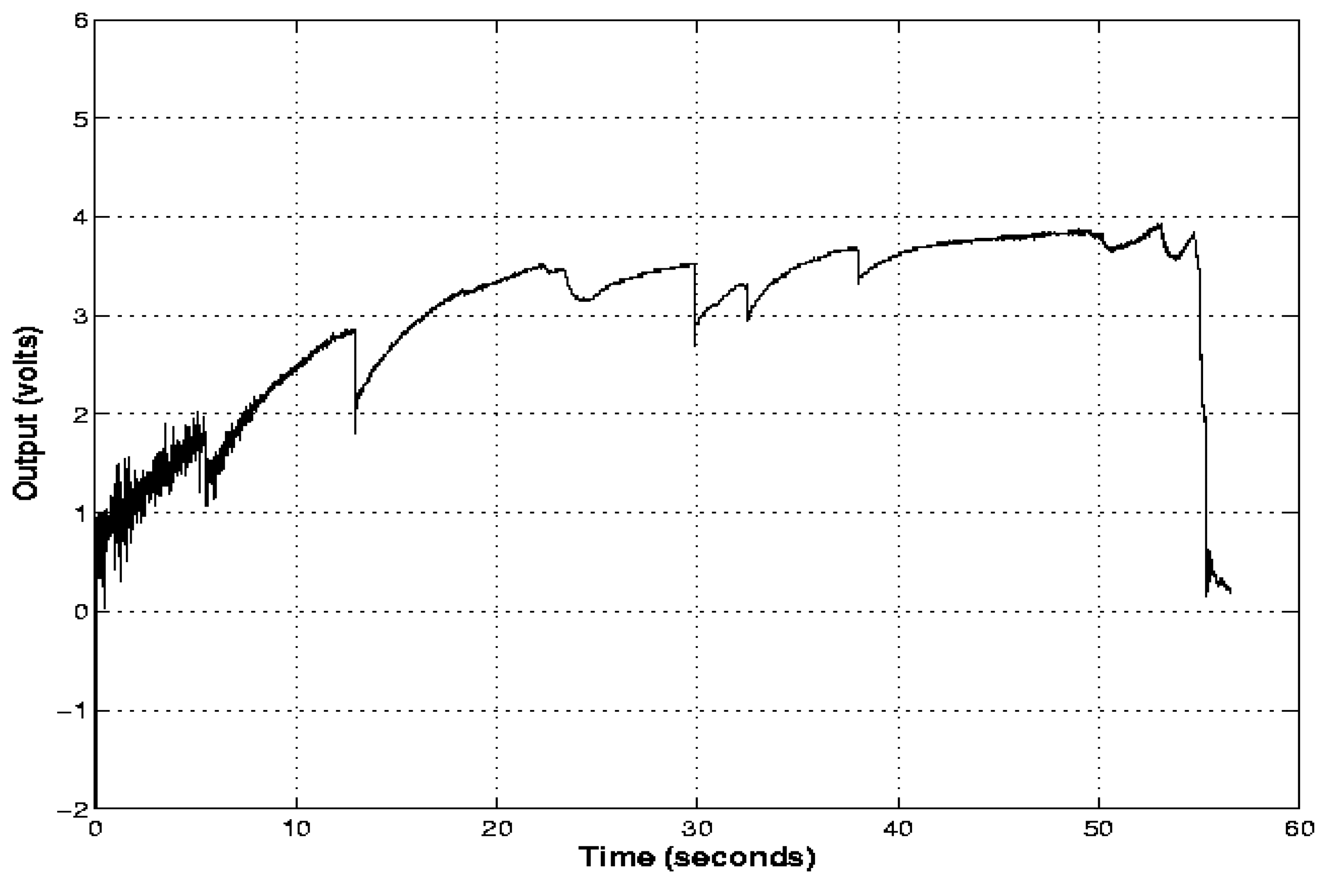
Figure 5 shows the output of the system and figure 6 shows the power spectrum magnitude of both the primary input (see figure 3) and the system output (see figure 5). In figure 5, it can be seen that the adaptive noise canceller significantly reduced the noise corrupting the relevant information while leaving the important information relatively unchanged from a practical viewpoint. In addition, it can be seen the whole process of testing the resistance of the mechanical structure of the seat being tested in one of the experiments carried out in the laboratory to a tension force applied horizontally to the seat. This figure shows clearly the time domain performance of the mechanical structure of the seat to several step inputs in reference from 5kN to 20kN. The seat being tested in this experiment detached itself from its supports at 20kN, which is a very good performance.
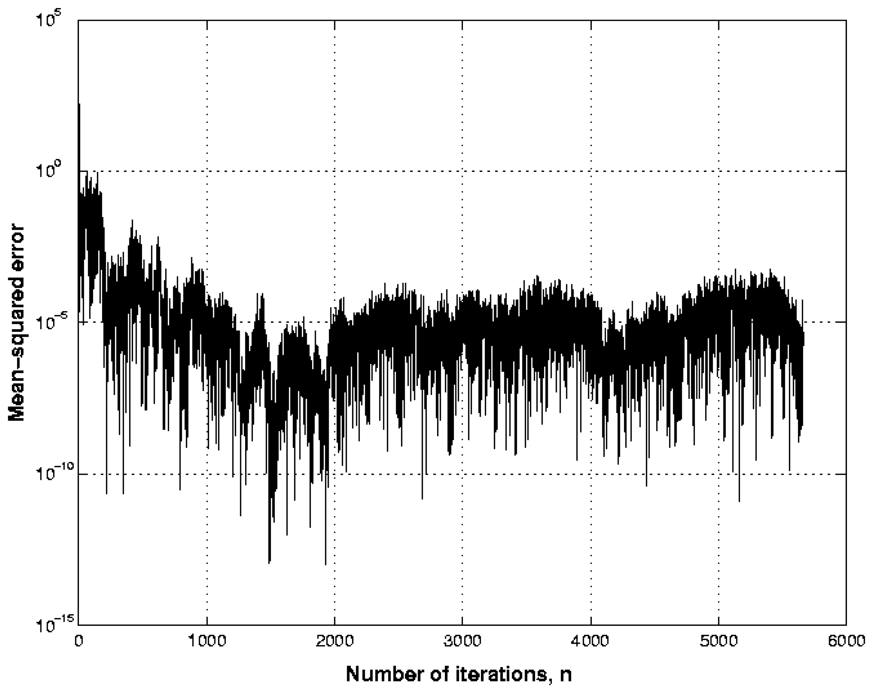
In the present paper, the signal-to-noise ratio (SNR) of the primary input (see figure 3) is approximately 16 dB, and the SNR at the system output (see figure 5) is approximately 43 dB. Therefore, a SNR improvement of approximately 27 dB was achieved, which is a good performance factor for judging the quality of the filter. Furthermore, the learning curve for the RLS lattice adaptive filter presented in this paper is shown in figure 7, which is also a satisfactory result. In short, this figure shows an experimental plot of the learning curve of this paper's adaptive filter and it was obtained by ensemble-averaging the squared error of the adaptive filter over 9 independent trials of the experiment.
Before going on to the conclusions, it is important to highlight that there are many other techniques of both analog signal conditioning and digital signal conditioning [1,24-34] that can also give satisfactory results under certain conditions But when the sensors and transducers are buried in a broad-band noise background like the one shown in this paper, only by the fusion of robust and optimal signal processing techniques with microcontroller units, digital signal processors and application specific integrated circuit technologies can the designer find the appropriate way to build the intelligent (or smart) sensors that today's industry needs.
5. Conclusions
This research was part of a study of the performance of the seats of a bus during its fabrication process. The results allowed us to satisfactorily estimate the information coming from the load cells used in the performance tests without the necessity of buying expensive precision electronic instrumentation.
In this paper, the RLS lattice adaptive filter was used to improve the performance of a load cell used to measure tension forces applied horizontally to the mechanical structure of several seats of a bus under performance tests. This kind of test is very important for car manufacturers. In a car crash the seats cannot detach themselves from their supports. This is a safety-related problem.
The experimental results are satisfactory, and a SNR improvement of 27 dB was achieved. These results are a good performance factor for judging the quality of the filter.
In addition, the optimal system presented in this paper was built by using low-cost components. The cost of the electrical components of the design was 12 US dollars. This is a very important factor to be taken into consideration when fabricating the sensors and transducers that today's industry needs. What is more, this factor makes the use of the technique presented in this paper affordable for intelligent sensor manufacturers.
This paper's design method can contribute positively to bridge the gap between intelligent signal processing methods and the design of intelligent sensors for automotive, research, consumer and industrial applications.
Acknowledgments
This work was supported by the Department of Circuits and Systems in the EUIT de Telecomunicacion at the Universidad Politecnica de Madrid, Spain.
References
- Johnson, C. D. Process control instrumentation technology, Fifth Edition ed; Prentice-Hall, Upper Saddle River: New Jersey, 1997. [Google Scholar]
- Shankland, E. P. Piezoresistive silicon pressure sensors. SENSORS MAGAZINE 1991, 22, 22–26. [Google Scholar]
- Frank, R. Understanding smart sensors, Second Edition ed; Artech House: Norwood, MA, 2000. [Google Scholar]
- Kalman, R. E. A new approach to linear filtering and prediction problems. Trans. ASME, J. Basic Eng. 1960, 82, 35–45. [Google Scholar]
- Kalman, R. E.; Bucy, R. S. New results in linear filtering and prediction theory. Trans. ASME, J. Basic Eng. 1961, 83, 95–107. [Google Scholar]
- Sorenson, H. W. Least-squares estimation: from Gauss to Kalman. IEEE Spectrum 1970, 7, 63–68. [Google Scholar]
- Kailath, T. A view of three decades of linear filtering theory. IEEE Transactions on Information Theory 1974, 20, 146–181. [Google Scholar]
- Anderson, B. D.; Moore, J. B. Optimal Filtering; Dover Publications: New York, 2005. [Google Scholar]
- Wiener, N. Extrapolation, Interpolation & Smoothing of Stationary Time Series; The M.I.T. Press: Cambridge, Massachusetts, 1949. [Google Scholar]
- Hernandez, W. Improving the response of an accelerometer by using optimal filtering. Sensors and Actuators A 2001, 88, 198–208. [Google Scholar]
- Hernandez, W. Improving the response of several accelerometers used in a car under performance tests by using Kalman filtering. Sensors 2001, 1, 38–52. [Google Scholar]
- Hernandez, W. Improving the response of a wheel speed sensor using an adaptive line enhancer. Measurement 2003, 33, 229–240. [Google Scholar]
- Hernandez, W. Improving the response of a wheel speed sensor by using frequency-domain adaptive filtering. IEEE Sensors Journal 2003, 3, 404–413. [Google Scholar]
- Hernandez, W. Robust multivariable estimation of the relevant information coming from a wheel speed sensor and an accelerometer embedded in a car under performance tests. Sensors 2005, 5, 488–508. [Google Scholar]
- Hernandez, W. Improving the response of a rollover sensor placed in a car under performance tests by using a RLS lattice algorithm. Sensors 2005, 5, 613–632. [Google Scholar]
- Hernandez, W. Improving the response of a wheel speed sensor by using a RLS lattice algorithm. Sensors 2006, 6, 64–79. [Google Scholar]
- Goodwin, G. S.; Sin, K. S. Adaptive Filtering Prediction and Control; Prentice-Hall: Englewood Cliffs, New Jersey, 1984. [Google Scholar]
- Widrow, B.; Stearns, S. D. Adaptive Signal Processing; Prentice-Hall: Englewood Cliffs, New Jersey, 1985. [Google Scholar]
- Solo, V.; Kong, X. Adaptive Signal Processing Algorithms; Prentice-Hall: Englewood Cliffs, New Jersey, 1995. [Google Scholar]
- Haykin, S. Adaptive Filter Theory, Fourth Edition ed; Prentice-Hall: Upper Saddle River, New Jersey, 2002. [Google Scholar]
- Manolakis, D. G.; Ingle, V. K.; Kogon, S. M. Statistical and adaptive signal processing; Artech House: Norwood, MA, 2005. [Google Scholar]
- Pan, C. T.; Plemmons, R. J. Least-squares modifications with inverse factorizations: Parallel implications. Journal of Computational and Applied Mathematics 1989, 27, 109–127. [Google Scholar]
- Alexander, S. T. A method for recursive least-squares filtering based upon an inverse QR decomposition. IEEE Transactions on Signal Processing 1993, 41, 20–30. [Google Scholar]
- Middelhoek, S.; French, P. J.; Huising, J. H.; Lian, W. J. Sensors with digital or frequency output. Sensors and Actuators A 1988, 15, 119–133. [Google Scholar]
- Holzlein, K.; Larik, J. Silicon magnetic field sensor with frequency output. Sensors and Actuators A 1991, 26, 349–355. [Google Scholar]
- Nihtianov, S.; Minkova, T. Magnetic-field-sensitive device with frequency output. Sensors and Actuators A 1992, 30, 101–104. [Google Scholar]
- Hernandez, W. Fluxgate magnetometer for magnetic fields in the range 1-100uT. Electronics Letters 1995, 31, 2110–2111. [Google Scholar]
- Rodriguez, F.; Trujillo, H.; Hernandez, W. A simple bandgap-type magnetoamplifier. Sensors and Actuators A 1996, 55, 133–137. [Google Scholar]
- Hernandez, W. Magnetic-field sensor based on a relaxation oscillator. Sensors and Actuators A 1996, 55, 163–166. [Google Scholar]
- Carr, J. J. Sensors and circuits.; Prentice-Hall: Upper Saddle River, New Jersey, 1993. [Google Scholar]
- Carr, J. J. Elements of electronic instrumentation and measurements, Third Edition ed; Prentice-Hall: Upper Saddle River, New Jersey, 1995. [Google Scholar]
- Webster, J. G. The measurement, instrumentation, and sensors handbook; CRC Press LLC: Boca Raton, Florida, 1999. [Google Scholar]
- Pallás-Areny, R.; Webster, J. G. Sensors and signal conditioning, Second Edition ed; John Wiley & Sons: New York, 2001. [Google Scholar]
- Sinclair, I. Sensors and transducers, Third Edition ed; Newnes, Butterworth-Heinemann, Linacre House: Jordan Hill, Oxford, 2001. [Google Scholar]
Figure 1.
The Wheatstone bridge circuit.

Figure 2.
Block diagram representation of the adaptive filter.
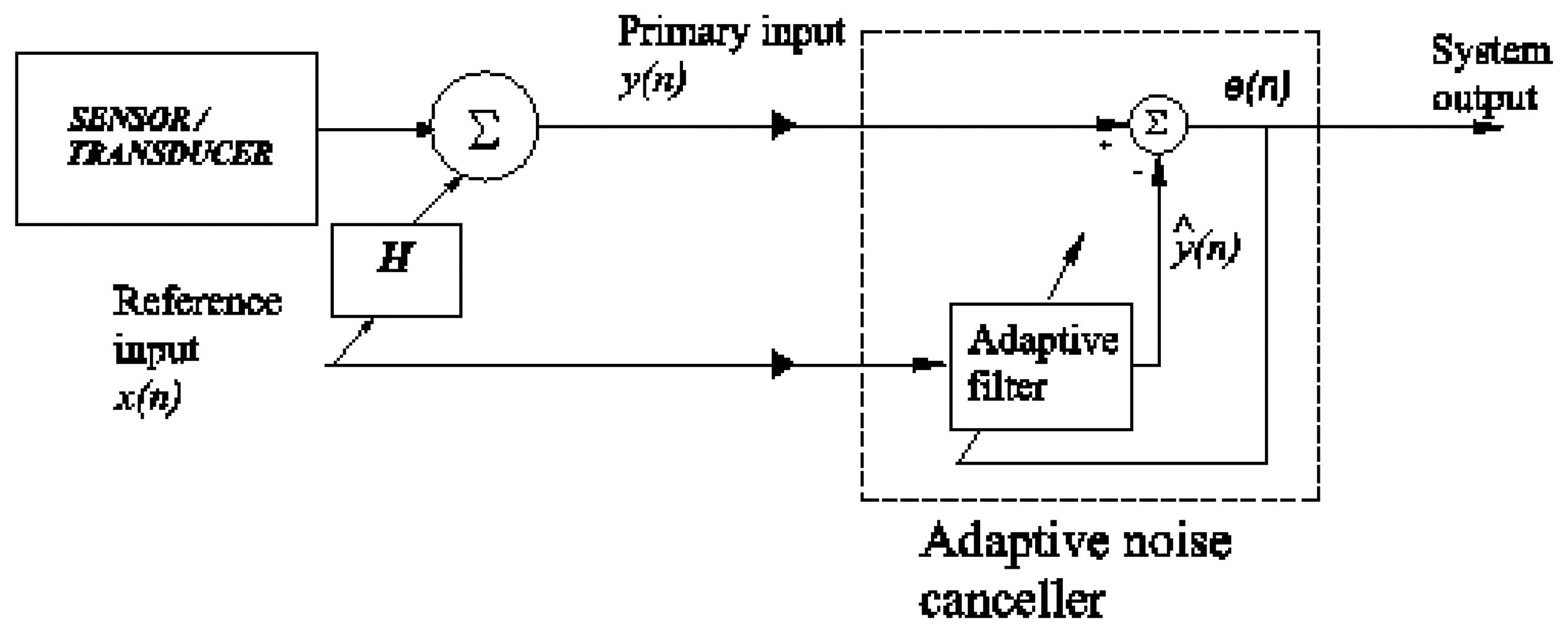
Figure 3.
Primary input (1V = 5kN).

Figure 4.
Normalized mean-squared error of the filter for nine combinations of the length of the filter and the forgetting factor.
Figure 4.
Normalized mean-squared error of the filter for nine combinations of the length of the filter and the forgetting factor.
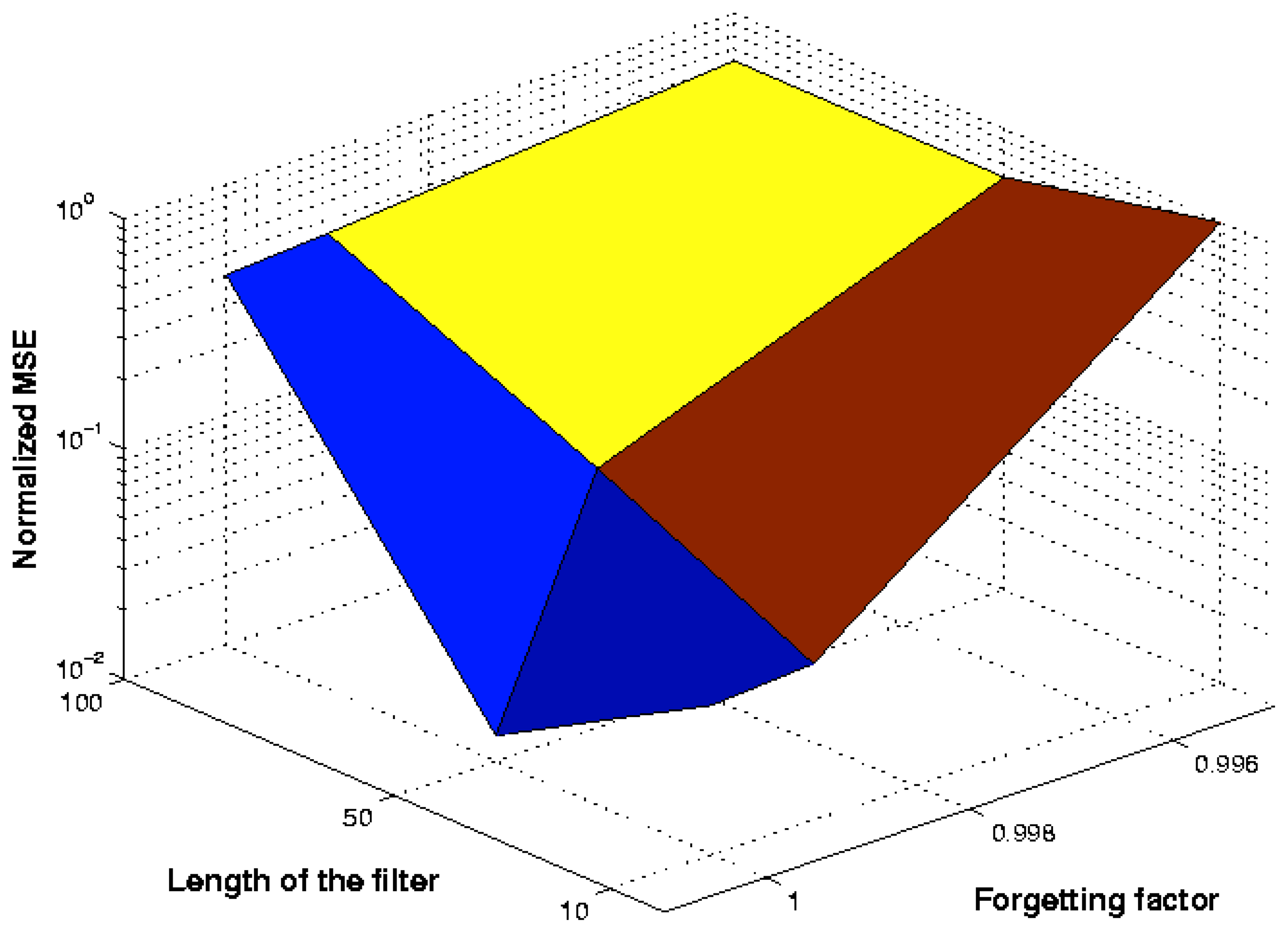
Figure 5.
System output (1V = 5kN).

Figure 6.
Power spectrum magnitude of the primary input and the system output (dB).
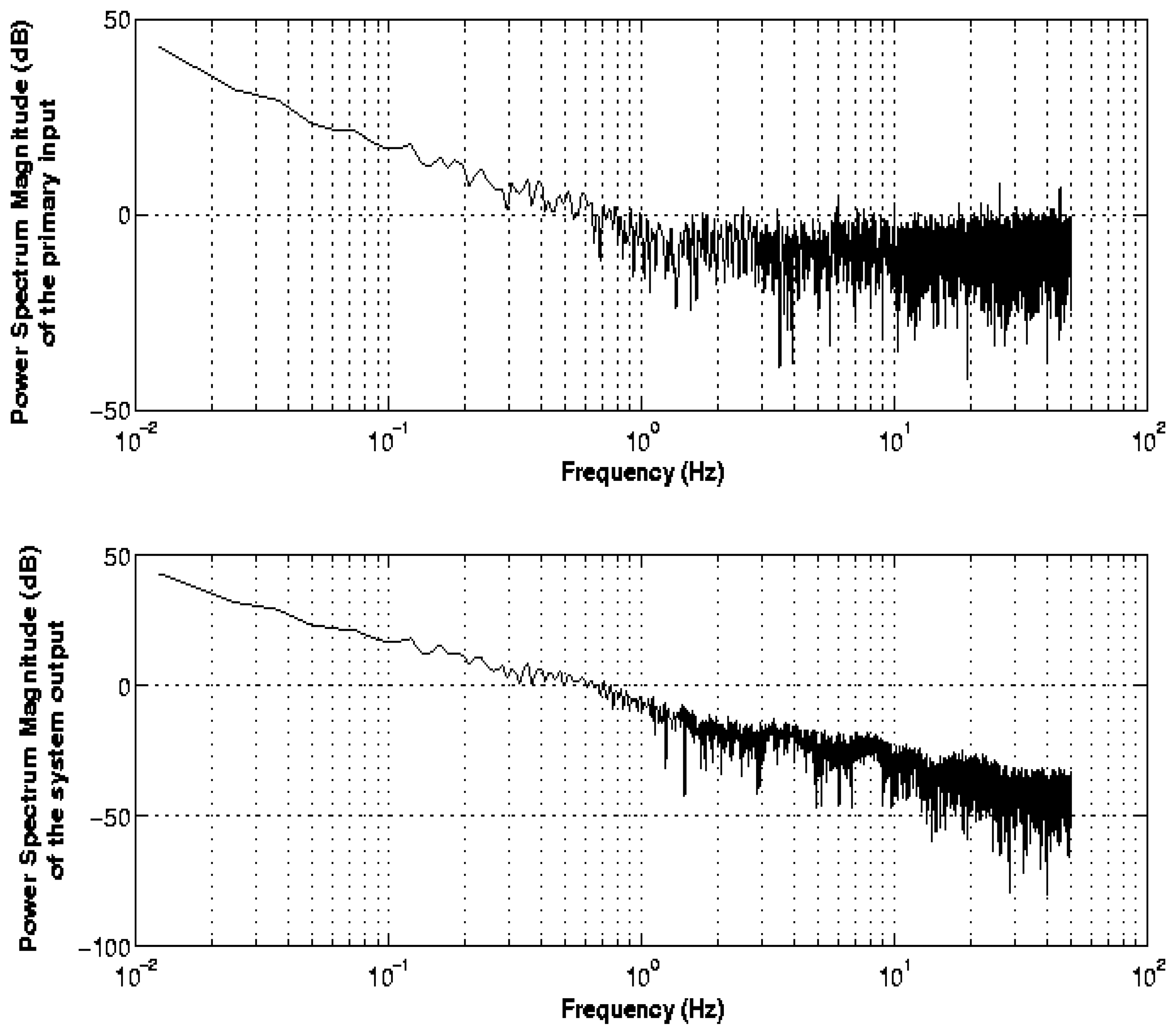
Figure 7.
Learning curve of the RLS lattice adaptive filter
© 2006 by MDPI ( http://www.mdpi.org). Reproduction is permitted for noncommercial purposes.
Share and Cite
MDPI and ACS Style
Hernandez, W. Improving the Response of a Load Cell by Using Optimal Filtering. Sensors 2006, 6, 697-711. https://doi.org/10.3390/s6070697
AMA Style
Hernandez W. Improving the Response of a Load Cell by Using Optimal Filtering. Sensors. 2006; 6(7):697-711. https://doi.org/10.3390/s6070697
Chicago/Turabian StyleHernandez, Wilmar. 2006. "Improving the Response of a Load Cell by Using Optimal Filtering" Sensors 6, no. 7: 697-711. https://doi.org/10.3390/s6070697