Modelling a Peroxidase-based Optical Biosensor

1
Department of Software Engineering, Vilnius University, Naugarduko 24, LT-03225 Vilnius, Lithuania
2
Institute of Mathematics and Informatics, Akademijos 4, LT-08663 Vilnius, Lithuania
3
Department of Chemistry and Bioengineering, Vilnius Gediminas Technical University, Sauletekio al. 11, LT-10223 Vilnius, Lithuania
*
Author to whom correspondence should be addressed.
Sensors 2007, 7(11), 2723-2740; https://doi.org/10.3390/s7112723
Submission received: 8 October 2007
/
Accepted: 9 November 2007
/
Published: 14 November 2007
(This article belongs to the Special Issue Optical Biosensors)
Abstract
:The response of a peroxidase-based optical biosensor was modelled digitally. A mathematical model of the optical biosensor is based on a system of non-linear reaction-diffusion equations. The modelling biosensor comprises two compartments, an enzyme layer and an outer diffusion layer. The digital simulation was carried out using finite difference technique. The influence of the substrate concentration as well as of the thickness of both the enzyme and diffusion layers on the biosensor response was investigated. Calculations showed complex kinetics of the biosensor response, especially at low concentrations of the peroxidase and of the hydrogen peroxide.
1. Introduction
Biosensors are sensors made up of a combination of a biological entity, usually an enzyme, that recognizes a specific analyte and the transducer that translates the biorecognition event into a signal [1, 2]. The signal is proportional to the concentration of the target analyte. The biosensors are classified according to the nature of the physical transducer [3]. Optical biosensors are based on the measurement of absorbed or emitted light resulting from a biochemical reaction [4–6].
Optical biosensors are known to be suitable for environment, clinical and industrial purposes [7]. Those devices allow real-time analysis of molecular interactions without labelling requirements [8]. Optical biosensors have been used to study interactions involving a wide range of interacting partners, from drugs and viruses to peptides, proteins, oligonucleotides, carbohydrates, and lipids [9–13].
The understanding of the kinetic peculiarities of biosensors is of crucial importance for their design. To improve the productivity as well as the efficiency of biosensors design and to optimize the biosensors configuration a model of real biosensors should be build [14, 15]. Starting from seventies various mathematical models of biosensors have been developed and used to study and optimise analytical characteristics of electrochemical biosensors [16–30]. A comprehensive study of the mathematical modelling of amperometric biosensors is given in [31]. Mathematical modelling in the design of optical biosensors has been applied in individual cases only [32, 33].
The goal of this investigation is to make a model allowing an effective computer simulation of peroxidase-based optical biosensors as well as to investigate the influence of the physical and kinetic parameters on the biosensor response. The developed model is based on non-stationary reaction-diffusion equations [34–36]. By changing input parameters the output results were numerically analyzed at transition and steady state conditions.
2. Mathematical Model
We consider the reaction scheme of the optical biosensor involving hydrogen peroxide (H2O2) reaction with peroxidase (E) to form compound I (cmpI) and water (H2O) with the constant reaction rate k1. The compound I interacts with the substrate (S) to form product (P) and free enzyme (E) assuming the constant reaction rate k2,
The product (P) absorbs light and therefore the response of the biosensor increases during the reaction as the product forms. The concentration of the analyte (S) can be directly determined from the absorbance of the product (P) [37].
Assuming the symmetrical geometry of the biosensor and homogeneous distribution of immobilized enzyme, the mass transport and the reaction kinetics in the enzyme layer can be described by the following system of the reaction-diffusion equations (0 < x < d, t > 0),
where x and t stand for space and time, Se(x, t), Pe(x, t), He(x, t), E(x, t), C(x, t); are the substrate, product, hydrogen peroxide, peroxidase and compound I concentrations in the enzyme layer, d is the thickness of the enzyme layer, and Dse, Dpe, DHe are the diffusion coefficients. The enzyme and the formed compound I are immobilized and therefore there are no diffusion terms in the enzyme and compound I equations.
Outside the enzyme layer only mass transport by diffusion of the substrate, product and hydrogen peroxide takes place. We assume that the external mass transport obeys a finite diffusion regime (d < x < d + δ, t > 0),
where δ is the thickness of the diffusion layer, Sb(x, t), Pb(x, t), Hb(x, t) are the substrate, product and hydrogen peroxide concentrations in the diffusion layer, and DSb, DPb, DHb are the diffusion coefficients.
The diffusion layer (d < x < d + δ) may be treated as the Nernst diffusion layer [38]. According to the Nernst approach a layer of thickness δ remains unchanged with time. It was assumed that away from it the solution is uniform in concentration.
Let x = 0 represents the plate surface, while x = d is the boundary between the enzyme layer and the buffer solution. The biosensor operation starts when some substrate appears in the bulk solution. This is used in the initial conditions (t = 0)
where E0 stands for the initial concentration of the enzyme in the enzyme layer, H0 is the hydrogen peroxide concentration in the bulk solution as well as in the enzyme layer, and S0 is the substrate concentration in the bulk solution.
In the bulk solution the concentrations of the substrate, product and hydrogen peroxide remain constant (t > 0),
Assuming the impenetrable and unreactive plate surface, the mass flux of the species must vanish at this boundary,
On the boundary between two regions having different diffusivities, we define the matching conditions (t > 0)
These conditions mean that fluxes of the substrate, product and hydrogen peroxide through the stagnant external diffusion layer equals to the corresponding fluxes entering the surface of the enzyme layer. The partitions of the substrate, product and hydrogen peroxide in the enzyme layer versus bulk are assumed to be equal [24, 28].
The light absorbance was assumed as the response of the optical biosensor. The optical signal is due to the product absorbance in the enzyme and diffusion layers. The optical biosensor was assumed to be placed in the flow or inside of a very high volume of mixed solution. The product molecules which escape the enzyme and diffusion layers do not contribute to the signal. The absorbance A(t) at time t may be obtained as follows:
where εP is molar extinction coefficient of the product, (P̄) - the concentration of the product averaged through the enzyme and diffusion layers, lef - the effective thickness of the enzyme layer and Nernst layer [37]. For organic compounds εP varies between 104 and 102 m2mol−1.
For the further representation of averaged concentrations of substrate, product and hydrogen peroxide through the enzyme and diffusion layers, we introduce the following designations:
The concentrations of the substrate, product, hydrogen peroxide, enzyme and compound I averaged only through the enzyme layer are given by
We assume that the system (3), (4), (5), (6), (7), (8), (9), (10), (11), (12), (13) and (14) approaches a steady state as t →∞,
where A∞ is the steady state absorbance.
The reaction product may be fluorescent and it may be the fluorescence which is measured [4, 6]. The fluorescence can be expressed as an inversely exponential function of the average concetration of the product [37]. Since the optical absorbance is directly propotional to the concentration of the reaction product (see (15)), the fluorescence can be calculated from the corresponding absorbance. Because of this, the dynamics of only species concentrations and of the absorbance is analysed below.
The sensitivity is another very important characteristic of biosensors [1, 2]. It is defined as a gradient of the steady state absorbance with respect to the substrate concentration. The absorbance varies in orders of magnitude with the concentration of the substrate to be analyzed [4]. Therefore dimensionless expression of the sensitivity is preferable,
where BS stands for the dimensionless sensitivity of the biosensor, A∞(S0) is the steady state absorbance calculated at the substrate concentration S0 in bulk solution.
We consider the dimensionless Biot number Bi to express the ratio of internal mass transfer resistance to the external one [34],
3. Digital Simulation
Because of non-linearity of the problem, no analytical solutions are possible [34, 39]. Hence numerical simulation is employed. We applied a uniform discrete grid to simulate the biosensor using implicit finite difference method [24, 27, 40]. The program was implemented in Java programming language [41].
We assume the biosensor response AR calculated at the moment TR as the steady state response,
where τ stands for the size of time step. We used ε = 10−3 for the calculations. The response time TR as an approximate steady state time is highly sensitive to the decay rate ε, i.e. TR →∞ when ε → 0. We introduce less sensitive part of the steady state time function A*(t)
T0.5 is defined as the time at which a half of the steady state absorbance is reached, i.e., A*(T0.5) = 0.5. T0.5 is usually called the half time of the steady state.
The following values of the model parameters were employed in all the numerical experiments:
The following constant-concentration conditions can be derived from equations (3), (4), (5), (6), (7), (8), (9), (10), (11), (12), (13) and (14):
These conditions were employed in testing the numerical solution of the model.
4. Results and Discussion
By changing input parameters the output results were numerically analyzed with special emphasis to the influence of the biosensor geometry and of the catalytical parameters on the biosensor response at transition and steady state conditions.
4.1. The Dynamics of the Concentrations of the Compounds
Figs. 1 and 2 show the concentration profiles of substrate, product, hydrogen peroxide, compound I and enzyme peroxidase in the enzyme and diffusion layers. These concentration profiles were obtained when the steady state and the half of it was reached.
As one can see in Figs. 1 and 2, constraints (26) on the concentrations are ensured. When the biosensor operation starts, the initial (t = 0) concentration of the enzyme (E) equals E0 and the compound I (C) starts at zero concentration. Fig. 1 shows, that the final (at steady state conditions) concentration E of the enzyme is less than 0.3% of the initial concentration E0 while the concentration C of the compound I is equal approximately to the initial concentration E0 of the enzyme. These concentrations quickly become invariable. The dynamics of the substrate concentration is also quit fast. The final (steady state) concentrations of these three compounds differ only slightly from the concentrations obtained at the half time of the steady state. The concentrations of the hydrogen peroxide (He, Hb) and of the product (Pe, Pb) change notably slower.
Although the dependence of the product concentration is linear as seen in Fig. 2, the linear dependence is not followed in the enzyme layer (1 μm). This is highlighted in the inset of Fig. 2. The non-linear dependence could be explained by the enzymatic reaction occurring in the enzyme layer.
The dynamics of the concentrations of the compounds is also presented in Figs. 3 and 4. Fig. 3 shows the concentrations averaged through the enzyme layer while Fig. 4 shows the concentrations averaged through both compartments, the enzyme layer and the diffusion layer. The thickness d of the enzyme layer equals 1 μm. The thickness δ of the external diffusion layer is in two orders of magnitude higher, δ = 400μm = 400d . After a certain time the equilibrium approaches and the concentrations become invariable.
During the biosensor action the substrate diffuses into the enzyme layer and this results in a decrease of the enzyme as well as of the hydrogen peroxide and in an increase of the compound I as well as of the product concentrations. The inset in Fig. 3 shows very high concentration dynamics of the enzyme (Ē) as well as of the compound I (C̄) in the beginning of the reacting process. In about 1 ms these concentrations become approximately constant. The concentration dynamics of all other compounds is significantly lower.
Figs. 5 and 6 present the averaged concentrations for tenfold thinner enzyme layer (d = 0.1μm). One can observe similar concentration evolution as in the previous case, with some differences from a quantitative point of view. The shortage of compound I results to larger amounts of unreacted hydrogen peroxide and substrate.
Fig. 5 also shows non-monotony of Ē and C̄ as functions of time t. The inset in Fig. 5 shows very fast reduction of the enzyme (Ē) and so fast growth of the compound I (C̄). In about 0.5 ms practically whole enzyme peroxidase converts to compound I. In about 10 s some substrate reaches the enzyme layer and the reaction (2) starts. Because of this, the enzyme (Ē) is regenerated from the compound I (C̄). Fig. 5 expressly shows that biosensor action starts very quickly with the reaction (1) while the reaction (2) starts with notable delay. Certainly, the delay term depends on the thickness δ of the external diffusion layer.
4.2. The Impact of the Thickness of the Diffusion Layer
The dependence of the absorbance on the thickness of the diffusion layer is shown in the Fig. 7. The Biot number Bi was calculated assuming a constant thickness of the enzyme layer. The absorbance increases with an increase in the substrate concentration. The absorbance strongly depends on the outer concentration S0 of the substrate whereas the effect of other parameters is notably less important. In cases of a thick diffusion layer (Bi <≈ 0.02 or δ >≈ 100μm) only the substrate concentration effects the absorbance. The concentration of the product (which absorbs light) directly depends on the concentration of the substrate, thus the absorbance changes in relation to the concentration of the substrate.
The approximately linear decrease of the steady state absorbance AR with the Biot number Bi can be explained by a linear distancing the border (x = d + δ) where the product concentration is permanently reduced to zero (see the boundary condition (12)). Consequently, the exact evaluation of the thickness of the external (Nernst) diffusion layer is of crucial importance to predict the biosensor response accurately.
As one can see in Fig. 7, the gradient of the steady state absorbance AR as a function of the Biot number Bi is notably lower at lower initial concentrations of the enzyme (E0, curve 5) as well as of the hydrogen peroxide (H0, curve 7) rather than at higher ones (corresponding curves 4 and 6). Thus, the absorbance is less sensitive to changes in the thickness δ of the external diffusion layer (which is reversally proportional to the Biot number Bi) at higher values of E0 and H0 than at lower ones.
The response time increases with thickening the diffusion layer due to the time delay needed for substrate to appear in the enzyme layer (Fig. 8). A tenfold increase in the thickness δ increases the response time approximately hundredfold. All other considered parameters affect the biosensor response time slightly. The half time T0.5 of the steady state response is approximately a linear function of the Biot number Bi as well as of the thickness δ of the diffusion layer. Slight variations in the linear behaviour of T0.5 can be explained by a non-linearity of the reaction process in the enzyme layer (see the inset in Fig. 2).
Observed values of the biosensor sensitivity are fairly high except two cases (see Fig. 9). At high outer substrate concentration S0 the enzyme becomes saturated and cannot respond effectively to the change of the substrate concentration (see curve 2). Very similar results were obtained at low concentration H0 of the hydrogen peroxide (curve 7). The decrease in the initial enzyme concentration E0 (curve 5) also determines a decrease in the sensitivity of the biosensor response. However, in all the cases increase in the thickness of the diffusion layer (i.e. decrease of the Biot number) positively effects the biosensor sensitivity.
A relatively short linear range of the calibration curve is one of serious drawbacks restricting wider use of the biosensor [1, 2, 7]. This problem can be partially solved by an application of an additional inert outer membrane on the surface of the enzyme layer [1, 2, 7]. In the case of optical biosensors, outer membranes are of limited applicability [5, 6]. Therefore, an opportunity to increase the biosensor sensitivity as well as the linear range of the calibration curve by increasing the thickness of the external diffusion layer is especially important.
4.3. The Impact of the Thickness of the Enzyme Layer
The effect of enzyme layer thickness on the absorption, response time and sensitivity was analyzed. In this test problem the Biot number was calculated assuming a constant thickness of the diffusion layer.
In general, the importance of the enzyme layer (membrane) thickness to the biosensor response is rather well known [1, 2, 15, 17, 21, 22, 30]. Usually, the effect of the enzyme layer thickness decreases with an increase in the layer thickness. Fig. 10 shows that in the case of the peroxidase-based optical biosensor, the enzyme layer thickness d effects the absorbance AR slightly only. This can be explained by relatively thick external diffusion layer [21, 22]. The analyzed thickness δ of the external diffusion layer was in several orders of magnitude greater than the enzyme layer thickness d. The biosensor response is highly stable to changes in the enzyme layer thickness when the Biot number Bi varies from 0.02 to 0.2 (the thickness d varies from 0.01δ up to 0.1δ). The high stability of the biosensor response to changes in the enzyme layer thickness is a useful characteristic for the biosensor developers [5, 6].
In addition, Fig. 10 shows that the absorbance strongly depends on the bulk concentration S0 of the substrate. Below this property is discussed in detail.
Fig. 11 shows the effect of the Biot number, which is directly proportional to the enzyme layer thickness d, on the half time T0.5 of the steady state response of the optical biosensor. In most cases the half time T0.5 is a non-monotonous function of the thickness d. This is especially notable in the case of low concentration of enzyme compared to the concentrations of substrate and hydrogen peroxide (curve 5). The behaviour of the half time T0.5 when changing the enzyme layer thickness d at high substrate concentration S0 as compared to the concentrations of enzyme and hydrogen peroxide (curve 2) is very similar to that at low (see the parameters in Fig. 7) concentration H0 of the hydrogen peroxide (curve 7). Only in both these cases (curves 2 and 7) the half time T0.5 is a monotonous function of d. However, in all the cases when the enzyme layer is relatively thick (Bi >≈ 0.2 or d >≈ 10 μm) T0.5 is a monotonous increasing function of d at all values of the parameters.
The effect of the Biot number Bi on the biosensor sensitivity BS is depicted Fig. 12. The effect of the layer thickness is rather similar to that of the external diffusion layer. The sensitivity of the biosensor increases extending the enzyme layer (Fig. 12). The observed values of the sensitivity are very high except two cases (curves 2 and 7). The sensitivity is notable lower at a high concentration S0 of the substrate (curve 2) and at a low concentration H0 of the hydrogen peroxide (curve 7) as compared to the values of other concentrations. In both these cases the biosensor sensitivity BS is rather sensitive to changes in the enzyme layer thickness d. At a high concentration S0 as well as at a low concentration H0 (see the parameters in Fig. 7) the biosensor sensitivity BS can be notably increased by increasing the thickness d of the enzyme layer.
4.4. The Impact of the Outer Substrate Concentration
In this test problem the outer substrate concentration is expressed as the ratio of the substrate and hydrogen peroxide concentrations combining with the rates of the corresponding reactions (1) and (2)
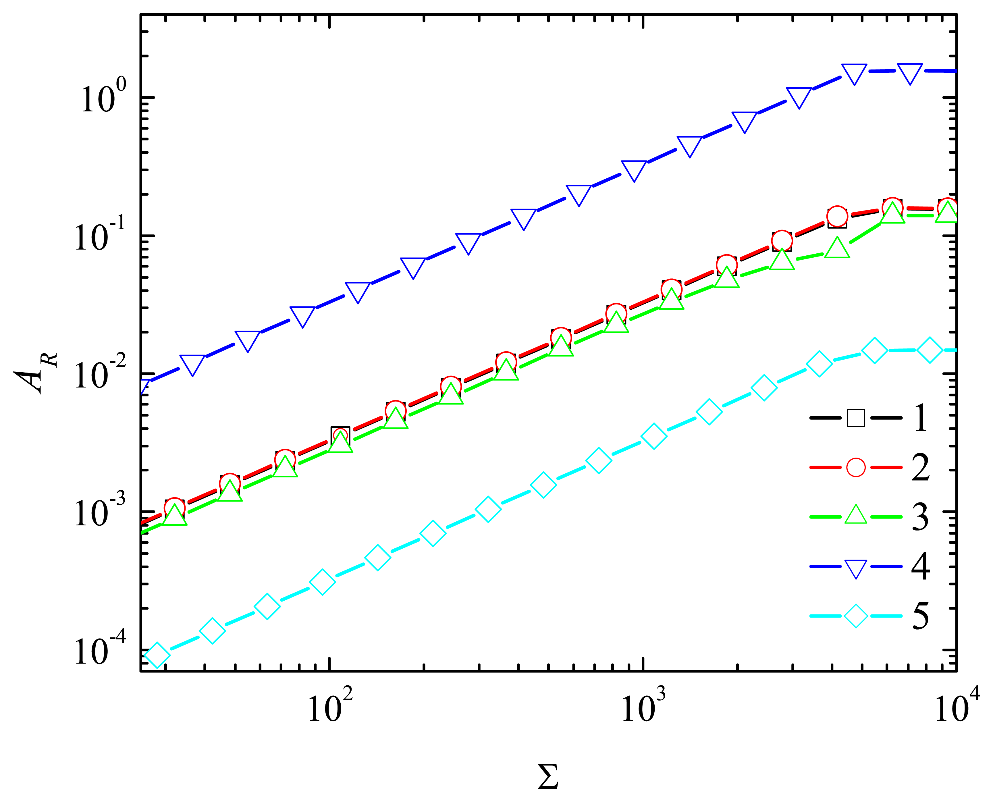
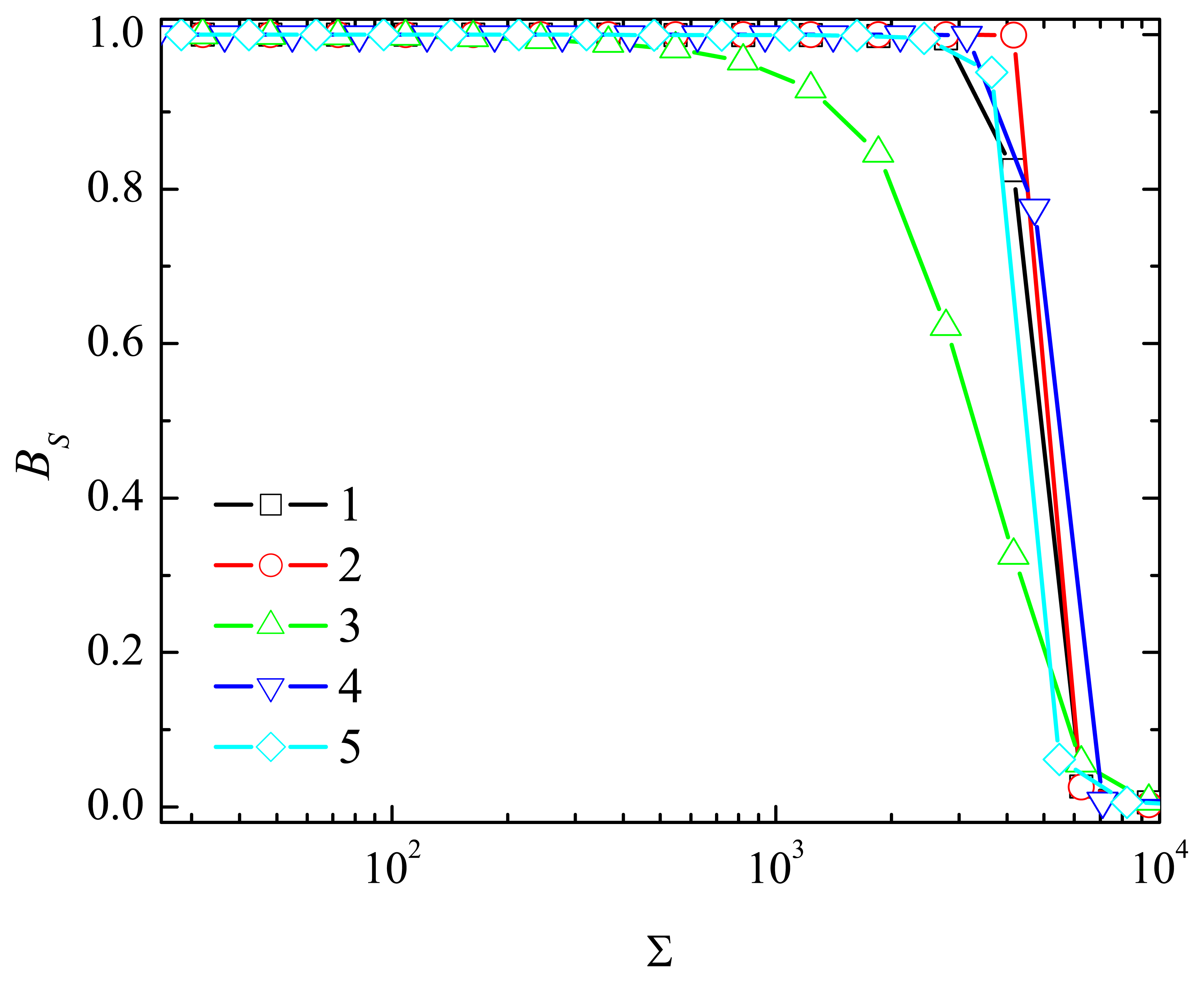
The dependence of the absorbance and sensitivity of the biosensor on the dimensionless ratio Σ of the reactions (2) and (1) is depicted in the Figs. 13 and 14, respectively.
One can see in Fig. 13 a linear range of the calibration curve up to Σ ≈ 5 × 10³ (S0 ≈ 200 μM). The dependence of the absorbance AR on the ratio Σ is noticeably affected by the hydrogen peroxide (H0). The absorbance is directly proportional to the concentration H0 of the hydrogen peroxide. A tenfold increase in the concentration H0 increases the absorbance approximately tenfold (curve 4). The corresponding decrease in H0 decreases the AR tenfold (curve 5). A variation in the initial concentration E0 of enzyme effects the absorbance slightly (curves 2 and 3).
Fig. 14 shows, that the biosensor sensitivity notably decreases with a decrease in the concentrations E0 on the enzyme (curve 3). The concentrations of the enzyme and of the hydrogen peroxide determine the concentration of the compound I (reaction (1)), which interacts with the substrate to form the product (reaction (2)). A decrease in enzyme concentration E0 decreases the rate of product formation, while an increase in substrate concentration S0 increases the reaction rate up to saturation [1, 2]. A lower concentration E0 of the enzyme corresponds to a lower substrate concentration S0 at which the enzyme is saturated with the substrate. Fig. 14 show this effect as a decreasing sensitivity of the biosensor with a decrease in the enzyme concentration E0.
5. Conclusions
The mathematical model (3), (4), (5), (6), (7), (8), (9), (10), (11), (12), (13) and (14) of a peroxidase-based optical biosensor can be successfully used to investigate the kinetic peculiarities of the biosensor response.
The sensitivity of the optical biosensor increases with an increase in the thickness δ of the external diffusion layer (Fig. 9). The light absorbance is less sensitive to changes in the thickness δ at higher concentrations of the enzyme and of the hydrogen peroxide than at lower concentrations of those species.
Assuming the relatively thick external diffusion layer, the biosensor response is highly stabile to changes in the enzyme layer thickness d when d varies from one hundredth to one tenth of the thickness δ of the diffusion layer (0.01δ < d < 0.1δ, Fig. 10). The response stability to changes in d reduces at low concentrations of the hydrogen peroxide and at high concentrations of the substrate (Fig. 12).
The sensitivity of the optical biosensor decreases with a decrease in the concentration of the enzyme (Fig. 14).
To prove conclusions made the experiments are running using peroxidase-based optical biosensors with different geometry and catalytical parameters.
Acknowledgments
The authors express sincere gratitude to prof. Feliksas Ivanauskas for his valuable contribution into modelling of biosensors.
References
- Scheller, F.; Schubert, F. Biosensors; Elsevier: Amsterdam, 1992. [Google Scholar]
- Turner, A. P. F.; Karube, I.; Wilson, G. S. Biosensors: Fundamentals and Applications; Oxford University Press: Oxford, 1987. [Google Scholar]
- Chaubey, A.; Malhotra, B. D. Mediated biosensors. Biosens. Bioelectron. 2002, 17(6), 441–456. [Google Scholar]
- Ligler, F. S.; Taitt, C. R. Optical Biosensors: Present and Future; Elsevier Science: Amsterdam, 2002. [Google Scholar]
- Choi, M. M. F. Progress in enzyme-based biosensors using optical transducers. Microchimica Acta 2004, 148(3-4), 107–132. [Google Scholar]
- Bosch, M. E.; Sánchez, A. J. R.; Rojas, F. S.; Ojeda, C. B. Recent development in optical fiber biosensors. Sensors 2007, 7(6), 797–859. [Google Scholar]
- Wollenberger, U.; Lisdat, F.; Scheller, F. W. Frontiers in Biosensorics 2. Practical Applications; Birkhauser Verlag: Basel, 1997. [Google Scholar]
- Leatherbarrow, R. J.; Edwards, P. R. Analysis of molecular recognition using optical biosensors. Curr. Opin. Chem. Biol. 1999, 3(5), 544–547. [Google Scholar]
- Ojeda, C. B.; Rojas, F. S. Recent development in optical chemical sensors coupling with flow injection analysis. Sensors 2006, 6(10), 1245–1307. [Google Scholar]
- Wu, B.; Wang, Y.; Li, J.; Song, Z.; Huang, J.; Wang, X.; Chen, Q. An optical biosensor for kinetic analysis of soluble interleukin-1 receptor i binding to immobilized interleukin-1α. Talanta 2006, 70(3), 485–488. [Google Scholar]
- Stefano, L. D.; Arcari, P.; Lamberti, A.; Sanges, C.; Rotiroti, L.; Rea, I.; Rendina, I. DNA optical detection based on porous silicon technology: from biosensors to biochips. Sensors 2007, 7(2), 214–221. [Google Scholar]
- Passaro, V. M. N.; Dell’olio, F.; Casamassima, B.; Leonardis, F. D. Guided-wave optical biosensors. Sensors 2007, 7(4), 508–536. [Google Scholar]
- Sanz, V.; de Marcos, S.; Galbán, J. Direct glucose determination in blood using a reagentless optical biosensor. Biosens. Bioelectron. 2007, 22(12), 2876–2883. [Google Scholar]
- Ferreira, L. S.; Souza, M. B. D.; Trierweiler, J. O.; Broxtermann, O.; Folly, R. O. M.; Hitzmann, B. Aspects concerning the use of biosensors for process control: experimental and simulation investigations. Comp. Chem. Engng. 2003, 27(8), 1165–1173. [Google Scholar]
- Corcuera, J. R. D.; Cavalieri, R.; Powers, J.; Tang, J. Amperometric enzyme biosensor optimization using mathematical modeling. Proceedings of the 2004 ASAE / Csae Annual International Meeting, page Paper No. 047030. Ottawa, Ontario, Canada, (August 1-4 2004); American Society of Agricultural Engineers.
- Mell, C.; Maloy, J. T. A model for the amperometric enzyme electrode obtained through digital simulation and applied to the glucose oxidase system. Anal. Chem. 1975, 47, 299–307. [Google Scholar]
- Kulys, J. The development of new analytical systems based on biocatalysts. Anal. Lett. 1981, 14, 377–397. [Google Scholar]
- Bartlett, P. N.; Pratt, K. F. E. Modelling of processes in enzyme electrodes. Biosens. Bioelectron. 1993, 8(9-10), 451–462. [Google Scholar]
- Schulmeister, T.; Pfeiffer, D. Mathematical modelling of amperometric enzyme electrodes with perforated membranes. Biosens. Bioelectron. 1993, 8(2), 75–79. [Google Scholar]
- Yokoyama, K.; Kayanuma, Y. Cyclic voltammetric simulation for electrochemically mediated enzyme reaction and determination of enzyme kinetic constants. Anal. Chem. 1998, 70(16), 3368–3376. [Google Scholar]
- Lyons, M. E. G.; Murphy, J.; Rebouillat, S. Theoretical analysis of time dependent diffusion, reaction and electromigration in membranes. J. Solid State Electrochem. 2000, 4, 458–472. [Google Scholar]
- Baronas, R.; Ivanauskas, F.; Kulys, J. The influence of enzyme membrane thickness on the response of amperometric biosensors. Sensors 2003, 3(7), 248–262. [Google Scholar]
- Baronas, R.; Kulys, J.; Ivanauskas, F. Modelling amperometric enzyme electrode with substrate cyclic conversion. Biosens. Bioelectron. 2004, 19(8), 915–922. [Google Scholar]
- Baronas, R.; Ivanauskas, F.; Kulys, J. Computer simulation of the respose of amperometric biosensors in stirred and non stirred solution. Nonlinear Anal. Model. Control 2003, 8(1), 3–18. [Google Scholar]
- Baronas, R.; Kulys, J.; Ivanauskas, F. Mathematical model of the biosensors acting in a trigger mode. Sensors 2004, 4(4), 20–36. [Google Scholar]
- Lyons, M. E. G. Modelling the transport and kinetics of electroenzymes at the electrode/solution interface. Sensors 2006, 6(12), 1765–1790. [Google Scholar]
- Baronas, R.; Kulys, J.; Ivanauskas, F. Computational modelling of biosensors with perforated and selective membranes. J. Math. Chem. 2006, 39(2), 345–362. [Google Scholar]
- Kulys, J.; Baronas, R. Modelling of amperometric biosensors in the case of substrate inhibition. Sensors 2006, 6(11), 1513–1522. [Google Scholar]
- Popovtzer, R.; Natan, A.; Shacham-Diamand, Y. Mathematical model of whole cell based bio-chip: an electrochemical biosensor for water toxicity detection. J. Electroanal. Chem. 2007, 602(1), 17–23. [Google Scholar]
- Baronas, R.; Ivanauskas, F.; Kulys, J. Computational modelling of the behaviour of potentiometric membrane biosensors. J. Math. Chem. 2007, 42(3), 321–336. [Google Scholar]
- Schulmeister, T. Mathematical modelling of the dynamic behaviour of amperometric enzyme electrodes. Selective Electrode Rev. 1990, 12, 203–260. [Google Scholar]
- Merino, S.; Grinfeld, M.; McKee, S. A degenerate reaction diffusion system modelling an optical biosensor. Z. angew. Math. Phys. 1998, 49(1), 46–85. [Google Scholar]
- Rickus, J. L. Impact of coenzyme regeneration on the performance of an enzyme based optical biosensor: a computational study. Biosens. Bioelectron. 2005, 21(6), 965–972. [Google Scholar]
- Aris, R. The Mathematical Theory of Diffusion and Reaction in Permeable Catalysts. The Theory of the Steady State; Clarendon Press: Oxford, 1975. [Google Scholar]
- Carr, P. W.; Bower, L. D. Immobilized Enzymes in Analytical and Clinical Chemistry: Fundamentals and Applications; John Wiley: New York, 1980. [Google Scholar]
- Kernevez, J. P. Enzyme Mathematics. Studies in Mathematics and its Applications; Elsevier Science: Amsterdam, 1980. [Google Scholar]
- Vo-Dinh, T. Biomedical Photonics Handbook; CRC Press LLC: New York, 2003. [Google Scholar]
- Wang, J. Analytical Electrochemistry, 2nd Ed. ed; Springer-Verlag: Berlin, 1988. [Google Scholar]
- Britz, D. Digital Simulation in Electrochemistry, 3rd Ed. ed; Springer-Verlag: Berlin, 2005. [Google Scholar]
- Samarskii, A. A. The Theory of Difference Schemes; Marcel Dekker: New York-Basel, 2001. [Google Scholar]
- Moreira, J. E.; Midkiff, S. P.; Gupta, M.; Artigas, P. V.; Snir, M.; Lawrence, R. D. Java programming for high-performance numerical computing. IBM Systems Journal 2000, 39(6), 21–56. [Google Scholar]
Figure 1.
The steady state (TR = 305 s, 1) and the half of it (T0.5 = 116 s, 2) concentration profiles of compound I (C) and peroxidase (E) in the enzyme layer (d = 1μm) at S0 = 100μM, E0= 1 nM, H0 = 1 mM, δ = 400 μm.
Figure 1.
The steady state (TR = 305 s, 1) and the half of it (T0.5 = 116 s, 2) concentration profiles of compound I (C) and peroxidase (E) in the enzyme layer (d = 1μm) at S0 = 100μM, E0= 1 nM, H0 = 1 mM, δ = 400 μm.
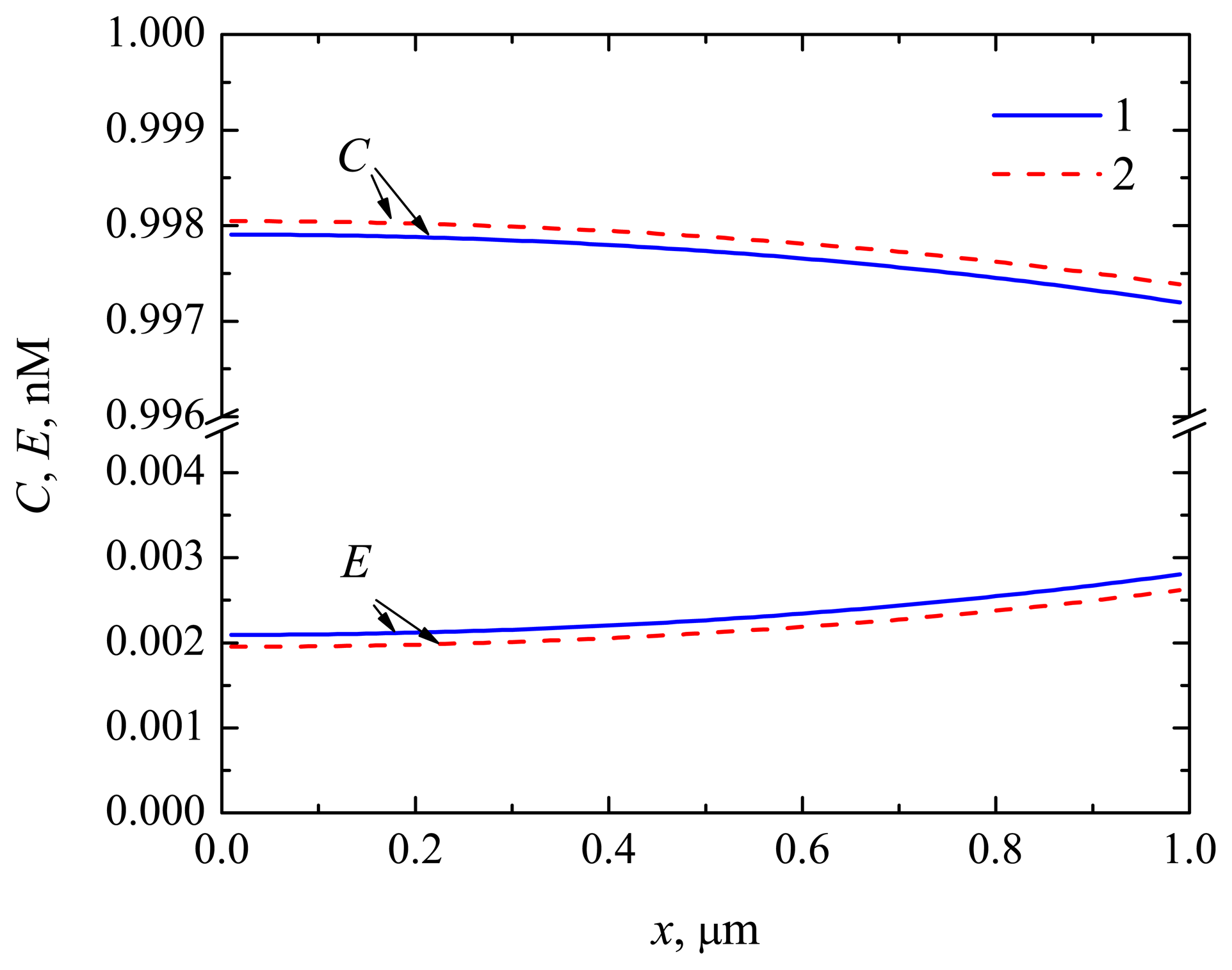
Figure 2.
The concentration profiles of the substrate (Se,b), product (Pe,b) and hydrogen peroxide (He,b) in the enzyme layer and diffusion layers. The parameters and notation are the same as in Fig. 1.
Figure 2.
The concentration profiles of the substrate (Se,b), product (Pe,b) and hydrogen peroxide (He,b) in the enzyme layer and diffusion layers. The parameters and notation are the same as in Fig. 1.
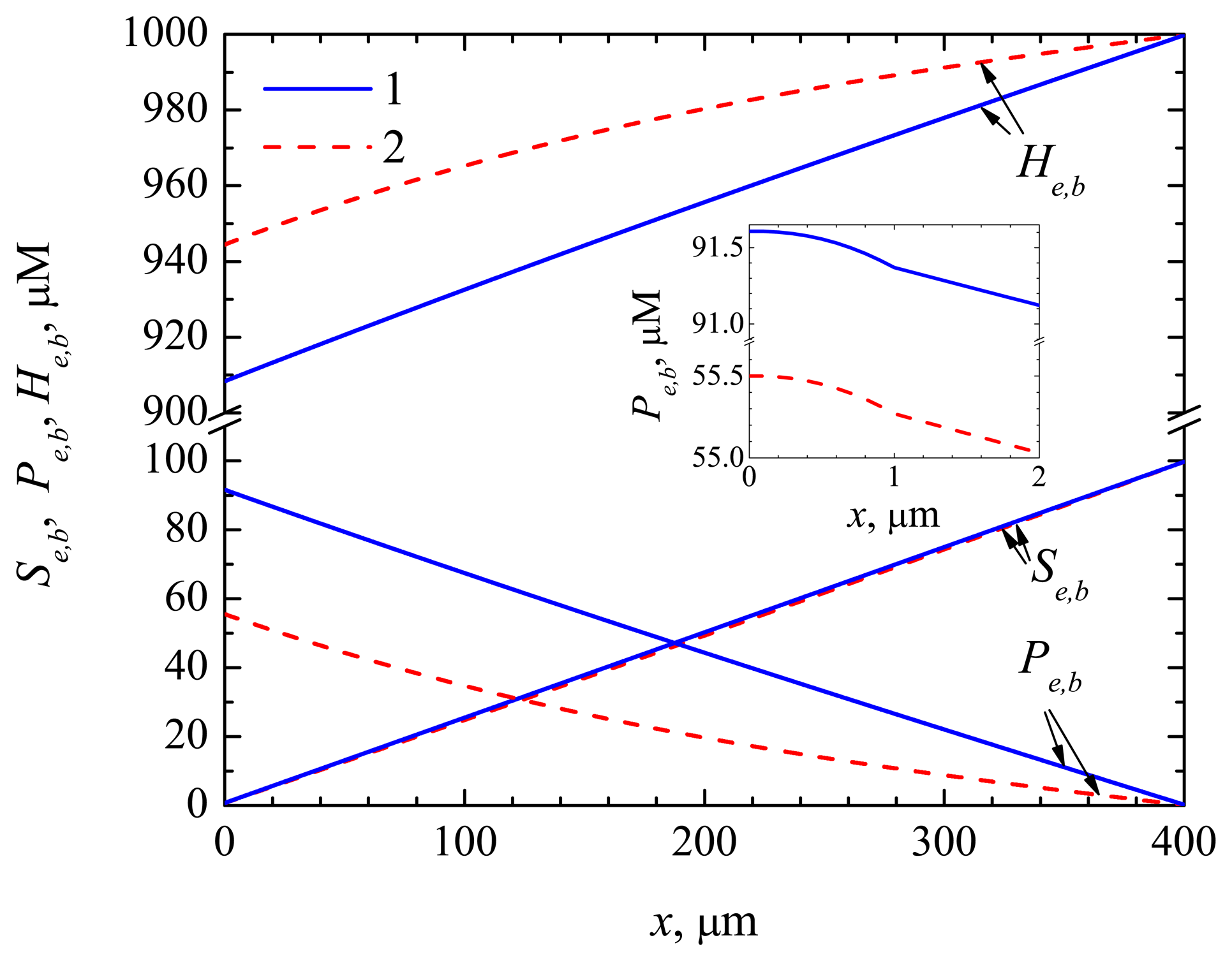
Figure 3.
The concentrations of the substrate (S̄e), product (P̄e), hydrogen peroxide (H̄e), compound I (C̄) and enzyme (Ē) averaged through the enzyme layer (d = 1μm). The parameters are the same as in Fig. 1.
Figure 3.
The concentrations of the substrate (S̄e), product (P̄e), hydrogen peroxide (H̄e), compound I (C̄) and enzyme (Ē) averaged through the enzyme layer (d = 1μm). The parameters are the same as in Fig. 1.
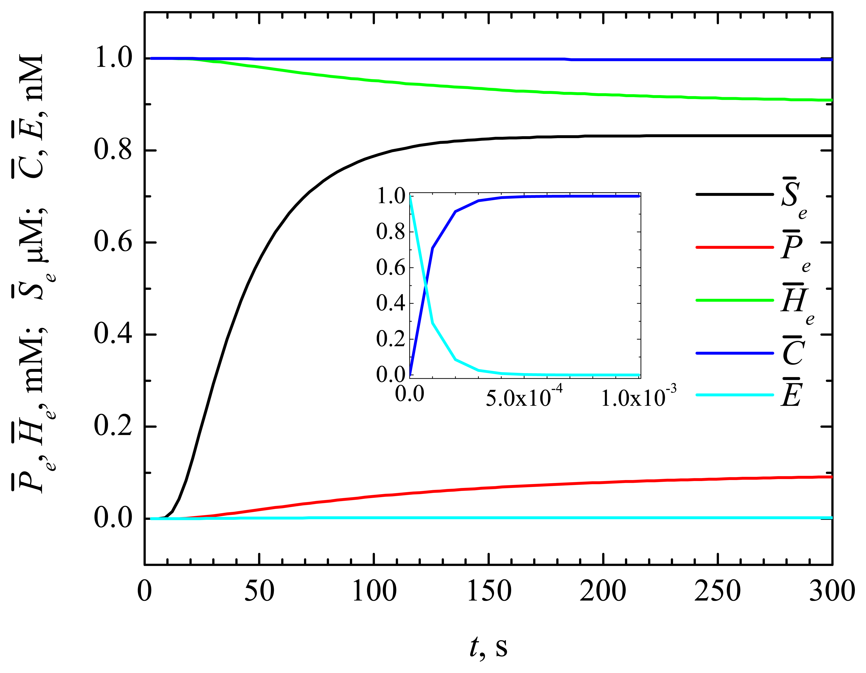
Figure 4.
The concentrations of the substrate (S̄), product (P̄) and hydrogen peroxide (H̄) averaged through the enzyme and diffusion layers. The parameters are the same as in Fig. 1.
Figure 4.
The concentrations of the substrate (S̄), product (P̄) and hydrogen peroxide (H̄) averaged through the enzyme and diffusion layers. The parameters are the same as in Fig. 1.
Figure 5.
The concentrations of substrate (S̄e), product (P̄e), hydrogen peroxide (H̄e), compound I (C̄) and enzyme (Ē) averaged through the enzyme layer of the thickness d = 0.1μm. Other parameters are the same as in Fig. 1.
Figure 5.
The concentrations of substrate (S̄e), product (P̄e), hydrogen peroxide (H̄e), compound I (C̄) and enzyme (Ē) averaged through the enzyme layer of the thickness d = 0.1μm. Other parameters are the same as in Fig. 1.
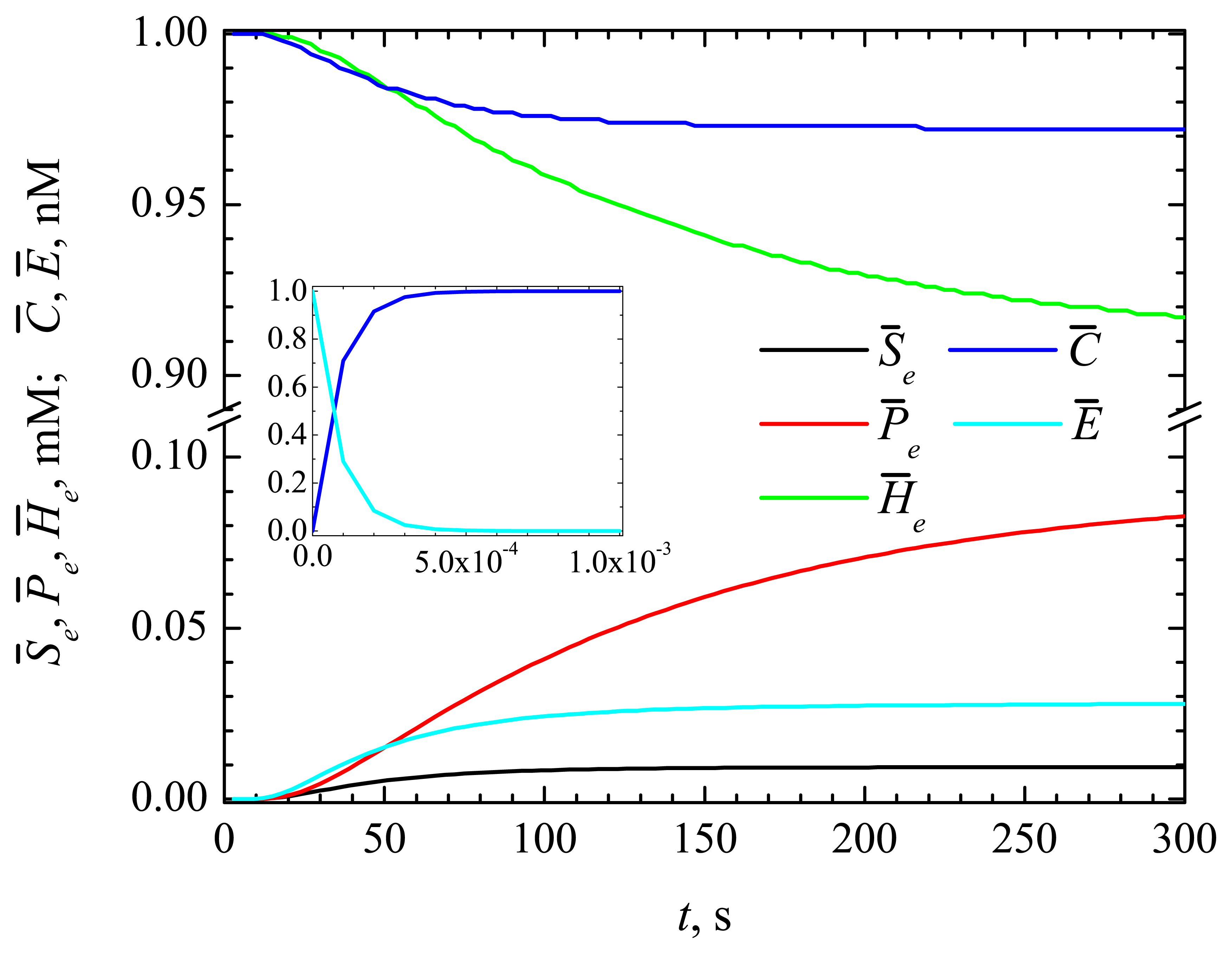
Figure 6.
The concentrations of substrate (S̄), product (P̄) and hydrogen peroxide (H̄) averaged through the enzyme and diffusion layers at the thickness d = 0.1μm of the enzyme layer. Other parameters are the same as in Fig. 1.
Figure 6.
The concentrations of substrate (S̄), product (P̄) and hydrogen peroxide (H̄) averaged through the enzyme and diffusion layers at the thickness d = 0.1μm of the enzyme layer. Other parameters are the same as in Fig. 1.

Figure 7.
Dependence of the absorbance AR on the Biot number Bi at a constant thickness d = 1μm of the enzyme layer, three substrate concentrations S0: 10 (3), 100 (1, 4, 5, 6, 7), 1000 (2) μM, three initial concentrations of the enzyme E0: 0.1 (5), 1 (1, 2, 3, 6, 7), 10 (4) nM and three initial concentrations of the hydrogen peroxide H0: 0.1 (7), 1 (1, 2, 3, 4, 5), 10 (6) mM, .
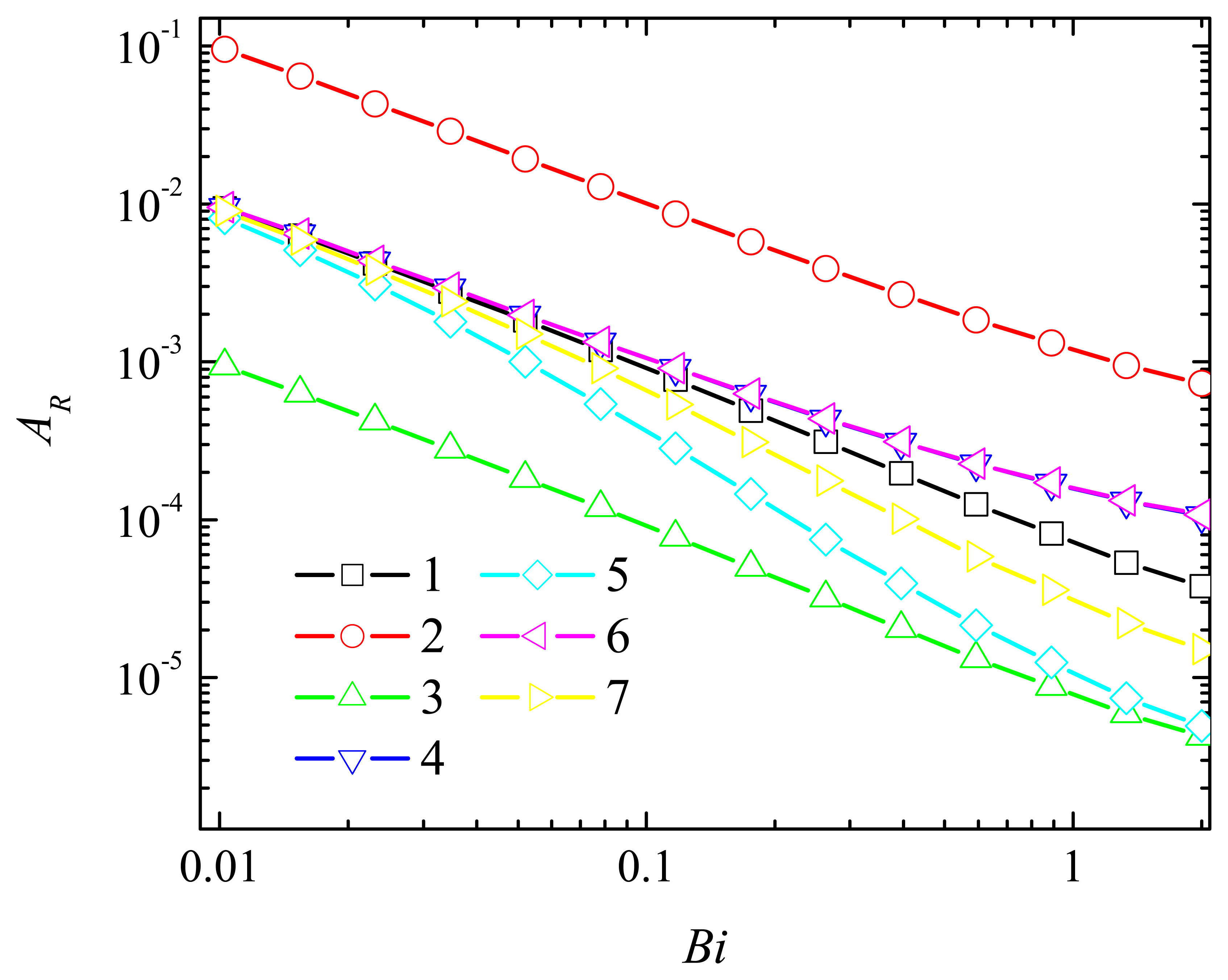
Figure 8.
Dependence of the half time T0.5 of the steady state response on the Biot number Bi at a constant thickness d = 1μm of the enzyme layer. The parameters and notation are the same as in Fig. 7.
Figure 8.
Dependence of the half time T0.5 of the steady state response on the Biot number Bi at a constant thickness d = 1μm of the enzyme layer. The parameters and notation are the same as in Fig. 7.
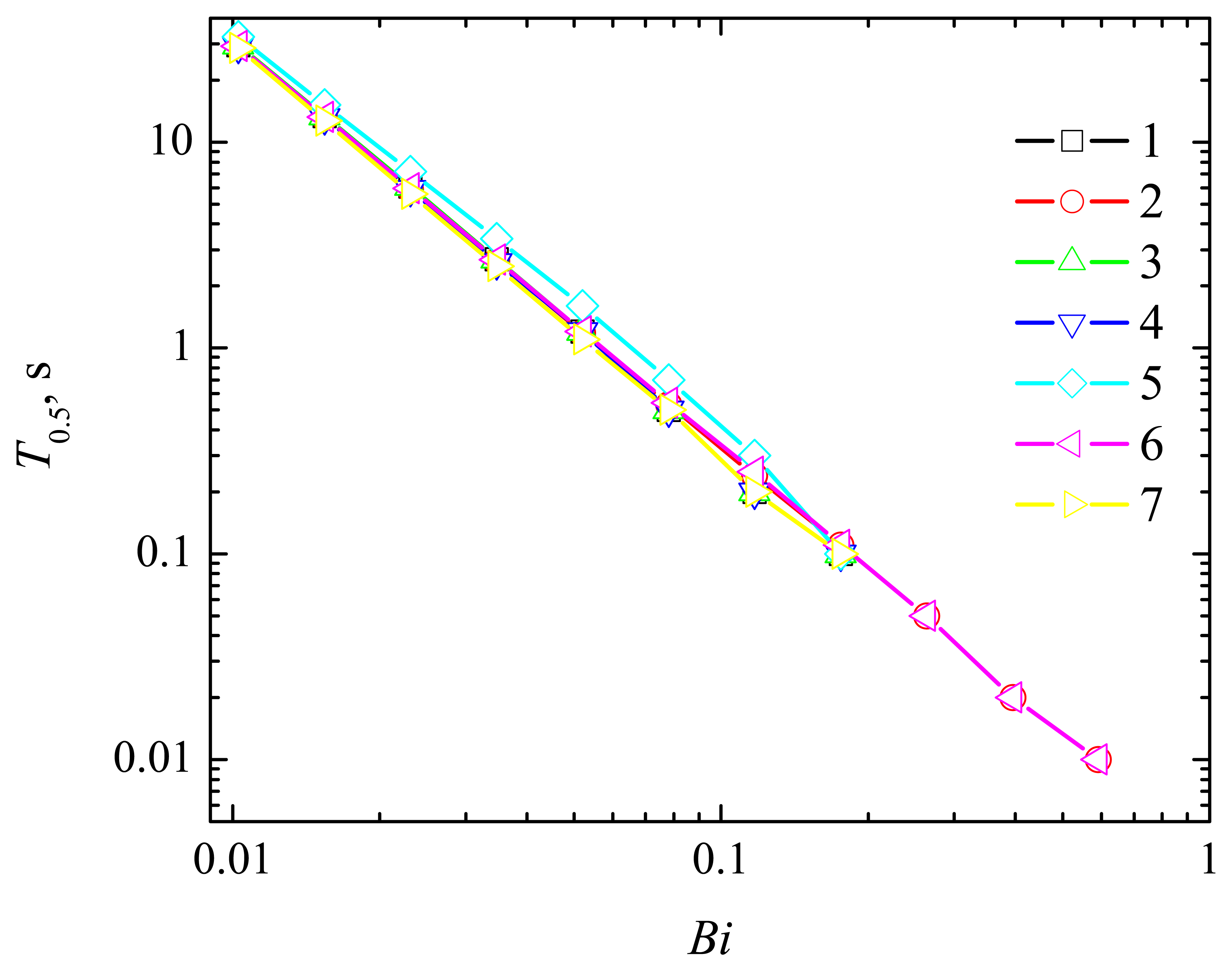
Figure 9.
Dependence of dimensionless sensitivity BS on the Biot number Bi at a constant thickness d = 1μm of the enzyme layer. Calculation parameters and notation are the same as in Fig. 7.
Figure 9.
Dependence of dimensionless sensitivity BS on the Biot number Bi at a constant thickness d = 1μm of the enzyme layer. Calculation parameters and notation are the same as in Fig. 7.
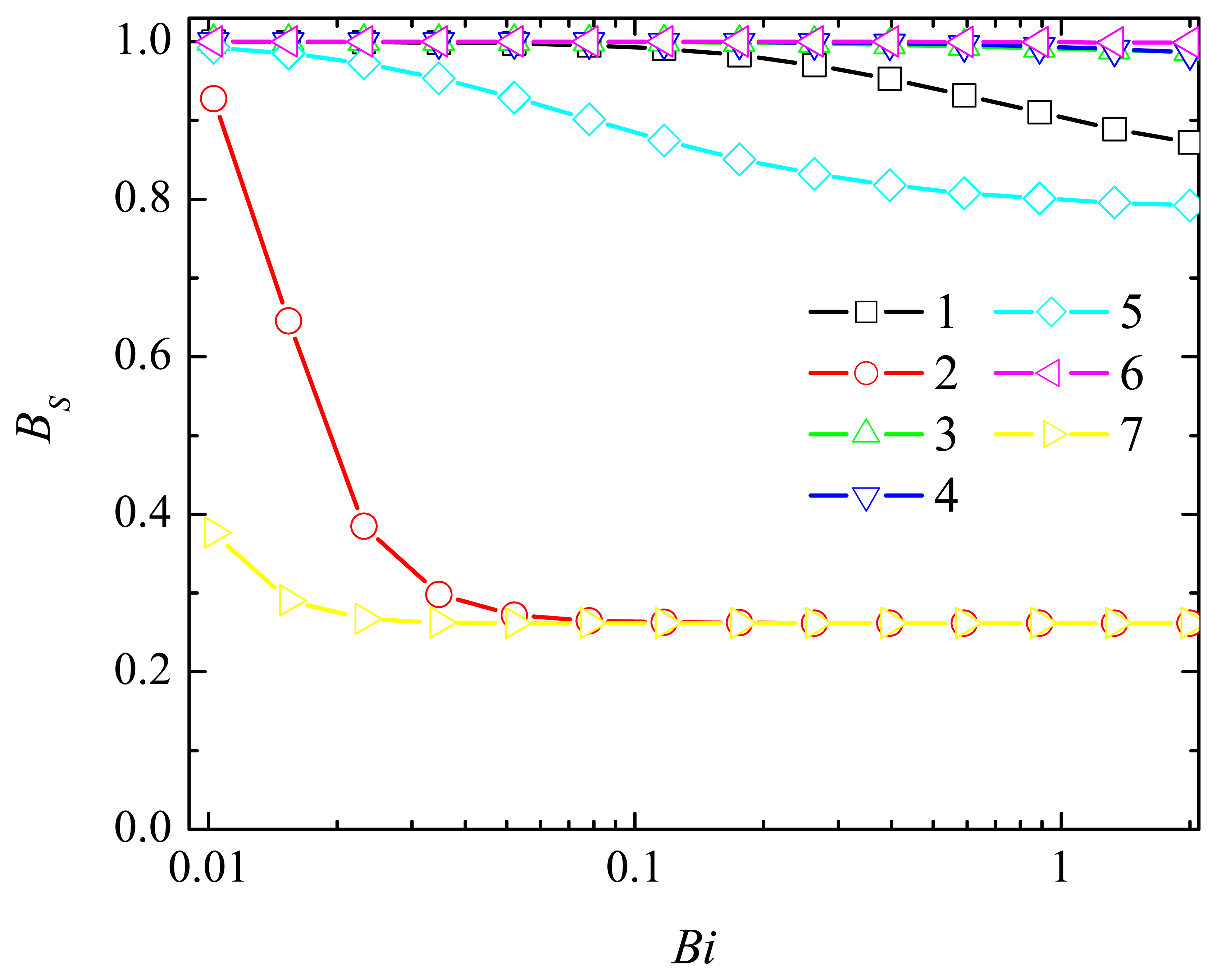
Figure 10.
Dependence of the absorbance AR on the Biot number Bi at a constant thickness δ = 100 μm of the diffusion layer. Other parameters and notation are the same as in Fig. 7.
Figure 10.
Dependence of the absorbance AR on the Biot number Bi at a constant thickness δ = 100 μm of the diffusion layer. Other parameters and notation are the same as in Fig. 7.
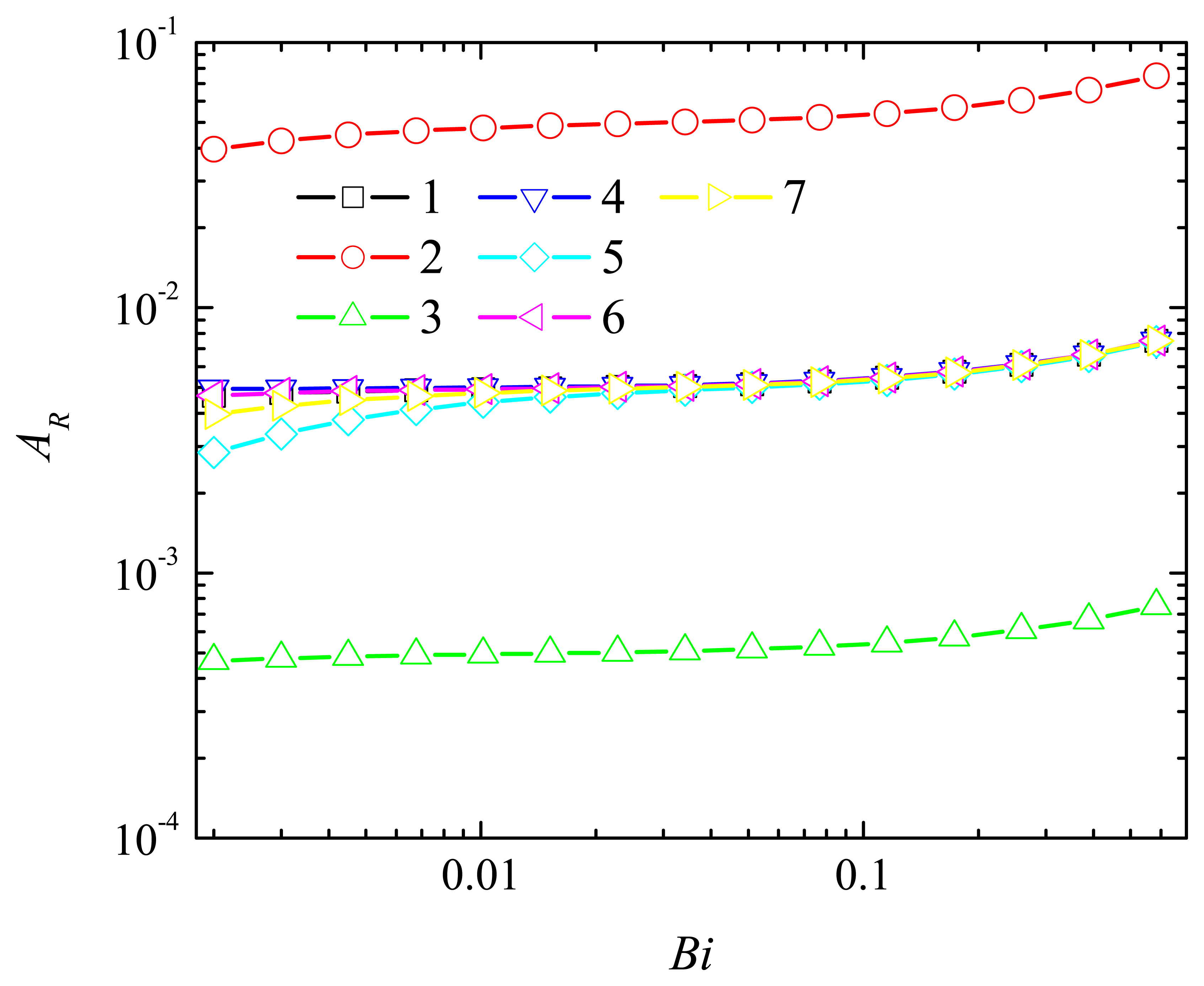
Figure 11.
Dependence of the response time on the Biot number Bi at a constant thickness δ = 100 μm of the diffusion layer. Other parameters and notation are the same as in Fig. 7.
Figure 11.
Dependence of the response time on the Biot number Bi at a constant thickness δ = 100 μm of the diffusion layer. Other parameters and notation are the same as in Fig. 7.
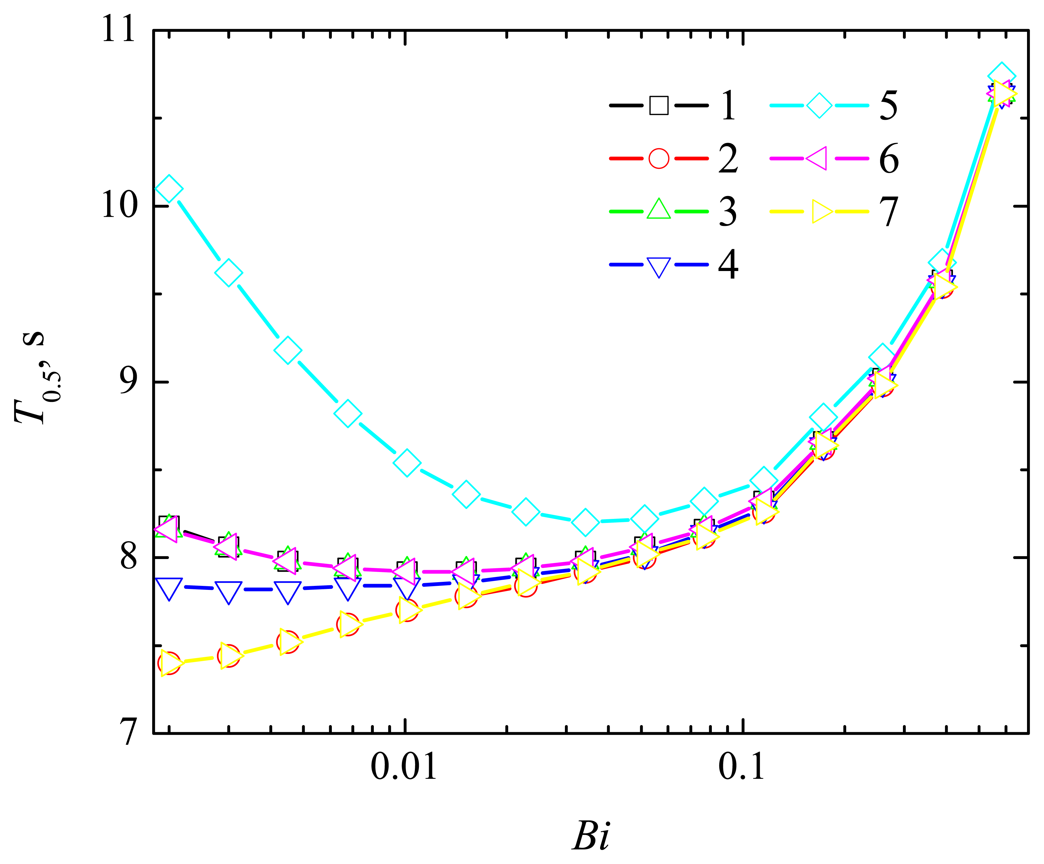
Figure 12.
Dependence of the dimensionless sensitivity BS on the Biot number Bi at a constant thickness δ = 100 μm of the diffusion layer. Other parameters and notation are the same as in Fig. 7.
Figure 12.
Dependence of the dimensionless sensitivity BS on the Biot number Bi at a constant thickness δ = 100 μm of the diffusion layer. Other parameters and notation are the same as in Fig. 7.
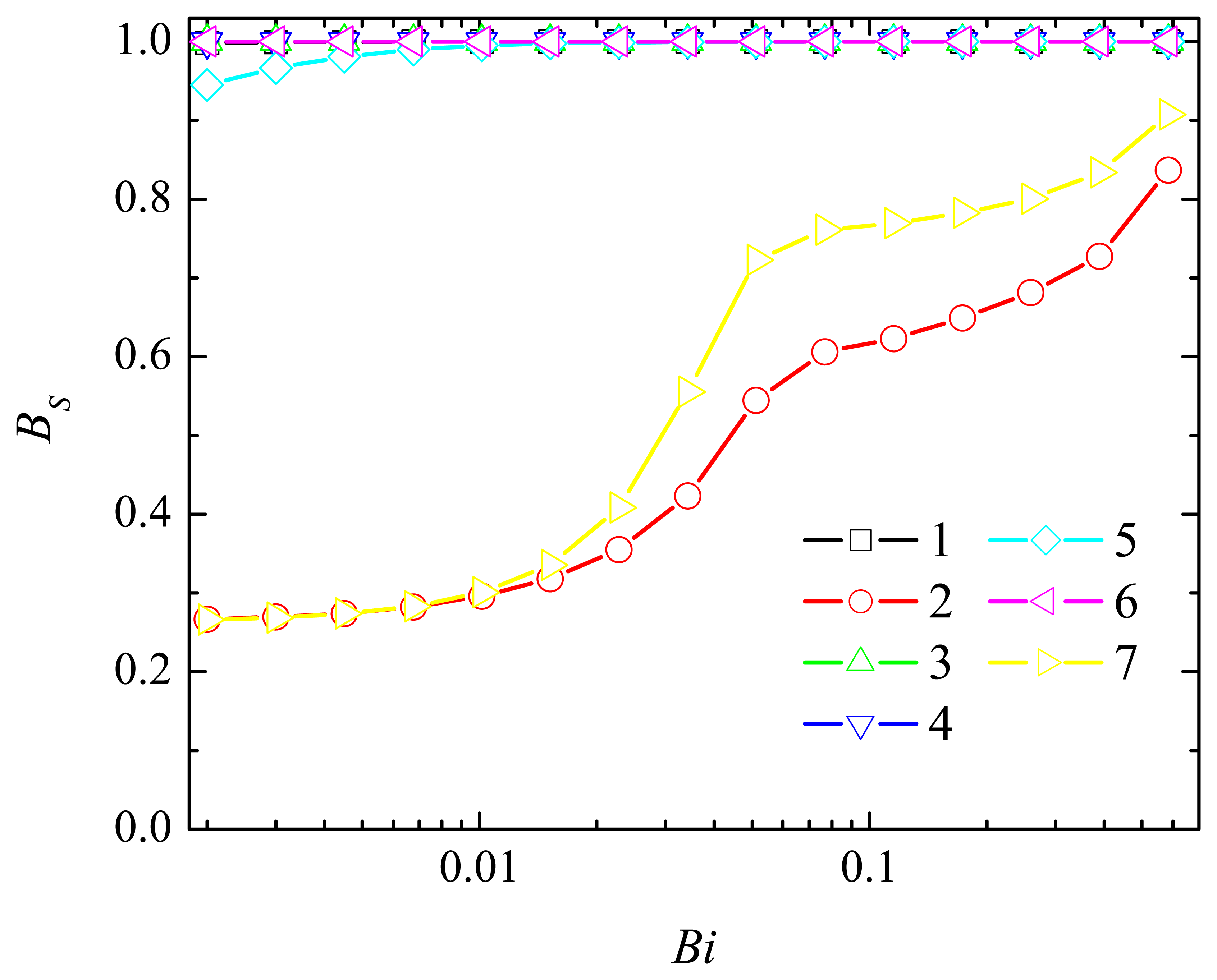
Figure 13.
Dependence of the absorbance AR on the dimensionless ratio Σ of the reactions (2) and (1) changing the substrate concentration S0 at three initial concentrations H0 of the hydrogen peroxide: 0.1 (5), 1 (1, 2, 3), 10 (4) mM and three initial concentrations E0 of the enzyme: 0.1 (3), 1 (1, 4, 5), 10 (2) nM; d = 1μm, δ = 400μm.
© 2007 by MDPI ( http://www.mdpi.org). Reproduction is permitted for noncommercial purposes.
Share and Cite
MDPI and ACS Style
Baronas, R.; Gaidamauskait˙e, E.; Kulys, J. Modelling a Peroxidase-based Optical Biosensor. Sensors 2007, 7, 2723-2740. https://doi.org/10.3390/s7112723
AMA Style
Baronas R, Gaidamauskait˙e E, Kulys J. Modelling a Peroxidase-based Optical Biosensor. Sensors. 2007; 7(11):2723-2740. https://doi.org/10.3390/s7112723
Chicago/Turabian StyleBaronas, Romas, Evelina Gaidamauskait˙e, and Juozas Kulys. 2007. "Modelling a Peroxidase-based Optical Biosensor" Sensors 7, no. 11: 2723-2740. https://doi.org/10.3390/s7112723