Lidar-based Studies of Aerosol Optical Properties Over Coastal Areas


1
Institute of Oceanology, Polish Academy of Sciences, ul. Powstancow Warszawy 55, 81-712 Sopot, Poland
2
Remote Sensing Technology Institute, DLR - German Aerospace Center, Rutherfordstr. 2, D-12489 Berlin, Germany
*
Author to whom correspondence should be addressed.
Sensors 2007, 7(12), 3347-3365; https://doi.org/10.3390/s7123347
Submission received: 1 November 2007
/
Accepted: 17 December 2007
/
Published: 19 December 2007
(This article belongs to the Special Issue Ocean Remote Sensing)
Abstract
:Aerosol size distribution and concentration strongly depend on wind speed, direction, and measuring point location in the marine boundary layer over coastal areas. The marine aerosol particles which are found over the sea waves in high wind conditions affect visible and near infrared propagation for paths that pass very close to the surface as well as the remote sensing measurements of the sea surface. These particles are produced by various air sea interactions. This paper presents the results of measurements taken at numerous coastal stations between 1992 and 2006 using an FLS-12 lidar system together with other supporting instrumentation. The investigations demonstrated that near-water layers in coastal areas differ significantly from those over open seas both in terms of structure and physical properties. Taking into consideration the above mentioned factors, aerosol concentrations and optical properties were determined in the marine boundary layer as a function of offshore distance and altitude at various coastal sites in two seasons. The lidar results show that the remote sensing algorithms used currently in coastal areas need verification and are not fully reliable.
1. Introduction
Aerosol properties in marine boundary layers over regional seas and coastal environments vary from those in open ocean regions. Sea spray particle production in coastal areas is enhanced at the sea surface mainly due to wave breaking and generation by onshore winds, while offshore winds carry particles of continental, often anthropogenic origin. Thus, the ensemble of aerosol particles in the marine boundary layer over the coastal area, depending on the air mass history, can be comprised of a majority of sea salt particles or a mixture of both types of particles [1-3].
Coastal areas as sources of marine aerosols play important roles due to the fact that breaking waves occur in this area even at small wind speeds. Breaking waves create whitecaps and sea-spray droplets which consist of a large number of air bubbles essential for greater production of marine aerosols [4-5]. Concentration of air bubbles in breaking waves is four times higher in the surf zone than in the ocean under the same weather conditions. Sea-spray droplets and droplets from bursting bubbles elevated into the marine boundary layer constitute marine aerosols [5-8]. Such mechanisms and sources of marine aerosols are well described theoretically and well investigated experimentally [4, 8]. Based on results of many research findings, models have appeared dealing with problems of dependence of marine aerosol generation, transport and deposition from the marine boundary layer on various physical parameters of the atmosphere [9-11]. Especially well described is the dependence of wind speed on concentration and size distribution of marine aerosol over the ocean. Such models, however, can not be directly applied to coastal areas for which the amount and quality of data collected are insufficient.
2. Description of experiments and instrumentation
The lidar based measurements were taken from several stations on the Baltic Sea coast between 1992 and 2006. Simultaneous values of aerosol optical thickness obtained from the FLS-12 lidar and CIMEL C-318 sunphotometer were recorded during measurements taken in Duck, NC on the Atlantic coast of the USA during an international campaign EOPACE (Electrooptical Propagation Assessment in Coastal Environments) which was conducted between 25 February and 11 March 1999. Location of measurement stations on the Baltic coast are illustrated in Figure 1.
The measurement stations are located east of 17°30′E. The fetch length at these stations is up to 300-400 Nm, which with onshore winds secures the marine aerosol conditions. Two wind direction regimes, onshore and offshore were taken into consideration. Conditions were classified as “onshore” when the wind blew onshore for at least eight hours prior to the measurement session. Additionally, the air mass back trajectories were checked to ensure that the onshore conditions using the BADC service ( http://badc.nerc.ac.uk/home/index.html) had been properly classified. Each measurement campaign lasted from 3 to 14 days, and each measurement session lasted from 7 to 16 hours, depending on weather conditions. Wind speed and direction and wet and dry-bulb temperatures were recorded along with other supporting information during all the campaigns. The full description of the meteorological parameters registered during the measurement campaigns in the Baltic area are presented in Table 1 [12].
The data presented in Table 1 show that the experiments were carried out in spring (7) and in fall (6). Both spring (early summer) and fall are optimal seasons in the Baltic for aerosol measurements. April, May, June and September are months of statistically lowest cloud coverage (conditions good for aerosol optical properties measurements) while the highest wind speeds in the area (increased marine aerosol production) are measured in March, September, October and November [13-14]. Table 2 presents the data regarding the number of experiments in spring and fall and days with onshore winds over a period of 1992 – 2006.
The data presented in Table 2 include only selected days with clear situation regarding the wind direction using the criteria described above. Basic meteorological parameters measured during the EOPACE experiment in Duck, NC in 1999 are presented in Table 3 [12].
The lidar system FLS-12 was used to take aerosol concentration measurements at the shore stations and was installed in a van and deployed on the top of the dunes at a fixed distance from the sea [15]. The inclination of the lidar is easy to adjust, which allowed the marine boundary layer to be sounded at various altitudes. In Duck, NC the lidar was placed at the very end of the measurements pier (c. 700 m length) right next to a CIMEL instrument.
The lidar FLS-12 is a tunable laser system designed for remote sensing of the air in the VIS spectrum range (320-670 nm). The source of UV pumping for the dye laser is a XeCl excimer laser (308 nm). During the experiments the lidar collected aerosol backscattered data every 50 ns, that is every 7.5 m on the optical path, and three wavelengths of 430 nm, 560 nm and 670 nm were employed. The useful part of the optical path was between 60 and 2000 m and altitudes up to 500 m were sounded. A detailed description of the FLS-12 lidar and the measurement methodology can be found in [16].
The inclination of the lidar was easily changed, which allowed for sounding the marine boundary layer at various altitudes ranging from h = 1 m above sea level to vertical profiling of the marine boundary layer. The aerosol concentrations were determined over the surf zones. The principal parameters of the lidar FLS-12 are presented in Table 4 [16].
The lidar-obtained aerosol concentrations were calibrated with those obtained from simultaneous measurements with a laser particle counter (CSASP-HV-100-SP) which was mounted at different distances along the lidar sensing path and in several cases also with six cascade impactors [17].
3. Methodology of lidar measurements
The aerosol concentration at an arbitrary altitude above sea may be determined using the Potter procedure [18] and the Mie algorithm, if a predetermined function is assumed. This procedure allows for the determination of the extinction at an arbitrary point zi located on the sounding path with lidar radiation of wavelengths λ1 and λ2. The extinction εij derived at an arbitrary point zi from the back scattered lidar radiation of wavelength λj can be expressed as follows:
where r is a particle radius, Q(r, λj) is the extinction efficiency in the Mie theory and n(r, zi, hi)is the aerosol size distribution function.
For aerosol particles of marine origin (non-absorbing spherical water droplets) function n(r, zi, hi) may take the following form [19]:
where a, b > 0 are distribution parameters.
Dependence (2) can also be applied to the description of continental aerosol and the mixture of two aerosol types: continental and marine. This, however, requires information about the contribution of particular types of particles and their optical properties (refraction indexes) or simultaneous investigations aimed at the calibration of aerosol concentrations obtained from the lidar. Non-linear minimization was used to determine the values of distribution parameters a and b which best fit formula (1).
These parameters determine the size distribution and total aerosol concentration at point zi and altitude hi as follows:
where Nr(zi, hi) is the number concentration of aerosol particle in the size range r, r + dr. Function f(r) is a normalized size distribution function:
Where: b is a parameter [1/μm].
In dependence (3) the values of r1 and r2 must be selected in such a way so that the lidar measurements allow for the determination of the aerosol concentration Nc at an arbitrary point zi with minimum error. It is a complex problem since in both study areas, Duck, N.C. and the southern Baltic Sea, the aerosol particles have different optical properties and, depending on the wind direction, their ensemble consists of either a mixture of continental and marine particles (absorbing particles) or marine particles (non-absorbing particles). In each case, the values of the refraction indexes are different due to the difference of salinity of the surface waters (Duck, NC - S ≅ 36 PSU, Baltic - S ≅ 8 PSU) and the different chemical composition of the continental aerosol [20-25].
Therefore, the question arises if the r1 and r2 from dependence (3) have the same values for aerosol which consists of particles of various optical properties which are described by the same size distribution function f(r). This problem can be solved through the theoretical determination of the shape of function Q(r, λ) f(r) from formula (1). The assumption that parameter b of the size distribution function is constant (b = 2) facilitated the derivation of function Q(r, λ) f(r) for spherical, absorbing particles of the light refraction index m = 1.48 – i 0.01; m = 1.4 – i 0.01 and non-absorbing particles of m = 1.338 and m = 1.353 for radiation of two wavelengths, λ1 = 400 nm and λ2 = 700 nm [24]. The light refraction indexes assumed for the non-absorbing spheres are the boundary values of these parameters for waters of salinity S = 36 PSU (Duck, NC) and S = 8 PSU (Baltic Sea) at temperatures of T = 1 °C and T = 15 °C. The most commonly used values for a mixture of continental and marine particles were applied for absorbing particles. It has been showed that aerosol particles of sizes r < 0.5 μm (absorbing and non-absorbing) have a small impact (< 5 %) on the backscattered signal (especially for λ = 400 nm), while particles of sizes r > 5 μm are too few to have a significant impact on light absorption and scattering (< 1 %) [26]. Therefore, the concentrations derived in the coastal area using the lidar method for particles from the range of radii r ∈ [0.5 μm, 5 μm] are loaded with small error, which has an insignificant impact on the extinction values. Therefore, formula (3) for this range of radii can be written as follows:
Values of parameter b(zi, hi) in dependencies (5) and (6) depend on wind speed and direction as well as the sea bottom slope in the coastal area [15]. In the coastal area of the southern Baltic Sea the value of this parameter for various wind speeds and directions varies in the following range of b ∈ [2, 2.6] [27]. In the case of Duck, NC, the value of b = 2 1/μm was accepted which relates to the maximum of the distribution function for particles of rm = 2/b = 1 μm.
Knowledge of aerosol concentrations and size distribution function facilitates the analysis of the impact of the meteorological conditions on the value of the aerosol extinction coefficient εA (z, λ), which is described as follows:
The analyses of coefficients εA (z, h, λ) as functions of meteorological parameters were carried out for the mean values of the Mie coefficients as follows:
Formula 1 indicates that the aerosol extinction also depends on the dimensionless extinction coefficient Q. The values of this coefficient were derived by taking different types of aerosol (wind direction) into consideration for different light refraction indexes and different wavelengths. The distribution parameters a and b were derived for different values of Q and different light refraction indexes and wavelengths. The authors agree that the continental aerosol includes more particles of a radii r<0.5 μm. However, the calculations of the Q coefficient for aerosol particles of m=1.48-i0.01 and radius r = 0.5 μm give the following values of Q [12]:
- Q = 1.4·10-12 m2 for λ=400 nm
- Q = 3.36·10-12 m2 for λ=700 nm
While for particles of radii r=0.1 μm and r=0.02 μm the Q values are as follows:
- Q = 2.2·10-14 m2 for λ=400 nm
- Q = 3.87·10-15 m2 for λ=700 nm
- Q = 2·10-18 m2 for λ=400 nm
- Q = 2.3·10-19 m2 for λ=700 nm
These values are very low, and, despite the large number of these particles, their influence on the aerosol extinction in the VIS is relatively insignificant. The laser beam is deflected off of these particles, not backscattered, thus the lidar does not register them.
For particles of a radii r>5 μm, the Q values are high but their contribution to the extinction is low due to their small number. Additionally, the value of the aerosol extinction obtained from the lidar method is loaded with 30% error, thus it is assumed that this error also includes the error which results from omitting particles sizes r<0.5 μm and r>5 μm.
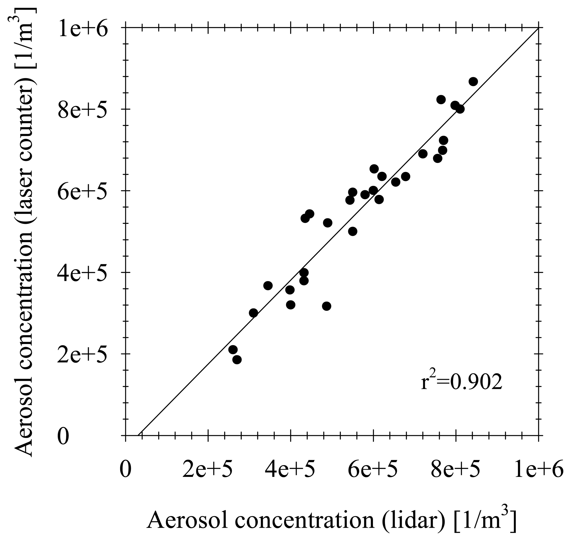
The comparison of the FLS-12 lidar concentrations with those obtained simultaneously using the CSASP-HV-100-SP at different coastal stations of the southern Baltic coast between 1993 and 2000 are presented in Figure 2 [17, 28]. Data were recalculated to relative humidity conditions of 80%.
The results presented in Figure 2 show good correlation of data obtained from both instruments - (r2 = 0.902). Detailed information regarding the calibration of measurements made with FLS-12 lidar and CSASP-100-HV-SP laser counter are given in [29].
The aerosol optical thickness τA was determined as a function of visibility in the analytical form as follows [30]:
where: λ - light wavelength [nm]; H1 = 0.886 + 0.0222 V(λ) [km] and H2 = 3.77 km;
- horizontal visibility [km].
4. Results and discussion
Aerosol optical properties change with the change of their origin. The authors assumed that the light absorption coefficient in the visible range of light is close to zero for marine particles. Thus the marine aerosol particles have only scattering properties. In case of the offshore winds such assumption could not be made.
Aerosol extinction coefficients obtained from the FLS-12 lidar measurements at 550 and 670 nm in Duck, NC and at the Baltic stations are presented in figure 3.
The aerosol extinction coefficients are higher in Duck, NC with offshore winds than in Lubiatowo, while for onshore winds, at the range of wind speeds from 2 to 14 m/s the aerosol extinction coefficients are comparable in both cases. In order to show the differences in aerosol extinction coefficients at various altitudes Table 5 shows the lidar and laser particle counter results obtained at different altitudes in Duck, NC and in Lubiatowo.
In all cases presented in Table 5 the aerosol extinction coefficient measured at 4 m a.s.l. is higher than that measured at 30 m a.s.l., which results from higher aerosol concentrations (especially coarse mode) near the sea surface. Higher concentrations of marine aerosol particles in Duck, NC result from higher water salinity and about 4 times wider surf zone. However, for both wind directions the values obtained from the lidar studies at 30 m a.s.l. in Duck, NC are lower than the analogous results obtained at the Baltic station. This may have resulted from the fact that larger particles (S=36 PSU) in Duck, NC fall down faster and do not reach higher altitudes as easily as smaller particles (S=8 PSU) from the Baltic. Table 6 presents the results of a comparison of aerosol extinction coefficients reported by different researchers from different areas as well as model data [12].
The data presented in the table show a large difference in values reported by different researchers and used in different models. It is evident that the model values and the values from over the open sea differ from those obtained at the coastal stations. The comparable values obtained from the lidar at 30 m a.s.l. with those from the OPAC model (entire atmospheric column) suggest that the marine boundary layer in the coastal area (for coarse mode particles) has a dominating role in light extinction.
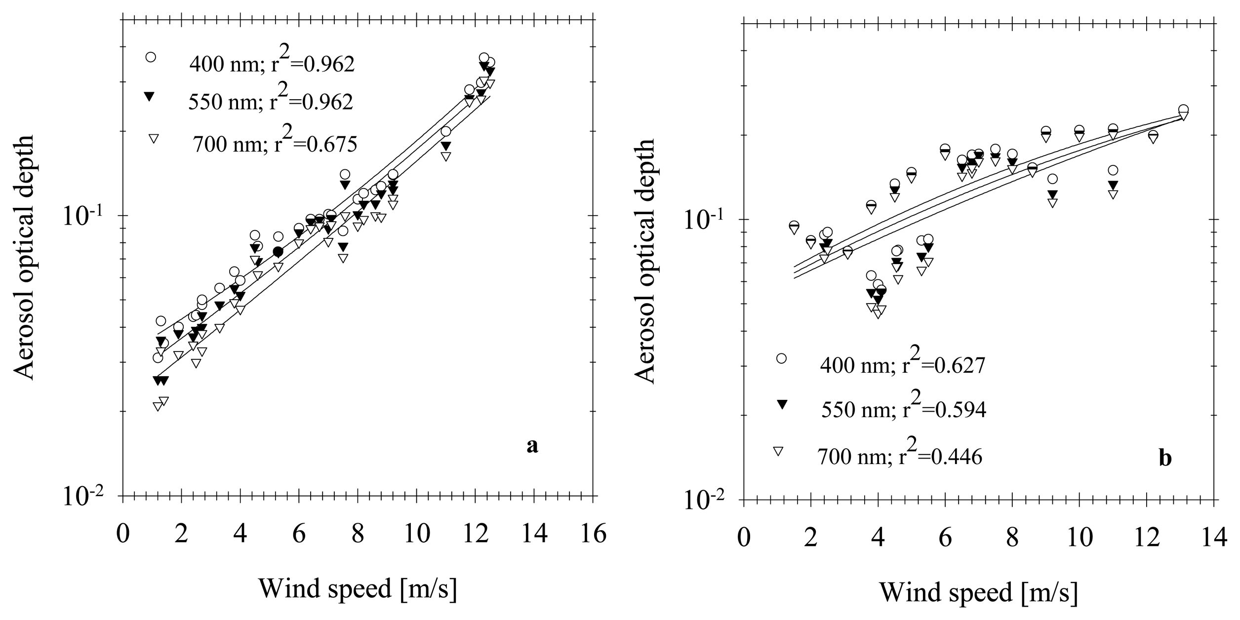
Figure 4 presents the variations of aerosol optical depth with wind speed at the coastal site in Lubiatowo on the Baltic Sea.
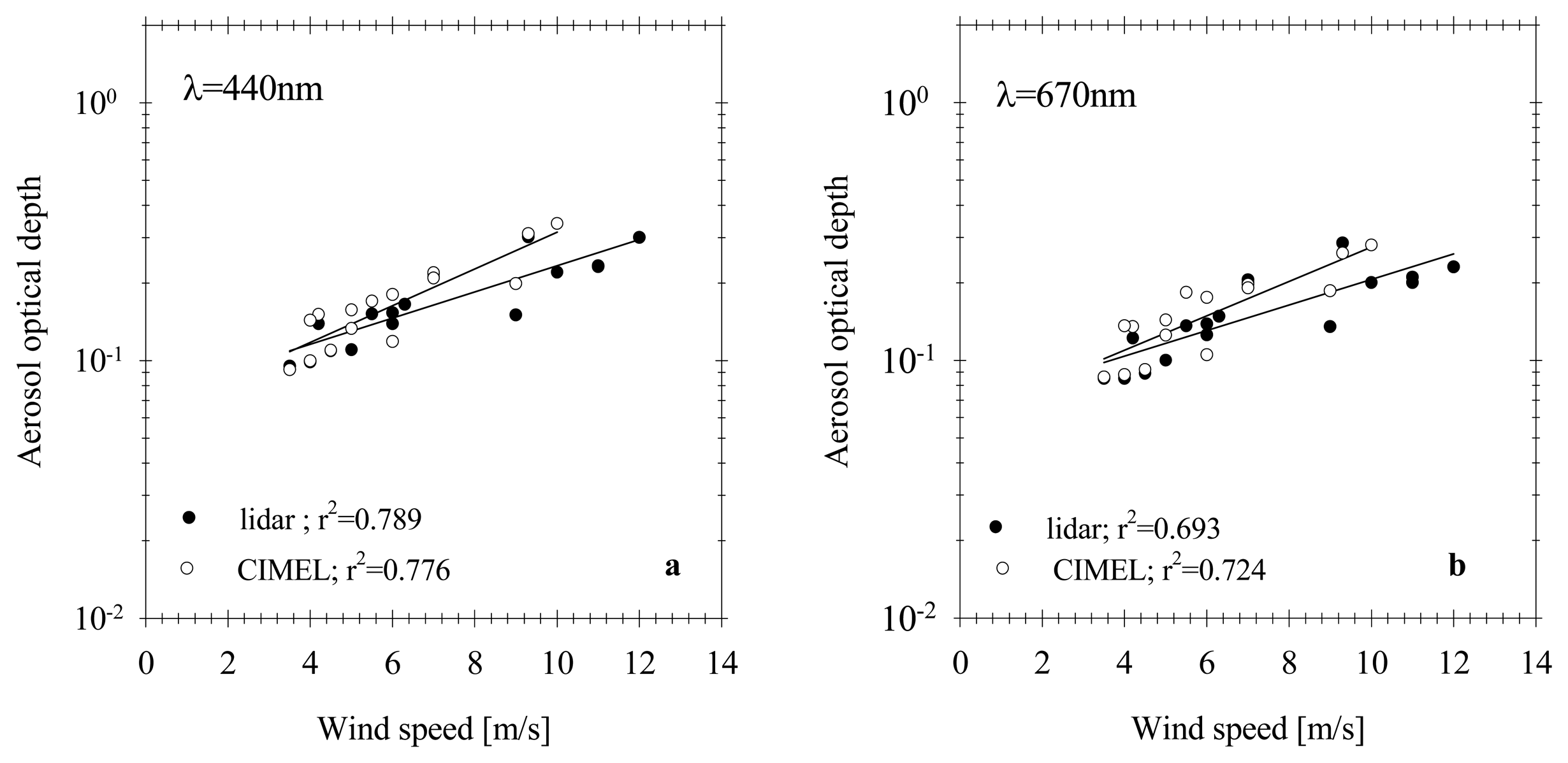
AOD values obtained for offshore winds are higher than those obtained for onshore winds and at wind speeds below 5 m/s this difference can reach half an order of magnitude. During the EOPACE experiment in Duck, NC the direct AOD measurements were made using CIMEL CE-318-1. One of them was placed right next to the FLS-12 lidar at the end of the pier. Figure 5 presents the comparison of the AOD data obtained simultaneously with the FLS-12 lidar and CIMEL CE-318-1 [12].
In both cases at wind speeds v<7m/s the AOD values obtained from the sunphotometer are slightly higher than those obtained from the lidar. The differences vary from 2.6% (v=4 m/s) to 12% (v=5.5 m/s) for onshore winds and from 1.3% at v=6m/s to 4% at v=5.5 m/s for offshore winds. The lidar data were collected (particle sizes r∈[0.5, 5 μm]) at altitudes from about 10 m to about 150 m a.s.l. This means that in the lower altitudes of the marine boundary layer of the coastal zone enhanced marine aerosol production due to wave breaking plays a decisive role in the AOD levels measured. The CIMEL CE-318-1 sunphotometers measure in the entire atmospheric column, in all size ranges and thus the AOD values must be higher than in the case of the values obtained using the FLS-12 lidar. However, a very small difference in the AOD levels measured using both instruments indicates that the coarse mode marine aerosols play a decisive role in the marine boundary layer of the coastal zone [12, 37]. Table 7 presents the average AOD values obtained for the coastal zones of the southern Baltic.
The data presented in Table 7 indicate that in the ranges of prevailing wind directions in the coastal area of the southern Baltic the AOD values are significantly lower in spring (prevailing onshore winds) than in fall (prevailing offshore winds). Table 8 presents the comparison of the AOD levels obtained in the coastal areas of the southern Baltic and the values obtained by other researchers in different regions [12].
The lidar based values (at 8 m/s) for the Baltic are similar to the AOD values obtained for the Baltic by other researchers. However, the AOD value obtained by the authors (0.21) is lower than those obtained by Weller and Leiterer and von Hoyningen-Heune and Wendisch. The studies by those authors were carried out in the south-west and central Baltic, i.e. areas affected by the advection of continental particles. In case of Duck, NC (Atlantic) the AOD values are comparable with those obtained by Hoppel et al. (1990) and Reddy et al. (1990). They are also higher than the value obtained for the Greenland Sea. The results reported by Smirnov et al. (2006) are similar to those obtained by the authors in the Greenland Sea and by Hoppel et al. (1990) in the Atlantic area.
The differences in the AOD values presented in Table 8 may result from different measurement methods and different instruments applied as well as differences in meteorological conditions.
5. Comparison of aerosol retrieval from space with the ground-truth results
The atmospheric ground-truth data obtained during the BALTIRS campaigns at the coastal stations in the area of the southern Baltic were used for validation of remote sensing algorithms. This validation is realized by comparing the aerosol properties estimated from the MOS-data with the corresponding ground-truth values. Images of the AOD have been made using the PCI and the Angström-Inversion algorithms [46]. The Angström-Inversion algorithm additionally yields Angström-Exponent values. The atmosphere was sufficiently homogenous at the ground-truth measurement locations to facilitate the 5×5 pixel area over the sea, which gave unique values for comparison.
Tables 9 and 10 summarize the validation results for both algorithms [12]. The agreement between aerosol optical thickness and the Angström-Exponent estimated from the MOS-data and from the ground-truth values confirms the expectations and corresponds to results of earlier ground-truth campaigns. With regard to the Angström-Exponent retrieval theoretical considerations show that the error of the Angström-Exponent estimation increases with the decrease of AOD. Clearly, the very low AOD observed on the 23rd September is too small for reasonable Angström-Exponent estimation.
6. Conclusions
The data presented in the paper show that the aerosol optical properties in the marine boundary layer of the coastal areas differ from those over the open ocean. They are different at different coastal stations, depending on the “purity” of marine aerosol advections with air masses. They also differ from those obtained in the marine boundary layer over the open ocean. This confirms that the coastal areas are unique and that the aerosol physical properties in such areas must be very well determined and that the application of the models for open ocean yields significant errors in algorithms, e.g. atmospheric correction algorithms in remote sensing surveys.
Since marine aerosol generation in coastal areas mostly depends on wave breaking for better parameterization of the generation process it is necessary to secure wave measurements, using e.g. imagery methods. In this paper such analyses were not included since such studies were not made in the Baltic area. Additionally, the wave breaking depends on the sea bottom type. Again such information has not been included in the paper since the authors did not manage to obtain such information regarding the Duck, NC area.
Acknowledgments
This research has been partly made within the framework of an ACCENT Project SOAP and partly within the scope of the Polish National Grant MACS/AERONET/59/2007.
References and Notes
- Vignati, E.; deLeeuw, G.; Berkowicz, R. Modeling coastal aerosol transport and effects of surf-produced aerosols on processes in the marine atmospheric boundary layer. J. Geophys. Res. 2001, 106(D17), 20225–20238. [Google Scholar]
- Dubovik, O.; Holben, B.; Eck, T.F.; Smirnov, A.; Kaufman, Y.J.; King, M.D.; Tanre, D.; Slutsker, I. Variability of absorption and optical properties of key aerosol types observed in worldwide locations. J. Atmos. Sci. 2002, 59(3), 590–608. [Google Scholar]
- Zhuang, G.S.; Huang, R.H.; Wang, M.X.; Zhou, Q.; Guo, J.H.; Yuan, H.; Rao, Z. M. Great progress in study on aerosol and its impact on the global environment. Progress in Natural Science 2002, 12(6), 407–413. [Google Scholar]
- Monahan, E.C.; Mac Niocall, G. Oceanic whitecaps and their role in air-sea exchange processes; D. Reidel Publ. Comp.: Dortrecht, Holland, 1986; p. 129. [Google Scholar]
- Resch, F.J.; Darozzes, S.J.; Afeti, G. M. Marine liquid aerosol production from bursting of air bubbles. J. Geophys. Res. 1986, 91, 1019–1029. [Google Scholar]
- Blanchard, D.C.; Syzdek, L.D. Film drop production as a function of bubble size. J. Geophys. Res. 1988, 93, 3649–3654. [Google Scholar]
- Wu, J. Bubbles in the near-surface ocean. A general description. J. Geophys. Res. 1988, 93, 587–590. [Google Scholar]
- Wu, J. Comment on film drop production as a function of bubble size by D. C. Blanchard and Syzdek. J. Geophys. Res. 1990, 95, 7389–7391. [Google Scholar]
- Fairall, C.W.; Davidson, K.L.; Schacher, G.E. An analysis of the surface production of sea-salt aerosols. Tellus. 1983, 33B, 31–39. [Google Scholar]
- Fitzgerald, W.J. Marine aerosols: A review. Atmos. Environ. 1991, 25A(3/4), 533–545. [Google Scholar]
- Gong, S.L.; Barrie, L.A.; Blanchet, J.P. Modelling sea-salt aerosols in the atmosphere. J. of Geophys. Res. 1997, 102(D3), 3805–3818. [Google Scholar]
- Zielinski, T. Physical properties of aerosol near-water layer in coastal areas. Rozprawy i Monografie IOPAN 2006, 18, 164, in Polish. [Google Scholar]
- Mietus, M.; Owczarek, M. Meteorological conditions. In Environmental conditions in the Polish area of the Baltic Sea in 1997; Cyberska, B., Lauer, Z., Trzosinska, A., Eds.; Materiały Oddziału Morskiego IMGW, 1998; Gdynia; pp. 9–31, in Polish. [Google Scholar]
- Mietus, M.; Filipiak, J.; Owczarek, M. Meteorological condition. In Environmental conditions in the Polish area of the Baltic Sea in 2000; Krzyminski, W., Lysiak-Pastuszak, E., Mietus, M., Eds.; Materiały Oddziału Morskiego IMGW, 2001; Gdynia; pp. 9–32, in Polish. [Google Scholar]
- Zielinski, T.; Zielinski, A.; Piskozub, J.; Drozdowska, V.; Irczuk, M. Aerosol optical thickness over the coastal area of the southern Baltic Sea. Optica Applicata. 1999, 29(4), 339–447. [Google Scholar]
- Zielinski, T.; Zielinski, A. Aerosol extinction and optical thickness in the atmosphere over the Baltic Sea determined with lidar. J. Aerosol Science. 2002, 33(6), 47–61. [Google Scholar]
- Zielinski, T. Changes in aerosol concentration with altitude in the marine boundary layer in coastal areas of the southern Baltic Sea. Bull. PAS. Earth Sci. 1998, 46(3-4), 133–139. [Google Scholar]
- Potter, J. Two-frequency lidar inversion technique. Appl. Opt. 1987, 26(7), 1250–1256. [Google Scholar]
- International Association for Meteorology and Atmospheric Physics, Radiation Commission. A preliminary cloudless standard atmosphere for radiation computation; Boulder, USA, 1984; pp. 9–10. [Google Scholar]
- Hoppel, W.A.; Frick, G.M.; Larson, R.E.; Mack, E.J. Aerosol size distributions and optical properties found in the marine boundary layer over the Atlantic Ocean. Journal of Geophys. Res. 1990, 95, 3659–3686. [Google Scholar]
- O'Dowd, C.D. On the spatial extent and evolution of coastal aerosol plumes. Journal of Geophys. Res. 2002, 107(D 19), 8105. [Google Scholar]
- Hegg, D.A.; Livingston, J.; Hobbs, P.V.; Novakov, T.; Russell, P. Chemical apportionment of aerosol column optical depth off the mid-Atlantic coast of the United States. J. Geophys. Res. 1997, 102, 25293–25303. [Google Scholar]
- Quinn, P.K.; Coffman, D.J.; Bates, T. S.; Miller, T.L.; Johnson, J. E.; Voss, K.; Welton, E. J.; Neusüss, C. Dominant aerosol chemical components and their contribution to extinction during the Aerosol 99 cruise across the Atlantic. J. Geophys. Res. 2001, 106, 20783–20809. [Google Scholar]
- Kiser, R.E. The generation and characterization of surf zone aerosols and their impact on naval electro-optical systems. M.Sc Thesis, Nav. Postgrad. Sch. Monterey, CA, 1996. [Google Scholar]
- Leeuw de, G. Sea spray production from waves breaking in the coastal zone. Journal Aerosol Sci. 1999, 30 (Suppl. 1), S63–S64. [Google Scholar]
- Zielinski, T. Studies of aerosol physical properties in coastal areas. Aerosol Science&Technology 2004, 38(5), 513–524. [Google Scholar]
- Stramska, M.; Petelski, T. Observations of oceanic whitecaps in the north polar waters of the Atlantic. J. Geophys. Res. 2003, 108(C3), 3086. [Google Scholar]
- Zielinski, T.; Petelski, T. Studies of aerosol physical properties in the coastal area. Optica Applicata 2006, 36, 629–634. [Google Scholar]
- Zielinski, T.; Zielinski, A. Breaker zone aerosol dynamics in the southern Baltic Sea. Atmospheric Propagation and Remote Sensing. Proceedings of the SPIE; 1994; Volume 2222, pp. 316–327. [Google Scholar]
- Gathman, S.G. Atmospheric electrical space charge near the ocean surface. In Oceanic Whitecaps; Monahan, E.C., Niocall, M., Eds.; D. Reidel: Norwell, MA, 1983; pp. 227–243. [Google Scholar]
- d'Almeida, G.; Koepke, P.; Shettle, E. Atmospheric aerosols. Global Climatology and Radiative Characteristics; A. DEEPAK Publishing, 1991; p. 561. [Google Scholar]
- Gathman, S.G.; Jensen, D.R. Aerosol characteristics in a coastal region (results from MAPTIP). Proc. SPIE Int. Soc. Opt. Eng. 1995, 2471, 2–12. [Google Scholar]
- Gathman, S.; Smith, M. On the nature of surf generated aerosol and their effect on electro-optical systems. Proc. SPIE Int. Soc. Opt. Eng. 1997, 3125, 2–13. [Google Scholar]
- Hess, M.; Koepke, P.; Schult, I. Optical Properties of Aerosols and Clouds: The Software Package OPAC. Bull. of the American Meteorological Society. 1998, 79(5), 831–844. [Google Scholar]
- Jensen, D.; Gathman, S.; Zeisse, C.; deLeeuw, G.; Smith, M.; Fredrikson, P.; Davidson, K. Electrooptical Propagation Assessment in Coastal Environments (EOPACE): summary and accomplishments. Opt. Eng. 2001, 40(8), 1486–1498. [Google Scholar]
- Von Hoyningen-Huene, W.; Weindisch, M. Possibility of refractive index determination of atmospheric aerosol particles by ground-based solar extinction and scattering measurements. Atmos. Environ. 1994, 28, 785–792. [Google Scholar]
- Weller, M.; Leiterer, V. Experimental data on spectral aerosol optical thickness and its global distribution. Beitr. Phys. Atmos. 1988, 61(l), 1–9. [Google Scholar]
- Schifrin, K.S.; Yershov, O.A.; Lysenko, E.L.; Volkov, B.N. Optical studies of aerosol structure over the island of Kihnu, Optical methods of studying the oceans and inland waters. K. S. Shifrin, Ed. Tallinn 1980, 244–248. [Google Scholar]
- Smirnov, A.; Villevalde, Y.; O'Neill, N.T.; Royer, A.; Tarussov, A. Aerosol optical depth over the oceans: analysis in terms of synoptic air mass types. J. Geophys. Res. 1995, 100(D8), 16639–16650. [Google Scholar]
- Kuśmierczyk-Michulec, J.; Schulz, M.; Ruellan, S.; Kruger, O.; Plate, E.; Marks, R.; de Leeuw, G.; Cachier, H. Aerosol composition and related optical properties in the marine boundary layer over the Baltic Sea. Journal Aerosol Sci. 2001, 32(8), 933–955. [Google Scholar]
- Hoppel, W.A.; Frick, G.M.; Larson, R.E.; Mack, E.J. Aerosol size distributions and optical properties found in the marine boundary layer over the Atlantic Ocean. Journal of Geophys. Res. 1990, 95, 3659–3686. [Google Scholar]
- Reddy, P.J.; Kreiner, F.W.; DeLuisis, J.J.; Kim, Y. Aerosol optical depths over the Atlantic derived from shipboard sunphotometer observations during the 1988 Global Change Expedition. Global Biogeochem. Cycles 1990, 4, 225–240. [Google Scholar]
- Pflug, B.; Krawczyk, H.; Posse, P. Atmospheric ground-truth measurements for validation of MOSdata and Angström algorithm. Proceedings of the 3rd Berlin Workshop on Ocean Remote Sensing; 1999; pp. 121–131. [Google Scholar]
- Smirnov, A.; Holben, B.N.; Sakerin, S.M.; Kabanov, D.M.; Slutsker, I.; Chin, M.; Diehl, T.L.; Remer, L.A.; Kahn, R.; Ignatov, A.; Liu, L.; Mishchenko, M.; Eck, T.F.; Kucsera, T.L.; Giles, D.; Kopelevich, O.V. Ship-based aerosol optical depth measurements in the Atlantic Ocean: Comparison with satellite retrievals and GOCART model. Geophysical Research Letters 2006, 33(14), L14817. [Google Scholar]
Figure 1.
Location of measurement stations: 1. Hel, 2. Jastarnia, 3. Chalupy, 4. Lubiatowo, 5. Leba, 6. Ustka.
Figure 1.
Location of measurement stations: 1. Hel, 2. Jastarnia, 3. Chalupy, 4. Lubiatowo, 5. Leba, 6. Ustka.
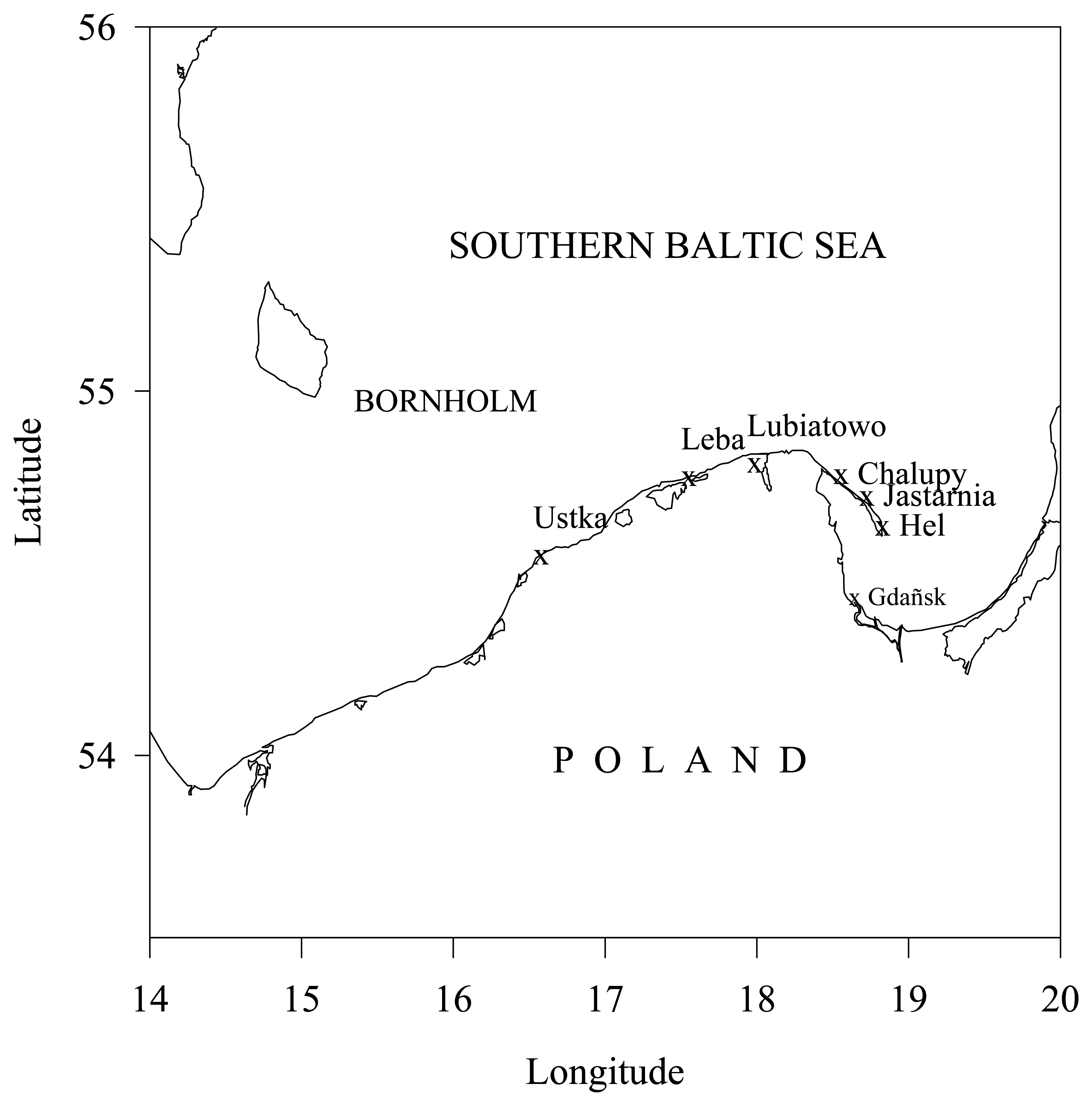
Figure 2.
Aerosol concentrations obtained from simultaneous measurements with FLS-12 lidar and CSASP-100-HV-SP laser counter.
Figure 2.
Aerosol concentrations obtained from simultaneous measurements with FLS-12 lidar and CSASP-100-HV-SP laser counter.

Figure 3.
Aerosol extinction coefficients measured with the FLS-12 lidar at 10 m a.s.l. and at 550 and 670 nm in Lubiatowo (Baltic) (a) and in Duck, NC (b).
Figure 3.
Aerosol extinction coefficients measured with the FLS-12 lidar at 10 m a.s.l. and at 550 and 670 nm in Lubiatowo (Baltic) (a) and in Duck, NC (b).
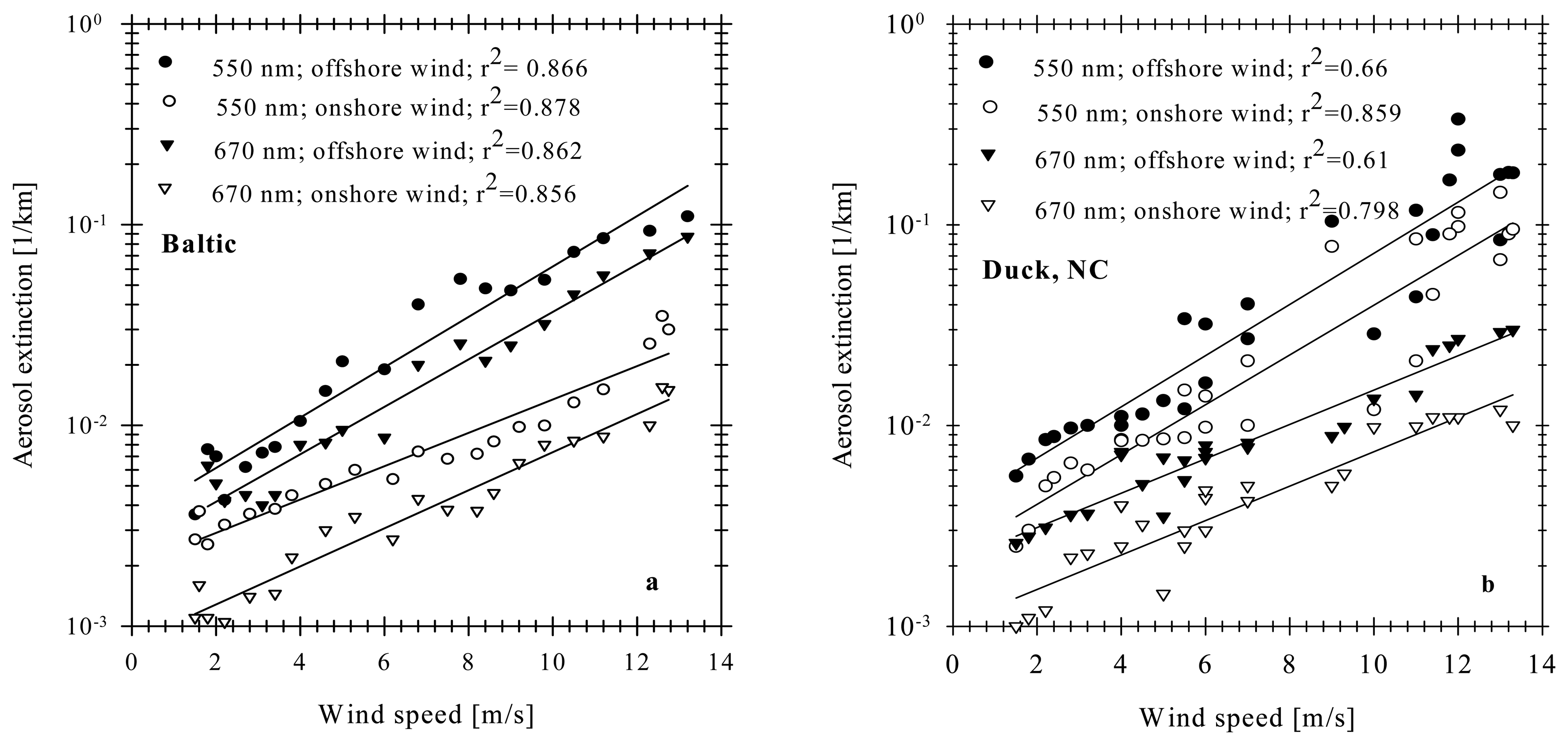
Figure 4.
Variations of aerosol optical depth on wind speed at a coastal station of Lubiatowo for onshore (a) and offshore winds (b).
Figure 4.
Variations of aerosol optical depth on wind speed at a coastal station of Lubiatowo for onshore (a) and offshore winds (b).

Figure 5.
Comparison of AOD values measured simultaneously in Duck, NC using the FLS-12 lidar and CIMEL CE-318-1 for onshore winds at 440 nm (a) and 670 nm (b).
Figure 5.
Comparison of AOD values measured simultaneously in Duck, NC using the FLS-12 lidar and CIMEL CE-318-1 for onshore winds at 440 nm (a) and 670 nm (b).


Table 1.
Description of meteorological parameters registered during the measurement sessions in the Baltic area over a period 1992-2006.
| Measurement periods 1993-2003 | Number of experiments | Prevailing wind directions | Meteorological conditions | |||||||
|---|---|---|---|---|---|---|---|---|---|---|
| T [°C] | RH [%] | p [hPa] | v [m/s] | |||||||
| Min. | Max. | Min. | Max. | Min. | Max. | Min. | Max. | |||
| March | 2 | SE | -2.6 | 5.4 | 66 | 81 | 982 | 1028 | 3.8 | 8.6 |
| April | 2 | N, NE, SW, SE | 2.3 | 9.4 | 67 | 93 | 986 | 1027 | 2.2 | 9.7 |
| May | 3 | N, NE, SW | 7.2 | 18.4 | 65 | 94 | 990 | 1032 | 2.0 | 6.8 |
| September | 2 | NE, SE, SW | 9.3 | 20.3 | 53 | 93 | 988 | 1018 | 4.6 | 11.0 |
| October | 3 | N, NE, SW, W | -2.1 | 8.6 | 62 | 96 | 990 | 1018 | 4.0 | 13.0 |
| November | 1 | SW | -2.5 | 3.2 | 55 | 78 | 1018 | 1024 | 3.1 | 12.0 |
| Total | 13 | |||||||||
| Season 1992-2006 | No. of experiments | No. of days with onshore winds | No. of days with offshore winds |
|---|---|---|---|
| Spring (late March, April, May, June) | 7 | 52 | 40 |
| Fall (September, October, November) | 6 | 22 | 60 |
| Total | 13 | 74 | 100 |
| Day in March 1999 | Meteorological conditions | ||||||||||
|---|---|---|---|---|---|---|---|---|---|---|---|
| Tw[°C] | Tp [°C] | RH [%] | p [hPa] | V [m s-1] | Wind direction | ||||||
| Min. | Max. | Min. | Max. | Min. | Max. | Min. | Max. | Min. | Max. | ||
| 1 | 5.37 | 6.25 | 4.4 | 10.5 | 51 | 72 | 996 | 1003 | 5.2 | 8.6 | Offshore |
| 2 | 4.56 | 6.80 | 7.2 | 14.4 | 52 | 68 | 1003 | 1017 | 4.2 | 7.3 | Offshore |
| 3 | 5.79 | 8.24 | 5.3 | 15.4 | 63 | 97 | 998 | 1016 | 5.8 | 8.7 | Onshore |
| 4 | 5.32 | 7.41 | 4.7 | 7.7 | 48 | 67 | 997 | 1014 | 3.0 | 9.8 | Onshore |
| 5 | 4.39 | 5.12 | 5.1 | 10.6 | 46 | 66 | 1017 | 1030 | 0.6 | 8.5 | Onshore |
| 6 | 7.20 | 8.33 | 5.1 | 17.5 | 65 | 67 | 1017 | 1028 | 3.1 | 9.2 | Onshore |
| 7 | 7.81 | 8.36 | 0.3 | 9.3 | 53 | 73 | 1015 | 1026 | 9.6 | 10.0 | Offshore |
| 8 | 6.98 | 7.45 | 0.7 | 1.6 | 66 | 76 | 1026 | 1036 | 12.1 | 13.7 | Offshore |
| 9 | 4.87 | 6.18 | 2.2 | 5.3 | 58 | 87 | 1011 | 1034 | 4.1 | 6.5 | Offshore |
| 10 | 5.1 | 6.20 | 3.4 | 5.6 | 85 | 96 | 1011 | 1015 | 3.8 | 6.4 | Offshore |
| Excimer laser | |
| Wavelength | 308 nm |
| Pulse energy | 70 mJ |
| Pulse duration | 20 ns |
| Pulse repetition | 1; 10 Hz |
| Tunable dye laser | |
| Wavelength region | 320 to 670 nm |
| Pulse duration | 15 ns |
| Efficiency of pumping energy transforming | >15 % |
| Beam divergence | < 1 mrad |
| Generation line width | < 0.1 nm |
| Receiver | |
| Spectral range | 400 to 750 nm |
| Conversion time | 50 ns |
| ADC converter | 10 bit |
| Telescope | |
| Mirror diameter | 280 mm |
| Focal length | 635 mm |
| Distances of optimal energy focusing, tunable | 10 to 2000 m |
| Polychromator | |
| Spectral region | 425 to 800 nm |
| Diffraction grating | 450 lines/mm |
Table 5.
Aerosol extinction coefficients obtained with lidar and laser particle counters (CSASP-100-HV-SP) at two altitudes in Duck, NC and Lubiatowo at the Baltic coast.
| Aerosol extinction [1/km] at λ = 550 nm | Aerosol extinction [1/km] at λ = 675 nm | |||
|---|---|---|---|---|
| Onshore wind v=7.5 m/s | Offshore wind v=5 m/s | Onshore wind v=7.5 m/s | Offshore wind v=5 m/s | |
| Lidar h=32 m Duck, NC | 0.0049 | 0.0013 | 0.0032 | 0.00098 |
| Laser counter h=4 m Duck, NC | 0.013 | 0.0098 | - | - |
| Lidar h=30 m Baltic | 0.0068 | 0.0046 | 0.0046 | 0.0028 |
| Lidar h=4 m Baltic | 0.0096 | 0.0073 | 0.0067 | 0.0057 |
| Laser counter h=4 m Baltic | 0.010 | 0.0077 | - | - |
| Author | Type of air mass | Extinction coefficient [1/km] | Study area | Description |
|---|---|---|---|---|
| Gathman, 1983 [31] | Continental | 0.370 | NAM - Navy Aerosol Model | h = 4 m a.s.l. RH = 80% v = 8 m s-1 |
| d'Almeida and Koepke, 1991 [32] | Continental Marine | 0.167 0.078 | Global Aerosol Model | Atmospheric column RH = 80% |
| Gathman and Jensen, 1995 [33] | Continental Marine | 0.58 0.04 | Coastal station Katwijk aan Zee, Holand | h = 2 m a.s.l. |
| Gathman and Smith, 1997 [34] | Marine | 0.32 | San Diego Bay, USA | h = 4 m a.s.l. RH = 80% v = 1.8 m/s |
| Gathman and Smith, 1997 [34] | Marine | 0.103 | San Diego Bay, USA | h = 8 m a.s.l. RH = 80% v = 1.8 m/s |
| Hess et al., 1998 [35] | Continental Urban Marine | 0.151 0.353 0.090 | Model OPAC-Optical Properties of Aerosols and Clouds | Atm. column h∈[0; 2000 m] RH = 80% |
| Jensen et al., 2001 [36] | Marine | 0.6 | Monterey Bay, USA | h = 4 m a.s.l. RH = 80% |
| Jensen et al., 2001 [36] | Marine | 0.1 | Monterey Bay, USA | h = 10 m a.s.l. RH = 80% |
| Zielinski, 2006 [12] | Marine (lidar) | 0.0096 | Baltic | h = 4 m a.s.l. RH = 80% v = 7.5-9 m/s |
| Zielinski, 2006 [12] | Marine (lidar) | 0.0068 | Baltic | h = 30 m a.s.l. RH = 80% v = 7.5-9 m/s |
Table 7.
The average ranges of AOD changes at RH=80% and for λ=550 nm in spring and fall calculated using the wind statistics for 1961-1990 and 1997-2000.
| Spring Onshore wind speeds, v∈[3.8, 4.8] | |
| AOD range | 0.055-0.071 |
| Fall Offshore wind speeds v∈[4.8, 6.0] | |
| AOD range | 0.144-0.174 |
Table 8.
AOD levels at 550 nm obtained by the authors for the southern Baltic stations, in Duck, NC and over the Greenland Sea. The authors' data were obtained at 8 m/s and recalculated to RH=80%.
| Author | Air mass type | AOD at 550 nm | Region |
|---|---|---|---|
| Weller and Leiterer (1988) [38] | Continental | 0.62 | Baltic |
| Marine | 0.18 | Baltic | |
| Von Hoyningen-Huene and Wendisch (1994) [37] | Continental | 0.29 | Baltic |
| Marine | 0.10 | Baltic | |
| Schifrin et al. (1980) [39] | Marine/coastal | 0.20 | Baltic |
| Schifrin et al. (1980) [39] | Marine/coastal | 0.16 | Black Sea |
| Smirnov et al. (1995) [40] | Continental/coastal | 0.33 | Black Sea |
| Kuśmierczyk-Michulec et al. (2001) [41] | Continental/mixed | >0.26 | Baltic |
| Marine | 0.26< | Baltic | |
| Zielinski (2006) [12] | Continental | 0.21 | South. Baltic coastal |
| Marine | 0.09 | South. Baltic coastal | |
| Hoppel et al. (1990) [42] | Continental | 0.13 | Atlantic |
| Marine | 0.08 | Atlantic | |
| Reddy et al. (1990) [43] | Continental | 0.50 | Atlantic |
| Marine | 0.11 | Atlantic | |
| Smirnov et al. (2006) [44] | Marine | 0.06-0.08 | South Atlantic |
| Zielinski (2006) [12] | Continental | 0.21 | Duck, NC |
| Marine | 0.11 | Duck, NC | |
| Zielinski (2006) [12] | Marine | 0.07 | Greenland Sea |
| Zielinski, 2006 | Continental | 0.22 | Crete coast |
Table 9.
The exemplary results for validation of the AOD estimation (750 nm) +/- : Variation over 5×5-Pixel ground-truth area on the sea.
| Ground-truth | PCI-Algorithm | |
|---|---|---|
| 22.09.2002 | 0.06 | 0.04 +/-0.002 |
| 23.09.2002 | 0.02 … 0.03 | 0.05 +/-0.004 |
| 27.09.2002 | 0.13 … 0.14 | 0.08 +/-0.005 |
Table 10.
Results for validation of Angström-Exponent estimation +/- : Variation over 5×5-Pixel ground-truth area on the sea
| Ground-truth | Angström-Inversion | |
|---|---|---|
| 22.09.2002 | 1.5 | 1.0 +/- 0.2 |
| 23.09.2002 | 1.2 | 3.1 +/- 0.8 |
| 27.09.2002 | 1.2 … 1.8 | 1.4 +/-0.1 |
© 2007 by MDPI ( http://www.mdpi.org). Reproduction is permitted for noncommercial purposes.
Share and Cite
MDPI and ACS Style
Zielinski, T.; Pflug, B. Lidar-based Studies of Aerosol Optical Properties Over Coastal Areas. Sensors 2007, 7, 3347-3365. https://doi.org/10.3390/s7123347
AMA Style
Zielinski T, Pflug B. Lidar-based Studies of Aerosol Optical Properties Over Coastal Areas. Sensors. 2007; 7(12):3347-3365. https://doi.org/10.3390/s7123347
Chicago/Turabian StyleZielinski, Tymon, and Bringfried Pflug. 2007. "Lidar-based Studies of Aerosol Optical Properties Over Coastal Areas" Sensors 7, no. 12: 3347-3365. https://doi.org/10.3390/s7123347