Determination of Primary Spectral Bands for Remote Sensing of Aquatic Environments

1
Naval Research Lab, Code 7333, Stennis Space Center, MS 39529, USA
2
College of Marine Science, University of South Florida, St. Petersburg, FL 33701, USA
3
Ocean Remote Sensing Institute, Ocean University of China, Qingdao, China
*
Author to whom correspondence should be addressed.
Sensors 2007, 7(12), 3428-3441; https://doi.org/10.3390/s7123428
Submission received: 5 November 2007
/
Accepted: 17 December 2007
/
Published: 20 December 2007
(This article belongs to the Special Issue Ocean Remote Sensing)
Abstract
:About 30 years ago, NASA launched the first ocean-color observing satellite: the Coastal Zone Color Scanner. CZCS had 5 bands in the visible-infrared domain with an objective to detect changes of phytoplankton (measured by concentration of chlorophyll) in the oceans. Twenty years later, for the same objective but with advanced technology, the Sea-viewing Wide Field-of-view Sensor (SeaWiFS, 7 bands), the Moderate-Resolution Imaging Spectrometer (MODIS, 8 bands), and the Medium Resolution Imaging Spectrometer (MERIS, 12 bands) were launched. The selection of the number of bands and their positions was based on experimental and theoretical results achieved before the design of these satellite sensors. Recently, Lee and Carder (2002) demonstrated that for adequate derivation of major properties (phytoplankton biomass, colored dissolved organic matter, suspended sediments, and bottom properties) in both oceanic and coastal environments from observation of water color, it is better for a sensor to have ∼15 bands in the 400 – 800 nm range. In that study, however, it did not provide detailed analyses regarding the spectral locations of the 15 bands. Here, from nearly 400 hyperspectral (∼ 3-nm resolution) measurements of remote-sensing reflectance (a measure of water color) taken in both coastal and oceanic waters covering both optically deep and optically shallow waters, first- and second-order derivatives were calculated after interpolating the measurements to 1-nm resolution. From these derivatives, the frequency of zero values for each wavelength was accounted for, and the distribution spectrum of such frequencies was obtained. Furthermore, the wavelengths that have the highest appearance of zeros were identified. Because these spectral locations indicate extrema (a local maximum or minimum) of the reflectance spectrum or inflections of the spectral curvature, placing the bands of a sensor at these wavelengths maximizes the potential of capturing (and then restoring) the spectral curve, and thus maximizes the potential of accurately deriving properties of the water column and/or bottom of various aquatic environments with a multi-band sensor.
1. Introduction
Since the successful demonstration of the Coastal Zone Color Scanner (CZCS) in measuring the spatial and temporal variation of phytoplankton via observation of ocean color (Gordon et al. 1983; Gordon and Morel 1983), the importance of observing ocean and coastal waters with sensors in the visible domain is getting more and more attention from various countries. After the launch of the Sea-viewing Wide Field-of-view Sensor (SeaWiFS) and the Moderate-Resolution Imaging Spectrometer (MODIS) satellites about ten years ago, and the successful and extraordinary results of such data since then, additional satellite sensors have been (or planned to be) launched for the observation of biogeochemical properties via water color. These include the COCTS of China, the MERIS of ESA, the OCM of India, and the GOCI of Korea (IOCCG 1998), to name a few.
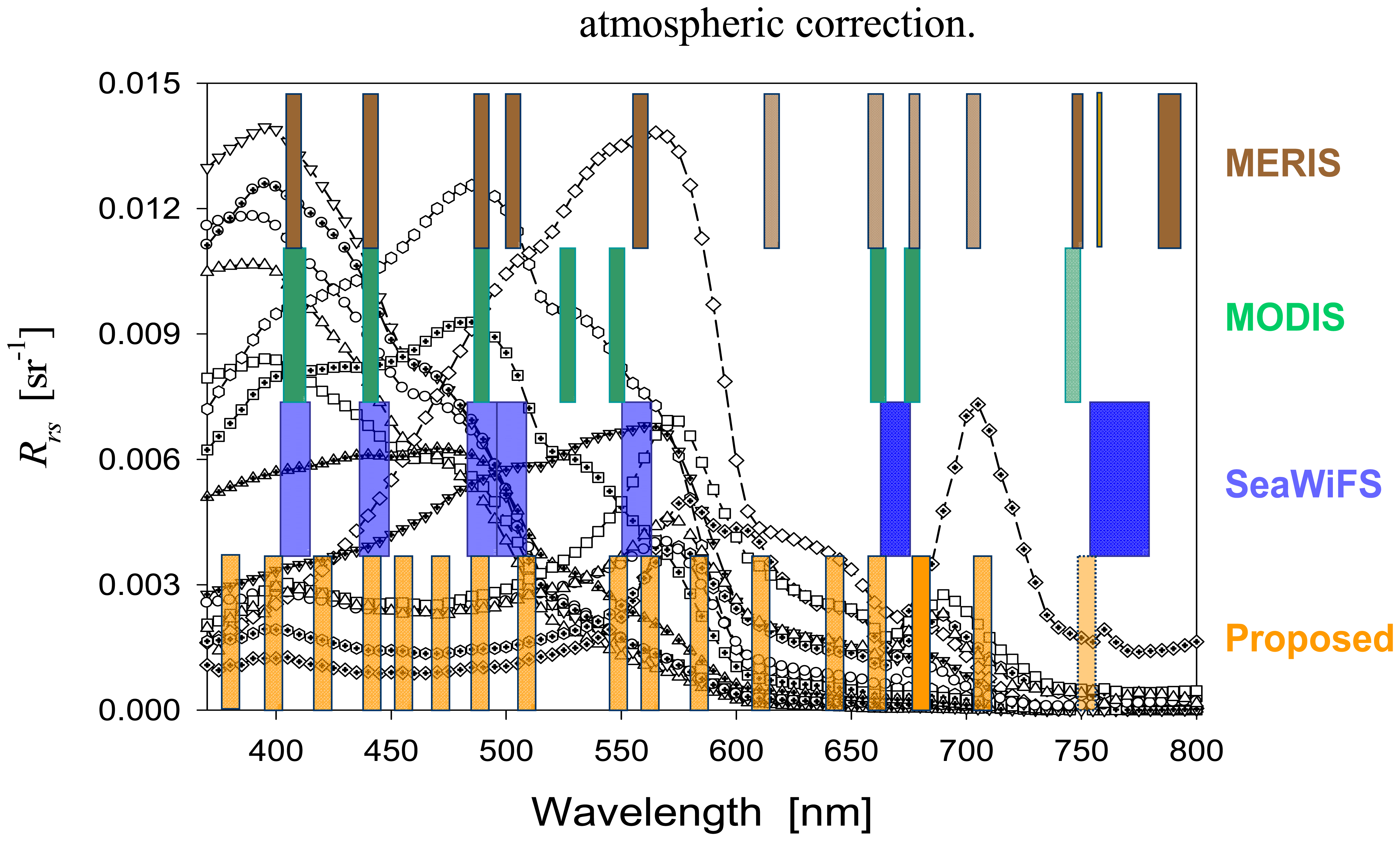
Ideally, to maximize the potential of observing properties of aquatic environments and their temporal and spatial changes, it is best to have a sensor capable of collecting signals with a continuous spectrum. After consideration of data flow, processing, and storage as well as signal-to-noise ratios, satellite sensors commonly have a few bands in the visible and near-IR domain (IOCCG 1998). For instance, the CZCS had five bands, while SeaWiFS and MODIS have seven (or eight) bands (with slightly different configurations). To show the spectral coverage of these operational satellite sensors, Figure 1 presents examples of remote-sensing reflectance spectra, along with the overlaid spectral bands (location and width) of CZCS, SeaWiFS, MODIS, and MERIS. Clearly, for the widely varying reflectance spectra, MERIS collects more spectral information, whereas MODIS and SeaWiFS could miss some important spectral signatures (such as the peak at ∼709 nm and information between 560 – 650 nm), and that CZCS could not observe the reflectance peak at ∼480 nm and the reflectance variation in the blue wavelengths (Carder et al. 1989).
Selection and positioning of those spectral bands were based on measurements and optical characteristics (both absorption and scattering) of phytoplankton and colored dissolved organic matter (IOCCG 1998). 30 years ago, from 31 measurements of spectral reflectance for waters off the Oregon coast, Mueller (1976) demonstrated that reflectance spectra could be reconstructed with four principal vectors, suggesting that there are only four major variables for reflectance, and thus implying a requirement of 4 bands or so for an ocean color sensor. Similarly, for measurements made in the New York Bight region and also based on principal component analysis, Sathyendranath et al. (1994) concluded that a sensor with 5 bands (413.5, 447, 515, 560, 638.5 nm) can be as effective as 32 bands for the derivation of chlorophyll concentration. Mueller, however, cautiously pointed out that such conclusions are sensitive to the data sets used for the study. For instance, Dekker et al. (1992) indicated that 9 bands in the 500 – 800 nm range are needed to adequately cover the spectral curvatures of inland waters, and Wernand et al (1997) suggested another set of 5 bands (412, 492, 556, 620, and 672 nm) to re-construct hyperspectral reflectance for waters off the coasts of Netherlands. More importantly, the statistically-determined principal vectors are not physically intuitive in interpreting the spectral reflectance (Mueller 1976).
In general, the spectral configurations of current operational satellite sensors are designed for monitoring chlorophyll concentrations (index of phytoplankton) and colored dissolved organic matter (CDOM) in the open oceans, but have not been optimized for remote-sensing of complex coastal waters. Lee and Carder (2002) demonstrated that for adequate remote sensing of major properties (water column and bottom) of both open ocean and complex coastal aquatic environments, a sensor requires ∼ 15 spectral bands in the 400 – 800 nm range in order to obtain similar results as a sensor with 81 consecutive bands with 5-nm spacing. It is not yet clear, however, where the 15 bands should be placed.
In this study, from nearly 400 measurements of hyperspectral remote-sensing reflectance from various oceanic and coastal waters, we derived the spectral locations of the optimal bands via first- and second-order derivatives of the remote sensing reflectance for future advanced multi-band sensors for observing properties of aquatic environments. These bands can thus capture most of the spectral variations in remote-sensing reflectance caused by differing water-column and/or bottom properties, and be sufficient to re-construct hyperspectral remote-sensing reflectance spectra if desired.
2. Data and Methods
Since 1993, for a span of more than 12 years, an extensive remote-sensing-reflectance suite of hyperspectral (∼350 – 900 nm with a resolution ∼3 nm) measurements for various aquatic environments was collected, most of which were taken by the Ocean Optics Lab led by Prof. Kendall Carder at the College of Marine Science of the University of South Florida. Table 1 summarizes the cruises and general information of the various environments. The measured waters included open ocean blue waters to turbid coastal yellowish waters and optically shallow waters (bottom depths in a range ∼ 1 – 25 m). Wide ranges of concentrations of chlorophyll and dissolved organic matter and suspended sediments, along with different types of phytoplankton were encountered during these measurements.
Spectral remote-sensing reflectance (Rrs(λ)) is defined as the ratio of water-leaving radiance to downwelling irradiance. The Rrs spectrum contains sub-surface information of water constituents and/or bottom properties (when the bottom is optically shallow). Using a handheld spectroradiometer (Spectron Model SE-590 of Spectron Engineering, Inc. before 1997; SPECTRIX (Steward et al. 1994) for 1997 and later), a series (∼ 3 to 5 scans) of upwelling radiance above the surface (Lu(0+)) and the downwelling sky radiance (Lsky) were directly measured by the instruments for each station of the many cruises. All these measurements were carried out following the NASA protocols described in Mueller et al. (2002).
The measured Lu is a sum of photons emerged from subsurface scattering (the desired signal) plus surface-reflected sky and solar light (noise). Downwelling irradiance was derived by measuring the radiance (LR) reflected from a standard diffuse reflector (Spectralon®). For each of the collected scans, hyperspectral total remote-sensing reflectance (Trs(λ)) and sky reflectance (Srs(λ)) were derived through
with RR the reflectance of the diffuse reflector (Spectralon, ∼ 10%).
Based on these measured Trs and Srs curves, after rejecting obvious outliers, averages of Trs and Srs for each station were obtained, respectively, in order to reduce the random variations associated with the measurements. Further, because Trs is the sum of water-leaving radiance and surface-reflected sky radiance, Rrs(λ) is calculated as (Austin 1974; Carder and Steward 1985)
where F is surface Fresnel reflectance (around 0.023 for the viewing geometry), and Δ accounts for the residual surface contribution (glint, etc.). Figure 2 shows some examples of spectral Trs (Fig. 2a) and Srs (Fig. 2b). Srs spectra are monotonic decreasing functions of λ, whereas Trs spectra, because of the contribution of Rrs, show distinct variations from place to place. In the calculation of Rrs, Δ was determined either by assuming Rrs(750) = 0 (clear oceanic waters) or iteratively derived relative to optical models (coastal turbid waters). Because we are interested in the first- and second-order derivatives of Rrs (see the following for details), inaccurate Δ values have insignificant effects on this study.
Rrs is a function of the total absorption and backscattering coefficients (Gordon et al. 1988; Lee et al. 2004; Zaneveld 1995) as well as bottom reflection (Lee et al. 1998; Maritorena et al. 1994). Spectra of backscattering coefficients, although normally stronger at shorter wavelengths, generally do not have strong spectral signatures (Boss et al. 2004; Loisel and Morel 1998; Twardowski et al. 2001). The spectrum of the total absorption coefficient, however, is a sum of the contributions of CDOM, various pigments contained in phytoplankton, plus water molecules (Gordon and Morel 1983; Smith and Baker 1978; Stramski et al. 2001). These contributions are spectrally selective, and thus result in significant variations in the spectral signatures of the total absorption coefficient (Kirk 1994; Mobley 1994). The extreme values (local maximum or minimum) of Rrs(λ) and the inflections of Rrs(λ) indicate the spectral effects of different combinations of those optically active constituents and/or bottom properties. If a sensor has only a few spectral bands and is intended to best capture the spectral signatures of Rrs(λ), then these bands need to be positioned at wavelengths that can match the locations of those extrema and inflections of Rrs(λ), unless the Rrs(λ) values at those bands are perfectly correlated. The spectral locations for such Rrs(λ) values are those wavelengths with zero first- and second-order derivatives of Rrs(λ), respectively.
To locate the optimal spectral positions for all collected samples, we thus carried out the following calculations:
where σ(λ) and ς(λ) are the first- and second-order derivatives of Rrs(λ), respectively. Note that derivative analysis of hyperspectral data is a widely used tool to highlight and enhance the spectral characteristics in various applications (e.g., Holden and LeDrew 1998; Tsai and Philpot 1998). Before calculating the derivatives, Rrs(λ) spectra were interpolated to 1-nm resolution and were smoothed with a 5-nm running average, in order to remove some of the random noises.
3. Results and Discussions
From all of the calculated σ(λ) and ς(λ) spectra, we obtained the spectral distributions (at 1-nm resolution) where σ(λ) and ς(λ) equal zero, respectively. Mathematically, these frequency distributions are,
Here σi(λ) and ςi(λ) are the ith σ(λ) and ς(λ) spectrum of the data set, respectively. Figures 3 and 4 show fσ(λ) and fς(λ), after a 5-nm running average was applied to highlight the major bands. The frequency distributions of σ(λ) and ς(λ) for wavelengths longer than 700 nm are not considered here, simply because that for oceanic and most coastal waters the Rrs values in those wavelengths are very small due to the strong absorption of water molecules and limited scatters in the water media. Consequently, Rrs in those wavelengths are either non-informative regarding constituents in water, or too noisy in the measured Rrs, except for highly turbid river plume or inland waters or clear and bright-bottom shallow (< ∼1 m) waters.
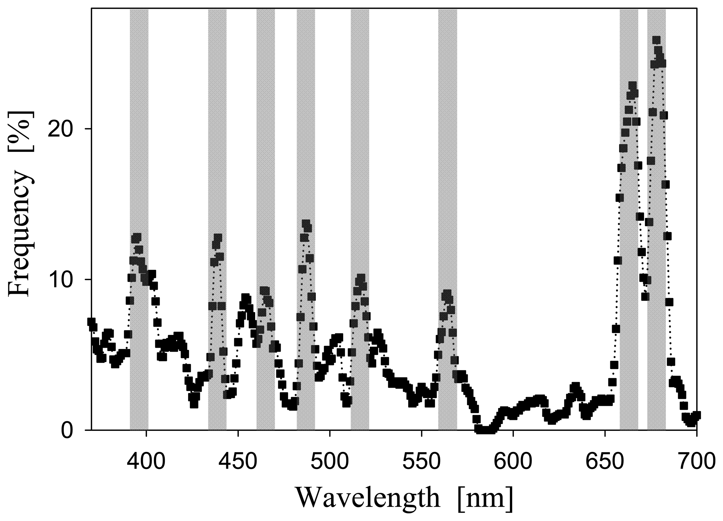
For an Rrs(λ) spectrum, σi(λ) = 0 indicates that there is an extremum of Rrs at λ. For various waters, because of the different combinations of water constituents and/or bottom characteristics, the spectral locations of the extrema shift (see Fig. 1). The spectral distribution of fσ(λ) then summarizes, for all data in this study, the wavelength behavior in capturing the extrema. The greater the fσ(λ) value, the more appearances of an extrema at that λ. Although each wavelength shows some possibility of capturing extrema of Rrs, apparently, the bands that captured more extrema of Rrs are concentrated in seven bands (in the 360 – 700 nm range) instead of spectrally scattered evenly (see Fig. 3). The seven bands are centered at (rounded to nearest 0 or 5): 395, 440, 490, 515, 565, 665, and 685 nm. Such a result is not surprising. For instance, 440 nm is at the peak absorption of phytoplankton pigments (chlorophyll-a), which can result in a local minimum of Rrs(λ); on the other hand, 685 nm is around the peak of chlorophyll fluorescence, which then contributes a local maximum of Rrs(λ) (see Fig. 1). For the other peaks, such as 490 nm or 515 nm, they normally represent locations of Rrs maximum (see Fig. 1 and Fig. 2a), resulted from minimum absorption coefficients at those wavelengths (Kirk 1994; Mobley 1994). Therefore, a multi-band sensor requires at least these bands to adequately capture the extrema of the various Rrs(λ) spectra.
ς(λ) = 0, on the other hand, indicates an inflection of an Rrs(λ) curvature at λ, normally resulting from different combinations of pigments and water molecules, and/or bottom effects when the water is optically shallow. Table 2 summarizes the wavelengths that capture more inflection points of Rrs(λ) curves (also see Fig. 4). In contrast to the distribution of fσ(λ), the peak values of fς(λ) are much less concentrated spectrally. Interestingly, these bands cover the center wavelengths of the major pigments (Table 2) presented in Hoepffner and Sathyendranath (1991). Such a result supports the inclusiveness of the data set used in this study that covers a wide range of water environments, and encompasses various types of phytoplankton classes (resulting in minor changes in Rrs(λ) curvatures because of different pigment absorptions) and optically shallow environments. For a multi-band sensor, it is necessary to have bands that cover these wavelengths if properties other than chlorophyll concentration (such as pigment composition and/or bottom properties) are also desired from remote sensing of water color.
Consolidating the major bands that have greater values of fσ(λ) and fς(λ) (and considering a 10-20 nm bandwidth for satellite sensors), bands that optimally capture extrema and inflections of spectral Rrs are determined (see Table 2 and Fig. 5). These bands form the basis for a multi-band sensor to monitor aquatic environments (including optically shallow waters), although atmospheric absorption and solar Fraunhofer bands require minor adjustments of band positions for satellite sensors to improve global applicability. Interestingly, the analysis from the first- and second-order derivatives indicates 17 bands in the 385 – 800 nm range for the observation of ocean color, which echoes the findings of Lee and Carder (2002). Bands at 710 and 750 nm are added separately, where 710 nm is important for turbid coastal water and water with extreme phytoplankton blooms (red tide) (Dekker et al. 1992; Gower et al. 1999), and 750 nm and other near-infrared channels (e.g., see MODIS channels) are important/required for atmospheric correction (Gordon and Wang 1994) or for highly turbid inland or river plume waters (Dekker et al. 1992).
Table 2 also presents, for comparison, the spectral bands of MODIS and MERIS. Clearly, the wavelength selections of those sensors are in general supported by the results presented here. Comparing MODIS bands with those from this study or those of MERIS, the significant shortfall of MODIS (and SeaWiFS) is a band between 551 and 667 nm. Such a band is of great value for remote sensing of suspended sediments (IOCCG 2006) or remote sensing of optically shallow waters (Lee and Carder 2002). On the other hand, the band at 385 nm could be very useful either for the detection of red tide (Kahru and Mitchell 1998) or for atmospheric correction over coastal waters.
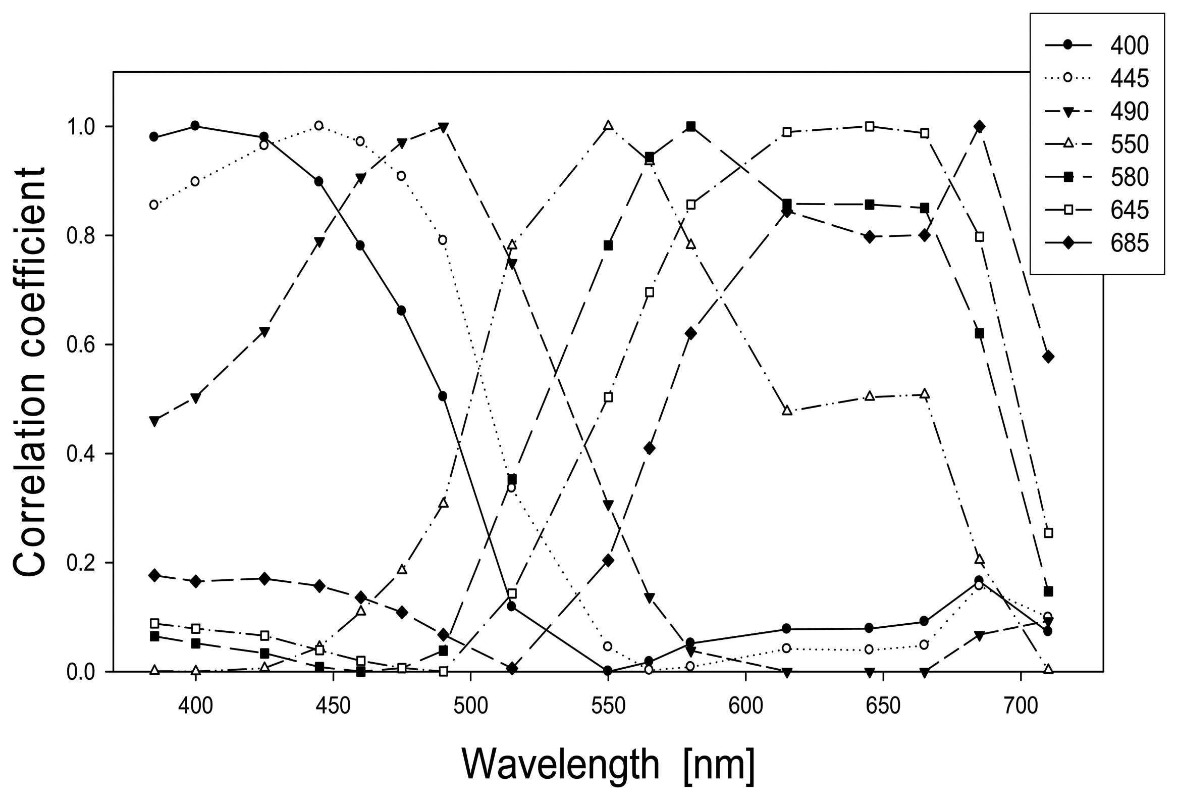
To understand the inter-dependence of Rrs at the selected bands, linear regression analyses of the Rrs at the suggested bands were carried out, and a correlation matrix was obtained. Figure 6 presents a few examples of the correlation spectra. For instance, when Rrs(490) is selected as the independent variable, Rrs at all other bands are considered as dependent, and a correlation spectrum of Rrs is then obtained (Fig. 6). The results from this analysis re-emphasize some known facts: 1) Because the absorption and scattering effects of the individual water constituents are broad-band in nature, the correlation coefficients are high for Rrs(λ) separated by short wavelength distances. 2) Because the absorption coefficients of phytoplankton and CDOM are much stronger in the blue-green region than in the red-infrared region and that they vary independently in general, Rrs in blue-green bands have quite low correlations when compared with Rrs in red-infrared bands (slightly higher correlation for the 670-690 chlorophyll a absorption and fluorescence region). The high correlation coefficients of Rrs at adjacent bands indicate potential redundant measurements when a sensor is exactly equipped with the bands proposed. This is especially true for the bands of 615, 645, and 665 nm where the interdependence is very strong (with correlation coefficients > 0.97). However, as pointed out in the IOCCG Report #1 (1998), “some redundancy is often essential to constrain the solutions”, especially for optically shallow waters where more spectral signal is required in order to adequately separate the information of the water column from that of the bottom. If one band has to be dropped out after considering such high correlation and high overlapping because of 10-20 nm bandwidth of each band, the 645 nm band can be removed from this list. The remaining 615 and 665 nm bands could ensure consistency and continuity with the observations of MODIS and/or MERIS. For waters of Case-1 nature (Morel 1988), however, because the variations of both spectral absorption and backscattering coefficients are determined by chlorophyll concentration alone, Rrs at all wavelengths are correlated (Morel and Maritorena 2001). For such waters and simpler diagnostic requirements, the number of bands can be significantly reduced without losing much information.
4. Summary
In this study, based on extensive and inclusive measurements of hyperspectral remote-sensing reflectance curves from various aquatic environments, the primary bands (in the ∼ 380 – 800 nm range) that optimally capture the spectral signatures of Rrs are determined via first- and second-order derivatives. These bands in general cover the operational bands of SeaWiFS, MODIS and MERIS, and provide important and useful suggestions and guidance for extra bands of future multi-band sensors, in order to provide more and improved results for remote sensing of oceanic and coastal waters. However, these bands are aimed for general observation of the majority (99% or more) of the global aquatic environments and are derived based on available measurements. As point out in Lee and Carder (2002), sensors with discrete spectral bands are always facing the possibility of missing important spectral features of special cases, such as some coral reefs and/or seagrass beds (e.g., Holden and LeDrew 1998). Sensors with higher spectral resolution (along with high spatial resolution) or specially placed bands could be more helpful for such special and challenging cases.
Acknowledgments
We gratefully acknowledge support for this research by NASA Biology and Biogeochemistry Program and NRL 6.2 Project “Lidar and Hyperspectral Remote Sensing” and by the Cooperative Institute for Oceanographic Satellite Studies, which is supported by NOAA award NA03NES4400001. We are also in debt to Thomas Peacock, Jennifer Cannizzaro, Wesley Goode, Liping Li and many others who helped with the collection of such an extensive data set.
References and Notes
- Austin, R. W. Inherent spectral radiance signatures of the ocean surface Ocean Color Analysis SIO Ref.7410. 1974.
- Boss, E.; Pegau, W. S.; Lee, M.; Twardowski, M. J.; Shybanov, E.; Korotaev, G.; Baratange, F. Particulate backscattering ratio at LEO 15 and its use to study particle composition and distribution. J. Geophys. Res. 2004, 109(C01014). [Google Scholar] [CrossRef]
- Carder, K. L.; Steward, R. G. A remote-sensing reflectance model of a red tide dinoflagellate off West Florida. Limnol. Oceanogr. 1985, 30, 286–298. [Google Scholar]
- Carder, K. L.; Steward, R. G.; Harvey, G. R.; Ortner, P. B. Marine humic and fulvic acids: their effects on remote sensing of ocean chlorophyll. Limnol. Oceanogr. 1989, 34, 68–81. [Google Scholar]
- Dekker, A. G.; Malthus, T. J.; Wijnen, M. M.; Seyhan, E. The effect of spectral bandwidth and positioning on the spectral signature analysis of inland waters. Remote Sens. Environ. 1992, 41, 211–225. [Google Scholar]
- Gordon, H. R.; Clark, D. K.; Brown, J. W.; Brown, O. B.; Evans, R. H.; Broenkow, W. W. Phytoplankton pigment concentrations in the Middle Atlantic Bight: Comparison of ship determinations and CZCS estimates. Applied Optics 1983, 22, 20–36. [Google Scholar]
- Gordon, H. R.; Morel, A. Remote assessment of ocean color for interpretation of satellite visible imagery: A review; Springer-Verlag: New York, 1983; p. 44 pp. [Google Scholar]
- Gordon, H. R.; Brown, O. B.; Evans, R. H.; Brown, J. W.; Smith, R. C.; Baker, K. S.; Clark, D. K. A semianalytic radiance model of ocean color. J. Geophys. Res. 1988, 93(10). [Google Scholar]
- Gordon, H. R.; Wang, M. Retrieval of water-leaving radiance and aerosol optical thickness over oceans with SeaWiFS: A preliminary algorithm. Applied Optics 1994, 33, 443–452. [Google Scholar]
- Gower, J. F. R.; Doerffer, R.; Borstad, G. A. Interpretation of the 685 nm peak in water-leaving radiance spectra in terms of fluorescence, absorption and scattering, and its observation by MERIS. Int. J. Remote Sensing 1999, 20(9), 1771–1786. [Google Scholar]
- Hoepffner, N.; Sathyendranath, S. Effect of pigment composition on absorption properties of phytoplankton. Mar. Ecol. Prog. Ser. 1991, 73, 11–23. [Google Scholar]
- Holden, H.; LeDrew, E. Spectral discrimination of healthy and non-healthy corals based on cluster analysis, principal components analysis, and derivative spectroscopy. Remote Sens. Environ. 1998, 65, 217–224. [Google Scholar]
- IOCCG. Minimum requirements for an operational ocean-color sensor for the open ocean.; Morel, A., Ed.; Reports of the International Ocean-Color Coordinating Group, No. 1; p. p. 46. IOCCG: Halifax, Canada, 1998. [Google Scholar]
- IOCCG. Remote Sensing of Inherent Optical Properties: Fundamentals, Tests of Algorithms, and Applications.; Reports of the International Ocean-Colour Coordinating Group, No. 5; Lee, Z.-P., Ed.; IOCCG, Dartmouth: Canada, 2006. [Google Scholar]
- Kahru, M.; Mitchell, B. G. Spectral reflectance and absorption of a massive red tide off southern California. J. Geophys. Res. 1998, 103(C10), 21,601–621,609. [Google Scholar]
- Kirk, J. T. O. Light & Photosynthesis in Aquatic Ecosystems; University Press: Cambridge, 1994. [Google Scholar]
- Lee, Z. P.; Carder, K. L.; Mobley, C. D.; Steward, R. G.; Patch, J. S. Hyperspectral remote sensing for shallow waters. 1. A semianalytical model. Applied Optics 1998, 37, 6329–6338. [Google Scholar]
- Lee, Z. P.; Carder, K. L. Effect of spectral band numbers on the retrieval of water column and bottom properties from ocean color data. Applied Optics 2002, 41, 2191–2201. [Google Scholar]
- Lee, Z. P.; Carder, K. L.; Du, K. P. Effects of molecular and particle scatterings on model parameters for remote-sensing reflectance. Applied Optics 2004, 43, 4957–4964. [Google Scholar]
- Loisel, H.; Morel, A. Light scattering and chlorophyll concentration in Case 1 waters: A reexamination. Limnol. Oceanogr. 1998, 43, 847–858. [Google Scholar]
- Maritorena, S.; Morel, A.; Gentili, B. Diffuse reflectance of oceanic shallow waters: influence of water depth and bottom albedo. Limnol. Oceanogr. 1994, 39, 1689–1703. [Google Scholar]
- Mobley, C. D. Light and Water: radiative transfer in natural waters; Academic Press: New York, 1994. [Google Scholar]
- Morel, A. Optical modeling of the upper ocean in relation to its biogenous matter content (Case I waters). J. Geophys. Res. 1988, 93, 10749–10768. [Google Scholar]
- Morel, A.; Maritorena, S. Bio-optical properties of oceanic waters: A reappraisal. J. Geophys. Res. 2001, 106, 7163–7180. [Google Scholar]
- Mueller, J. L. Ocean color spectra measured off the Oregon coast: characteristic vectors. Applied Optics 1976, 15, 394–402. [Google Scholar]
- Mueller, J. L.; Davis, C.; Arnone, R.; Frouin, R.; Carder, K. L.; Lee, Z. P.; Steward, R. G.; Hooker, S.; Mobley, C. D. Above-water radiance and remote sensing reflectance measurement and analysis protocols; in Ocean Optics Protocols for Satellite Ocean Color Sensor Validation, Revision 3; NASA/TM-2002-210004; Mueller, J. L., Fargion, G. S., Eds.; 2002; pp. 171–182. [Google Scholar]
- Sathyendranath, S.; Hoge, F. E.; Platt, T.; Swift, R. N. Detection of phytoplankton pigments from ocean color: Improved algorithms. Applied Optics 1994, 33, 1081–1089. [Google Scholar]
- Smith, R. C.; Baker, K. S. The bio-optical state of ocean waters and remote sensing. Limnol. Oceanogr. 1978, 23(2), 247–259. [Google Scholar]
- Steward, R. G.; Carder, K. L.; Peacock, T. G. High resolution in water optical spectrometry using the Submersible Upwelling and Downwelling Spectrometer (SUDS). paper presented at EOS AGU-ASLO, San Diego, CA, February 21-25. 1994.
- Stramski, D.; Bricaud, A.; Morel, A. Modeling the inherent optical properties of the ocean based on the detailed composition of the planktonic community. Applied Optics 2001, 40, 2929–2945. [Google Scholar]
- Tsai, F.; Philpot, W. Derivative analysis of hyperspectral data. Remote Sens. Environ. 1998, 66, 41–51. [Google Scholar]
- Twardowski, M. S.; Boss, E.; Macdonald, J. B.; Pegau, W. S.; Barnard, A. H.; Zaneveld, J. R. V. A model for estimating bulk refractive index from the optical backscattering ratio and the implications for understanding particle composition in case I and case II waters. J. Geophys. Res. 2001, 106(C7), 14,129–114,142. [Google Scholar]
- Wernand, M. R.; Shimwell, S. J.; De Munck, J. C. A simple method of full spectrum reconstruction by a five-band approach for ocean colour applications. Int. J. Remote Sensing 1997, 18(9), 1977–1986. [Google Scholar]
- Zaneveld, J. R. V. A theoretical derivation of the dependence of the remotely sensed reflectance of the ocean on the inherent optical properties. J. Geophys. Res. 1995, 100, 13135–13142. [Google Scholar]
Figure 1.
Examples of measured spectral remote-sensing reflectance (Rrs) used in this study. Overlaid are spectral bands (location and width) of CZCS, SeaWiFS, MODIS, and MERIS.
Figure 1.
Examples of measured spectral remote-sensing reflectance (Rrs) used in this study. Overlaid are spectral bands (location and width) of CZCS, SeaWiFS, MODIS, and MERIS.
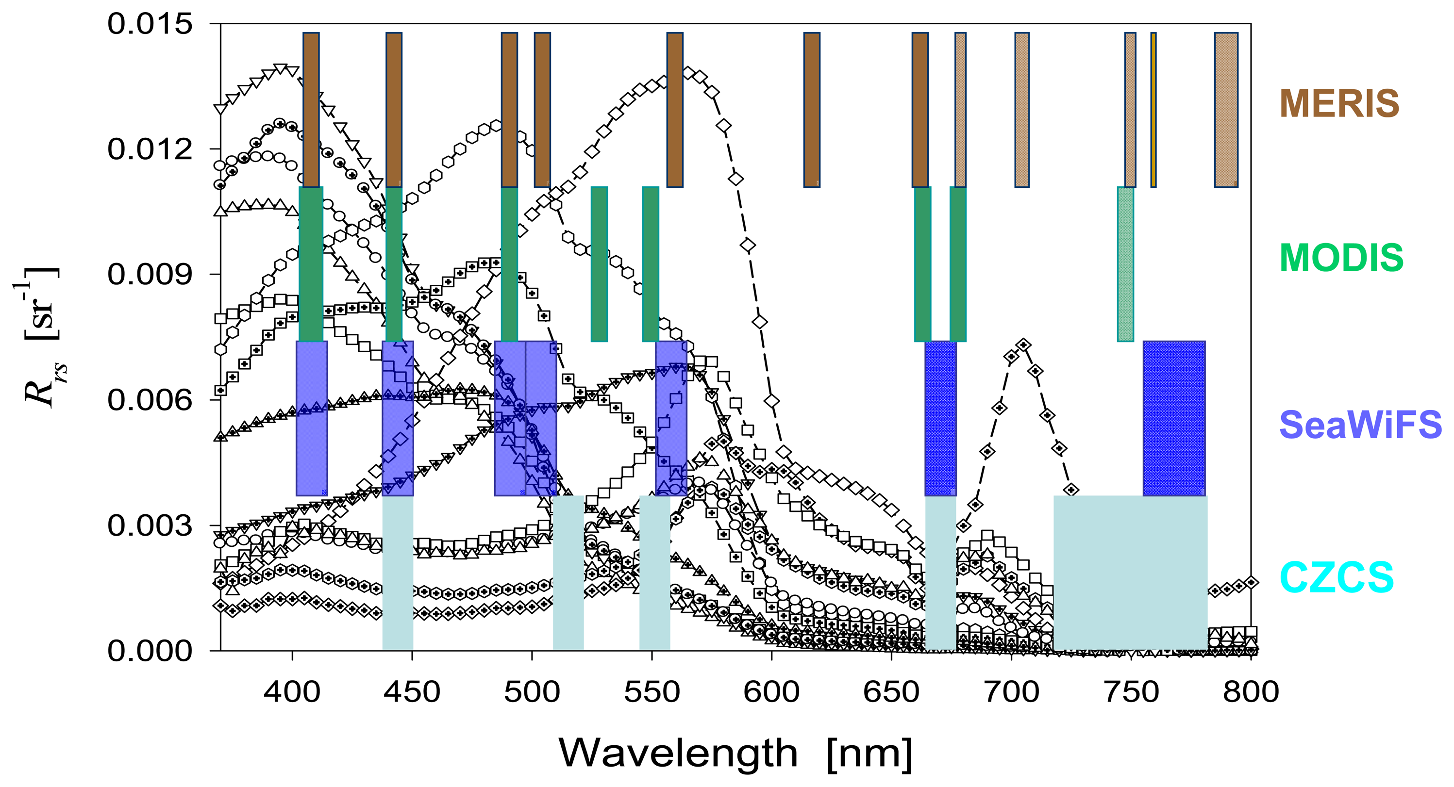
Figure 2.
Examples of spectral total remote-sensing reflectance (Trs, 2a) and sky remote-sensing reflectance (Srs, 2b).
Figure 2.
Examples of spectral total remote-sensing reflectance (Trs, 2a) and sky remote-sensing reflectance (Srs, 2b).
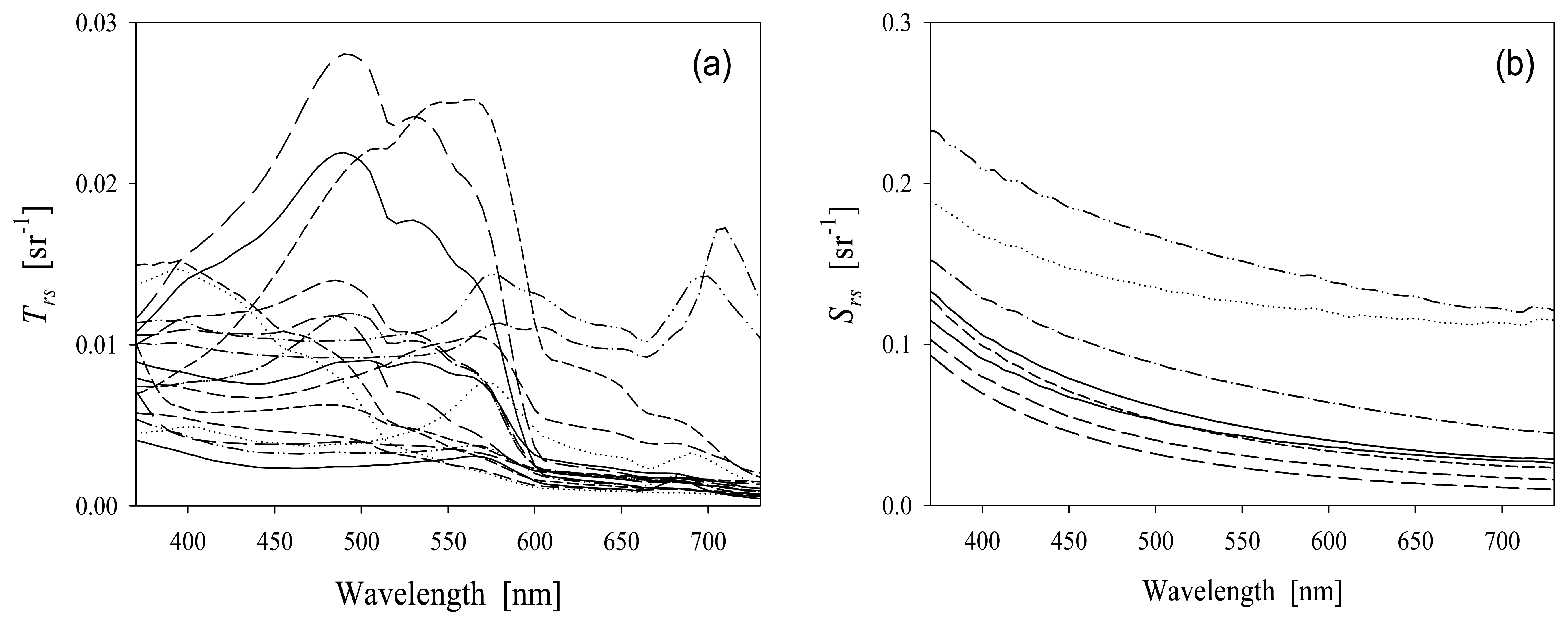
Figure 3.
Spectral distribution of the frequency where the first-order derivative of Rrs(λ) equals 0.
Figure 3.
Spectral distribution of the frequency where the first-order derivative of Rrs(λ) equals 0.

Figure 4.
Spectral distribution of the frequency where the second-order derivative of Rrs(λ) equals 0.
Figure 4.
Spectral distribution of the frequency where the second-order derivative of Rrs(λ) equals 0.
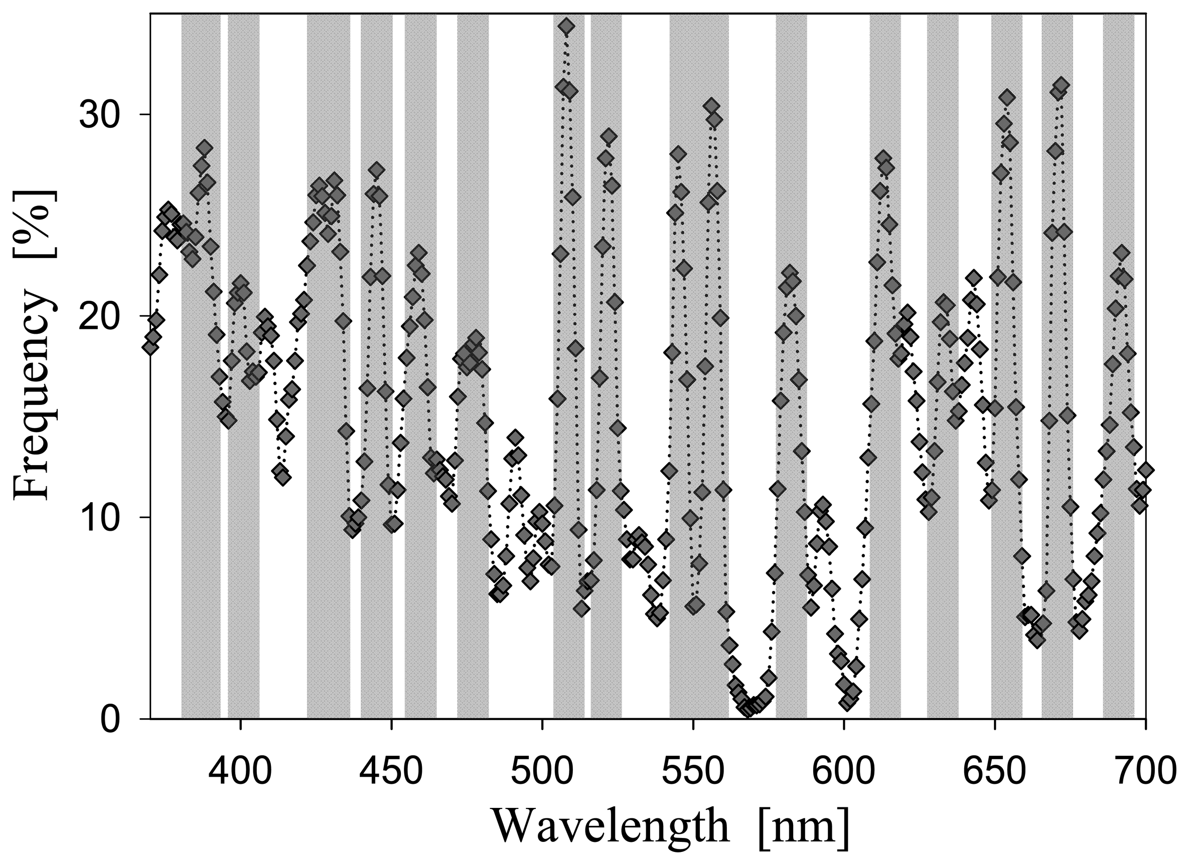
Figure 5.
The spectral bands proposed in this study, overlaid are spectral bands of SeaWiFS, MODIS, and MERIS. The 750-nm band with dotted perimeter indicates that this band is mainly used for atmospheric correction.
Figure 5.
The spectral bands proposed in this study, overlaid are spectral bands of SeaWiFS, MODIS, and MERIS. The 750-nm band with dotted perimeter indicates that this band is mainly used for atmospheric correction.

Figure 6.
Spectral distributions of correlation coefficients of Rrs(λ) at the bands (see Fig. 5) selected from first- and second-order derivative analyses (see text for details). The bands in the insert indicate the Rrs at those bands was used as the independent variable, respectively, while Rrs at other bands were considered as the dependent variable, a correlation coefficient for linear regression was then obtained for each Rrs pair.

| Area | Date | # of measurements | [Chl] range (mg/m3) |
|---|---|---|---|
| Gulf of Mexico | Apr. 1993 | 24 | 0.07 – 49.0 |
| Florida Keys | July 1994 | 5 | 0.06 – 0.5 |
| Arabian Sea | Dec. 1994 | 20 | 0.3 – 0.9 |
| Chesapeake Bay | Sept. 1996 | 36 | 1.7 – 20.7 |
| Hawaii | Feb. 1997 | 6 | 0.1 – 0.3 |
| Florida Keys | May 1997 | 8 | N/A |
| Bahamas | May 1998 | 39 | 0.05 – 1.4 |
| East China Sea | July 1998 | 37 | 0.5 – 2.8 |
| California Coast | Oct. 1999 | 37 | 0.2 – 9.4 |
| North Atlantic | July 2001 | 17 | 4.5 – 13.9 |
| Monterey Bay | Apr. 2003 | 56 | 0.1 – 9.7 |
| Ft. Lauderdale | July 2005 | 52 | N/A |
| Monterey Bay | Sept. 2006 | 47 | 0.5 – 500 |
| Wavelength | Fromfσ(λ) | Fromfς(λ) | Proposed Bands | H&S Bands* | MODIS | MERIS |
|---|---|---|---|---|---|---|
| 385 | x | 1 | 384 | |||
| 395 | x | 2 | ||||
| 400 | x | 413 | 412 | 412 | ||
| 425 | x | 3 | ||||
| 440 | x | 4 | 435 | 443 | 443 | |
| 445 | x | |||||
| 460 | x | 5 | 464 | |||
| 475 | x | 6 | ||||
| 490 | x | 7 | 490 | 488 | 490 | |
| 510 | x | 8 | 510 | |||
| 515 | x | |||||
| 520 | x | 532 | 531 | |||
| 545 | x | 9 | ||||
| 555 | x | 551 | ||||
| 565 | x | 10 | 560 | |||
| 580 | x | 11 | 583 | |||
| 615 | x | 12 | 623 | 620 | ||
| 635 | x | 13 | ||||
| 645 | x | 644 | ||||
| 655 | x | 655 | ||||
| 665 | x | 14 | 667 | 665 | ||
| 670 | x | 676 | ||||
| 685 | x | 15 | 678 | 681 | ||
| 710 | 16 | 709 | ||||
| 750 | For atmosphere correction or turbid river plume water | 17 | 748 | 754 | ||
| 760 | For O2 | 760 | ||||
| 780 | For atmosphere correction | 779 | ||||
© 2007 by MDPI ( http://www.mdpi.org). Reproduction is permitted for noncommercial purposes.
Share and Cite
MDPI and ACS Style
Lee, Z.; Carder, K.; Arnone, R.; He, M. Determination of Primary Spectral Bands for Remote Sensing of Aquatic Environments. Sensors 2007, 7, 3428-3441. https://doi.org/10.3390/s7123428
AMA Style
Lee Z, Carder K, Arnone R, He M. Determination of Primary Spectral Bands for Remote Sensing of Aquatic Environments. Sensors. 2007; 7(12):3428-3441. https://doi.org/10.3390/s7123428
Chicago/Turabian StyleLee, ZhongPing, Kendall Carder, Robert Arnone, and MingXia He. 2007. "Determination of Primary Spectral Bands for Remote Sensing of Aquatic Environments" Sensors 7, no. 12: 3428-3441. https://doi.org/10.3390/s7123428