An Improved Co-evolutionary Particle Swarm Optimization for Wireless Sensor Networks with Dynamic Deployment

State Key Laboratory of Precision Measurement Technology and Instrument, Tsinghua University, Beijing 100084, P. R. China
*
Author to whom correspondence should be addressed.
Sensors 2007, 7(3), 354-370; https://doi.org/10.3390/s7030354
Submission received: 6 March 2007
/
Accepted: 20 March 2007
/
Published: 22 March 2007
Abstract
:The effectiveness of wireless sensor networks (WSNs) depends on the coverage and target detection probability provided by dynamic deployment, which is usually supported by the virtual force (VF) algorithm. However, in the VF algorithm, the virtual force exerted by stationary sensor nodes will hinder the movement of mobile sensor nodes. Particle swarm optimization (PSO) is introduced as another dynamic deployment algorithm, but in this case the computation time required is the big bottleneck. This paper proposes a dynamic deployment algorithm which is named “virtual force directed co-evolutionary particle swarm optimization” (VFCPSO), since this algorithm combines the co-evolutionary particle swarm optimization (CPSO) with the VF algorithm, whereby the CPSO uses multiple swarms to optimize different components of the solution vectors for dynamic deployment cooperatively and the velocity of each particle is updated according to not only the historical local and global optimal solutions, but also the virtual forces of sensor nodes. Simulation results demonstrate that the proposed VFCPSO is competent for dynamic deployment in WSNs and has better performance with respect to computation time and effectiveness than the VF, PSO and VFPSO algorithms.
1. Introduction
Wireless sensor networks (WSNs) has been successfully adopted in many strategic applications such as target tracking, surveillance and classification [1]. Coverage and target detection probability are the two most significant factors for the performance of WSNs [2], which are determined by dynamic deployment algorithms [3]. In initial deployment, randomness is often adopted which, however, always does not lead to effective coverage. Recently, much research effort has been dedicated to dynamic deployment algorithms [3,4,5]. Among these the virtual force (VF) algorithm [6] emerges as one of main approaches for dynamic deployment offering outstanding performance for improving the coverage of WSNs.
Many applications demonstrate that the VF algorithm performs well for self-organizing dynamic deployment [6,7,8]. But these experiments are all implemented in the WSNs consisting only of mobile sensor nodes, but WSNs in practice consist of mobile sensor nodes and stationary sensor nodes to reduce the cost and energy consumption [9]. In this situation, the performance of the VF algorithm will be deteriorated because the force exerted by stationary sensor nodes will hinder the movements of mobile sensor nodes. To solve this problem, Wang [10] proposed a deployment strategy based on parallel particle swarm optimization (PPSO) using the effective coverage performance taken as criterion, where the parallel mechanism is used for saving computation time. However, since the computation complexity of particle swarm optimization (PSO) will increase exponentially as the dimensionality of the search space increases, the computation time is a big bottleneck in PSO.
This paper proposes an improved algorithm, the so-called VFCPSO, combining the VF algorithm with co-evolutionary particle swarm optimization (CPSO) for improving the performance of dynamic deployment optimization. The CPSO algorithm is an improved PSO algorithm inspired by the co-evolution of populations [11], which uses multiple swarms to optimize different components of the solution vectors [12]. In the proposed algorithm, the CPSO is introduced to achieve the dynamic deployment with an improved global searching and regional convergence abilities, while the virtual force is introduced to direct the particles flight to the optimal solutions and enhance the performance of CPSO, i.e., under the guidance of virtual force, CPSO can converge more rapidly and accurately to the optimal results. The organization of the paper is as follows. Section 2 introduces the detection models and a priori assumptions required by dynamic deployment in WSNs. Section 3 introduces the details of the VFCPSO algorithm. Simulation experiments in several typical scenarios have been carried out and are described in Section 4. Finally, Section 5 concludes this paper.
2. Sensor Detection Model and Priori Assumptions
Wireless sensor networks always consist of many stationary sensor nodes and mobile sensor nodes. Because there is no a priori knowledge of terrain or obstacles in the area of interest, all sensor nodes are randomly scattered in the sensing field while initializing. Let us assume that there are K sensors deployed in the random deployment stage, which have the same detection range r. Considering a sensor si deployed at point (xi, yi) , for point P at (x, y) , we denote the Euclidean distance between si and P as d (si ,P). There are two detection models in WSNs: the binary detection model and the probabilistic detection model [6]. Because the detection probability is always uncertain because of the obstacles and noise, the probabilistic detection model is adopted here, which can be present as follows [8]:
where re(re < r) is the measure of uncertainty in detection, λ1 = re -r +d (si ,P) and λ2 = re +r -d (si ,P) ;α1 , α2 , β1 and β2 are the detection probability parameters. It must be noted that this model reflects the behavior of range sensing devices. The values of α1 , α2 , β1 and β2 depend on the characteristics of various types of physical sensors.
In the probabilistic detection model, the detection probability of the sensor field covered by only one sensor node may be less than unity. This means that it is necessary to overlap sensor detection areas in order to compensate for the potential low detection probability in the area which is far from a sensor node. Considering a grid point with coordinates (x, y) lying in the overlap region of a set of sensors Sov , the detection probability of the point that can be successfully detected by at least one sensor node is presented as cx,y (Sov). It can be carried out as follows:
where cx,y (si ) is the detection probability of sensor si at point (x, y) . Then the point ( x, y) can be effectively covered if
where cth is the predefined threshold of coverage probability.
Wireless sensor nodes are always randomly scattered throughout the sensor field. For evaluating the performance of dynamic deployment, the sensor field can be expressed as a two-dimensional grid. The granularity of the grid, i.e. the distance between grid points, can be adjusted to trade off the computation time with the effectiveness. Simulation results verify that the error of the coverage measure is between 0.5% and 0.1% when the granularity is between 4% and 0.25% [10]. During initialization, the area covered by stationary sensor nodes should be analyzed. The points which can be effectively covered by stationary sensor nodes can be ignored during the further analysis to reduce the computation time.
Without loss of generality, we assume that: (1) WSNs consist of a super node which acts as the sink node and processing center for implementing the VFCPSO [13]; (2) mobile sensor nodes can move to the scheduled position exactly; (3) each sensor knows its location by some mechanism such as Global Positioning System (GPS).
3. The Principle of Virtual Force-Directed CPSO
3.1. The Basis of Virtual Force
The virtual force algorithm is a self-organizing algorithm which considers that the objects, including sensor nodes, obstacles and areas of preferential coverage area which need greater certainty [6], will exert virtual attractive and repulsive forces on each other. It is inspired by disk packing theory [14] and the virtual force field concept from robotics [15].
Here, let the total force acted on sensor si be denoted by vector F⃗i , and the force exerted on si by sensor sjbe denoted by F⃗ij . Let F⃗iAm be the attractive force on si due to preferential coverage area Am , and let F⃗iRn be the repulsive force on si due to obstacle Rn . The total force F⃗i on si can be expressed as
where k , M and N are the number of wireless sensor nodes, obstacles and preferential coverage areas.
It's assumed that sensor sj may exert an attractive or repulsive force on sensor si according to the distance dij and a predefined threshold dth:
where C is the communication range,αij is the orientation of a line segment from si to sj , and wA (wR ) is a measure of the attractive (repulsive) force exerted by sensor nodes.
The obstacles will exert repulsive (negative) forces on a sensor. The virtual force of sensor si exerted by obstacle Rn can be presented as follows [8]:
where rRn and pRn are the radius and importance level parameter of the obstacle Rn , wRob is a measure of the repulsive forces exerted by obstacles, diRn is the distance between si and Rn , aiRn is the orientation of a line segment from si to Rn.
The areas of preferential coverage are considered to exert attractive (positive) forces on sensors. The virtual force of sensor si exerted by area of preferential coverage Am can be presented as follows [8]:
where rAm and pAm are the radius and importance level parameter of the area of preferential coverage Am, wApre is a measure of the attractive forces exerted by obstacles, diAm is the distance between si and Am , aiAm is the orientation of a line segment from si to Am.
Then the new location of sensor si is calculated according to the orientation and magnitude of the total force Fxy exerted on it as follows [8]:
where, MaxStep is the predefined single maximum moving distance, Fx, Fy are x- and y-coordinate forces respectively.
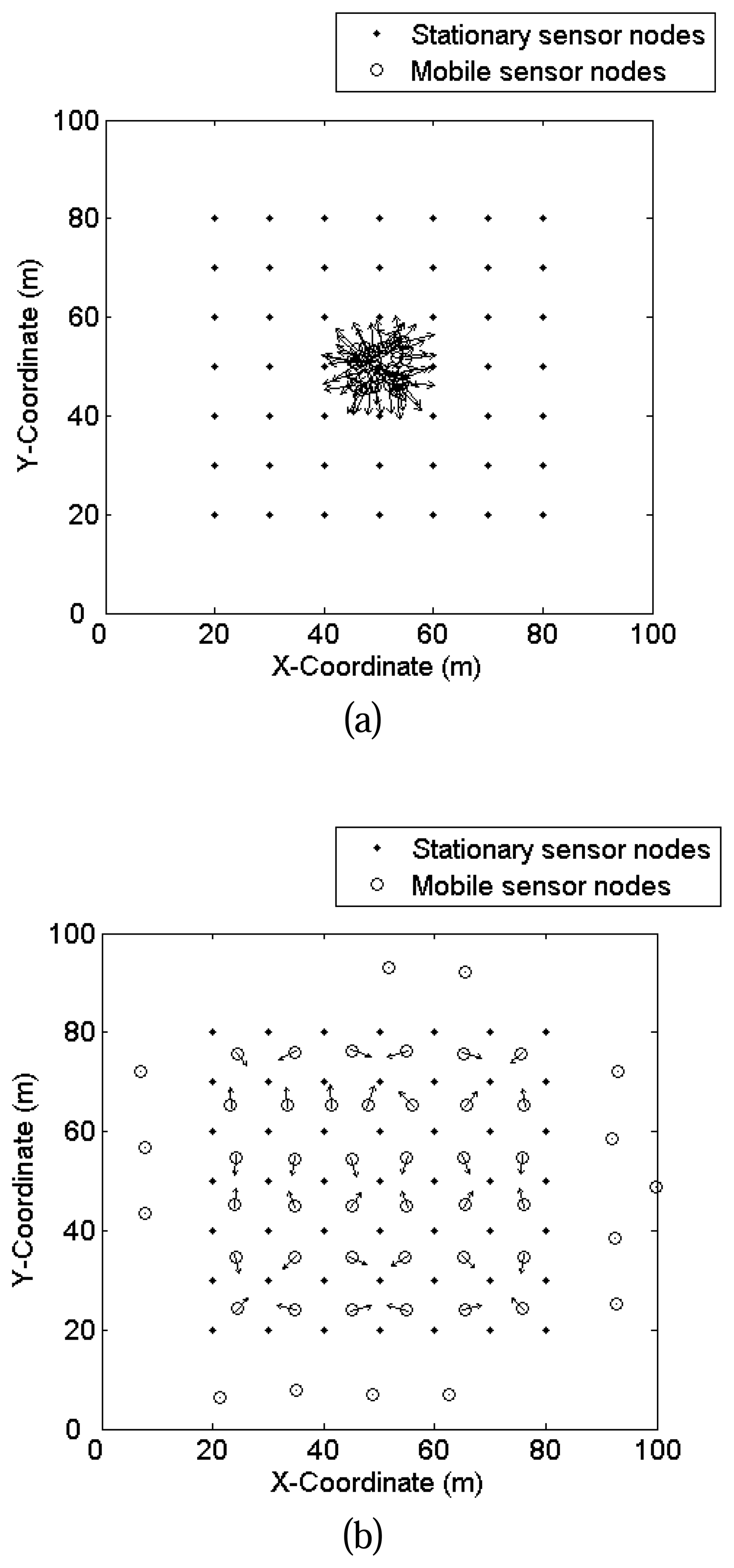
Although the VF algorithm is proven to perform well in WSNs with only mobile sensor nodes [6, 7, 8], its performance may be deteriorated in the context of WSNs with stationary sensor nodes and mobile sensor nodes. Figure 1 illustrates an example of dynamic deployment after 1000 iterations of the VF algorithm, where the arrows present the orientations and magnitudes of virtual forces between wireless sensor nodes. Obviously, most of the mobile sensor nodes are badly confined in the boundary of stationary sensor nodes, which imply that the virtual force exerted by stationary sensor nodes will confine the movement of mobile sensor nodes.
Furthermore, the performance of the VF algorithm largely depends on the threshold distance dth , but it is difficult to find out the proper value of dth because of the various situations and requirements, which are only experientially determined in the current algorithms. Unlike the VF algorithm, the PSO algorithm searches the optimal results globally and will not be impacted by the stationary sensor nodes. Hence, PSO must perform better than the virtual force algorithm in self-adaptiveness and global searching. The details of PSO are introduced in the following section.
3.2. Principle of Dynamic Deployment Based on Virtual Force Directed PSO
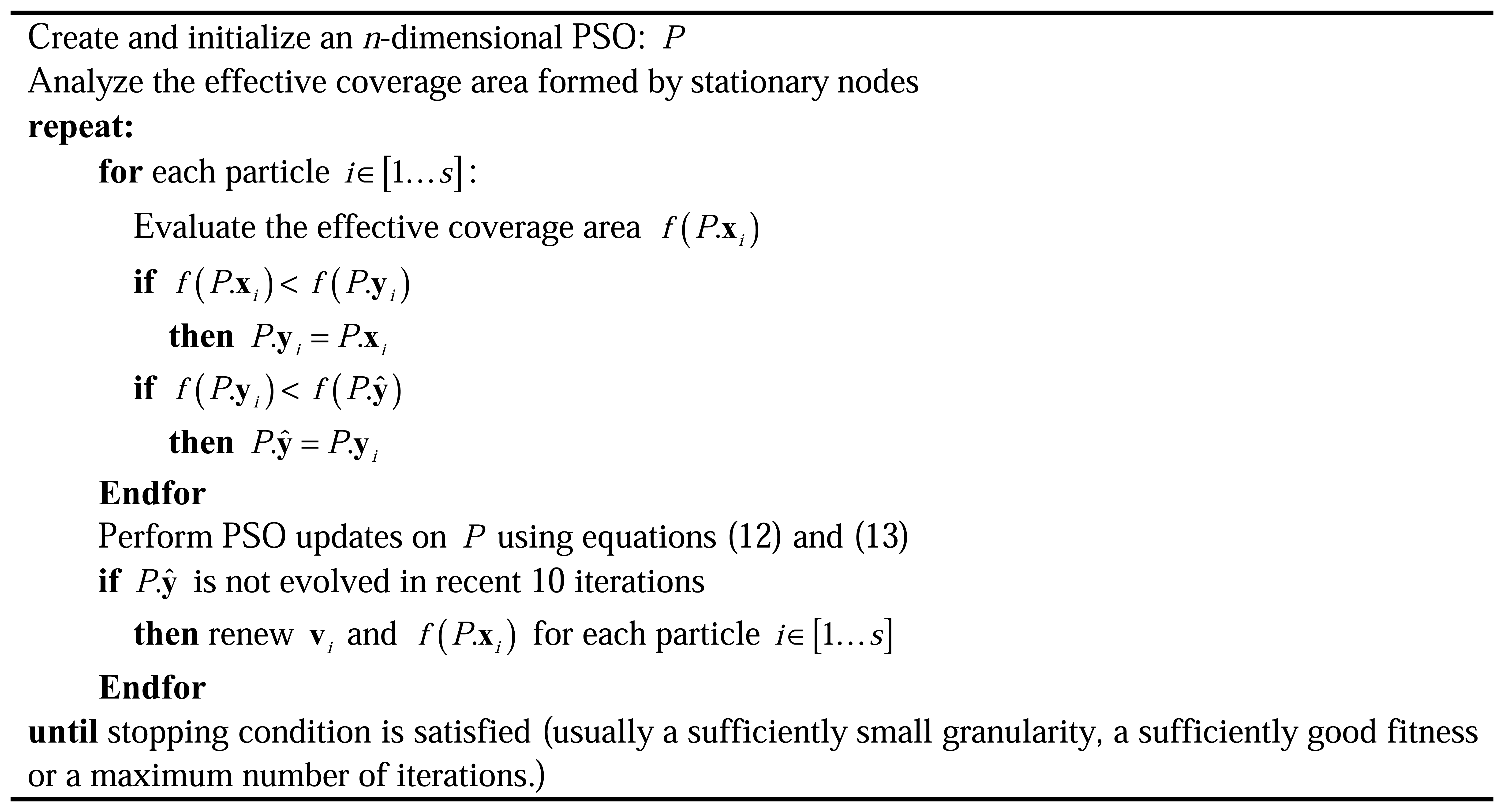
PSO is a swarm-intelligence-based evolutionary algorithm [16]. Each particle represents a potential solution to the optimization task. The particles fly through the search space to find the optimal solution [17]. Let s denote the swarm size. For particle i (1 ≤ i ≤ s) , let yi denote its own local best position, and xi denote its current position. The global best position found by any particle during all previous steps is presented as ŷ . During optimization, each particle updates its current velocity vi toward yi and ŷ with the bounded random acceleration. yi and ŷ are updated as follows:
Then velocity and position of particle are updated as follows:
where c1 and c2 are acceleration constants, r1i (t) and r2i (t) are two separate random functions in the range [0,1], xij (t ) and vij (t ) represent the position and velocity of ith particle in jth dimension at time t, yij (t) is the local best position of ith particle in jth dimension, and ŷ (t) is the global best position. Variable ω(t) is the inertia weight used to balance global and local search, which is always set to
where MaxNumber is the number of maximum iterations.
The elements in the position vector
present coordinates of all mobile nodes, where n is the number of mobile sensor nodes,
presents the x-coordinate of nth mobile sensor node and
presents the y-coordinate of nth mobile sensor node. The fitness of the position vector is presented by the effective coverage area. During global searching, granularity should decrease gradually for the tradeoff between speed and precision. After adjusting granularity, we should renew the velocities of particles randomly and re-analyze the fitness associated with new granularity for keeping the validity. The process of optimization is as follows:
Although PSO is suitable for solving multi-dimensional function optimization in continuous space and the parallel computing mechanism is adopted in [18], the execution time is still a big bottleneck of PSO, especially for large scale wireless sensor networks which consist of lots of mobile sensor nodes.
According to Eq. (12), the velocities of particles are updated according to their corresponding experience and the experience of their companions for pulling each particle toward local best and global best positions in PSO. However, because the initialized positions and velocities of particles are generated by a random term, the convergence speed is partially determined by the initialized parameters of particles. Moreover, the local best and global best positions may not be the optimal results, especially in the forepart of optimization, which will impact the convergence of optimization. Hence, if some other appropriate factors can be introduced to direct the particles flight to the optimal positions, the convergence speed and searching ability of PSO can be improved. It is also the key motivation for importing the virtual force algorithm. Here, an improved PSO algorithm is proposed, the so-called virtual force directed particle swarm optimization (VFPSO), where the virtual force is adopted into the update of velocities of particles for increasing the speed of regional convergence in PSO algorithm.
Different from PSO algorithm, the velocity of each particle is updated according to not only the historical optimal solutions, but also the virtual forces of sensor nodes in the VFPSO algorithm:
where c1 , c2 , r1i (t) , r2i (t) , xij (t) , vij (t) , yij , ŷ (t) , ω(t) are as same as Eq.(15), c3 is acceleration constant, r3i (t) is also a random function in the range [0,1] which is independent to r1i (t) and r2i (t ) , gij (t) is the prolepsis motion suggested by virtual force of ith particle in jth dimension, which is computed by
where the superscript of each parameter presents the index of particles and the index of wireless sensor nodes which the virtual force exerts on, the subscript presents the coordinate of the virtual force. The correlative virtual forces are carried out by Eq. (7). After modifying the velocities of particles with the virtual forces, the VFPSO algorithm also implements the optimization by using PSO according to the flowchart described in the previous section.
3.3. Further Improved VFPSO with Co-evolutionary Manner
Because the traditional PSO algorithm uses a particle to represent a complete solution vector, the search space will be enlarged exponentially as the dimensionality of solution vector. It is significantly harder to find the global optimum of a high-dimensional problem, compared with a low-dimensional problem with similar topology. It will also impact the performance of the VFPSO algorithm. Moreover, the overall evolution of complete solution vector in PSO algorithm has the disadvantage that, during evolution, some components in the vector move closer to the solution, while others may actually move away from the solution. This undesirable behavior is called “two steps forward, one step back” [12].
Co-evolutionary algorithms based on modelling phenomena of coexistence of several species have emerged as a very promising area of evolutionary computing methods [19], such as genetic algorithms [20, 21]. For improving the searching ability of PSO in high-dimensional problem, the search space can be partitioned into lower dimensional subspaces by splitting the solution vectors into smaller vectors [18]. This is the key motivation for co-evolutionary particle swarm optimization (CPSO) [12]. It must be noticed that there is no explicit restriction on the type of PSO algorithm that should be used in the VFPSO algorithm. So, the CPSO can be also used in VFPSO algorithm for improving the performance of dynamic deployment.
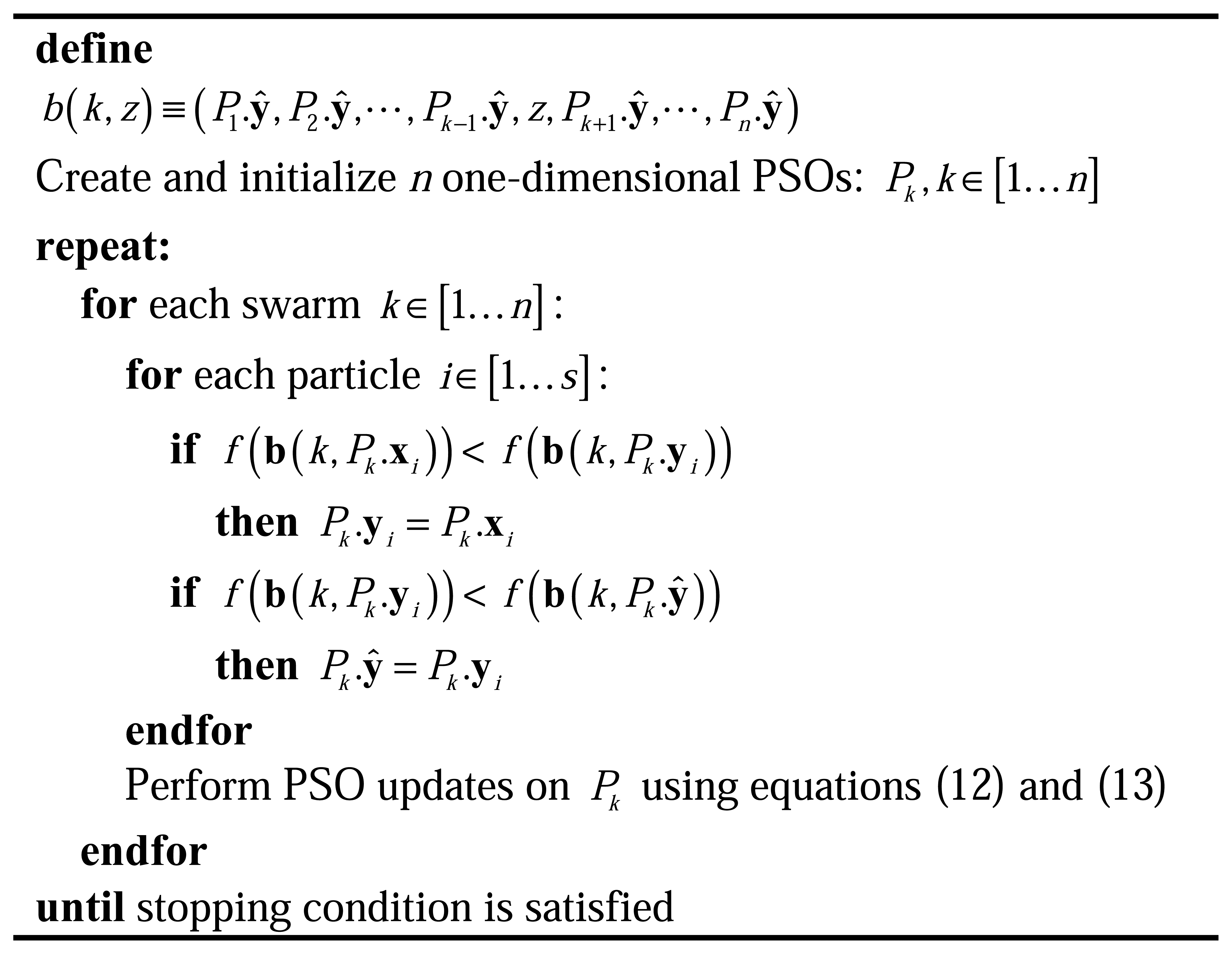
Instead of adopting one swarm to find the optimal n -dimensional vector, in CPSO, the vector is split into its components so that each swarm attempts to optimize a single component of the solution vector, essentially a 1-D optimization problem. However, the function being optimized still requires an n dimensional vector to evaluate. The simplest scheme for constructing such a context vector is to take the global best particle from each of the swarms and concatenate them to form such an n-dimensional vector. To calculate the fitness for all particles in swarm j, the other n-1 components in the context vector are kept constant (with their values set to the global best particles from the other n-1 swarms), while the kth component of the context vector is replaced in turn by each particle from the kth swarm. The pseudocode for the CPSO algorithm is shown in Figure 3, where Pk .xi presents the current position of particle i of swarm k, which can therefore be substituted into the kth component of the context vector when needed, Pk .yi is the local best position of particle i of swarm k and Pk. ŷ is the global best solution of swarm k. The function b(k, z) returns an n-dimensional vector formed by concatenating all the global best vectors across all swarms, except for the kth component, which is replaced with z, where z represents the position of any particle from swarm Pk . Then the current “best” context vector will be denoted b(1,P1.ŷ) , which is composed of the global best particles Pk.ŷ of each of the swarms.
The cooperation between different swarms is promoted by the process of cross-updating in CPSO algorithm. Because the fitness of the context vector is measured when only one component is modified at a time, a significant increase in the solution diversity is advanced in the CPSO algorithm. Although the CPSO algorithm has faster convergent ability, it may become trapped in suboptimal locations in search space [12]. So a hybrid CPSO algorithm is proposed, which can exploit both of these properties. In the hybrid CPSO, an alternative is to interleave the two algorithms, so that the CPSO algorithm is executed for one iteration, followed by one iteration of the PSO algorithm. Then an information exchange between the two algorithms is implemented by replacing some of the particles in one half of the algorithm with the best solution discovered so far by the other half of the algorithm. Because the diversity of particles will decrease significantly because of too-frequent information exchange [12], a simple mechanism to prevent the swarms from accidentally reducing the diversity is implemented by limiting the number of particles that can actively participate in the information exchange.
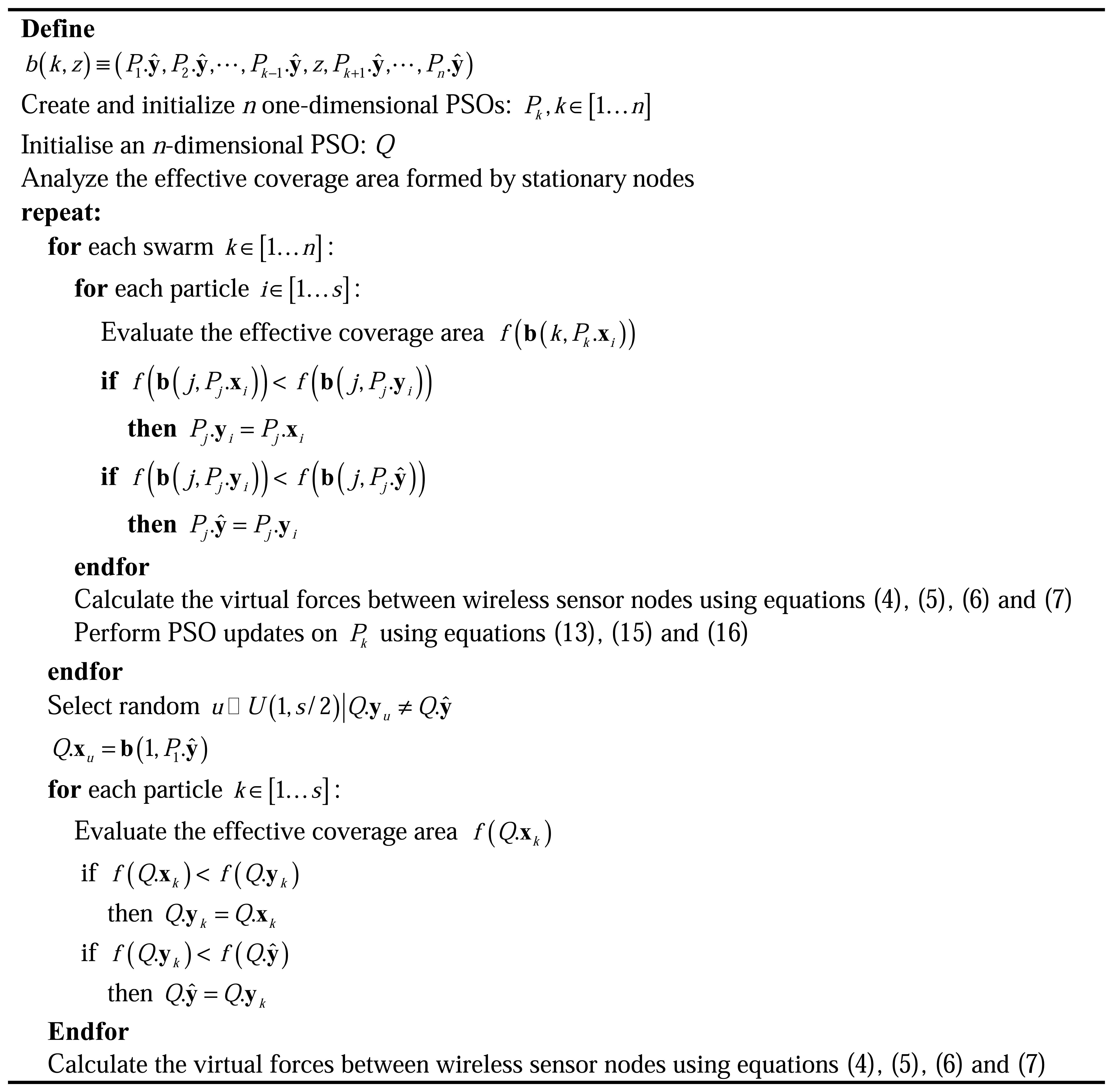
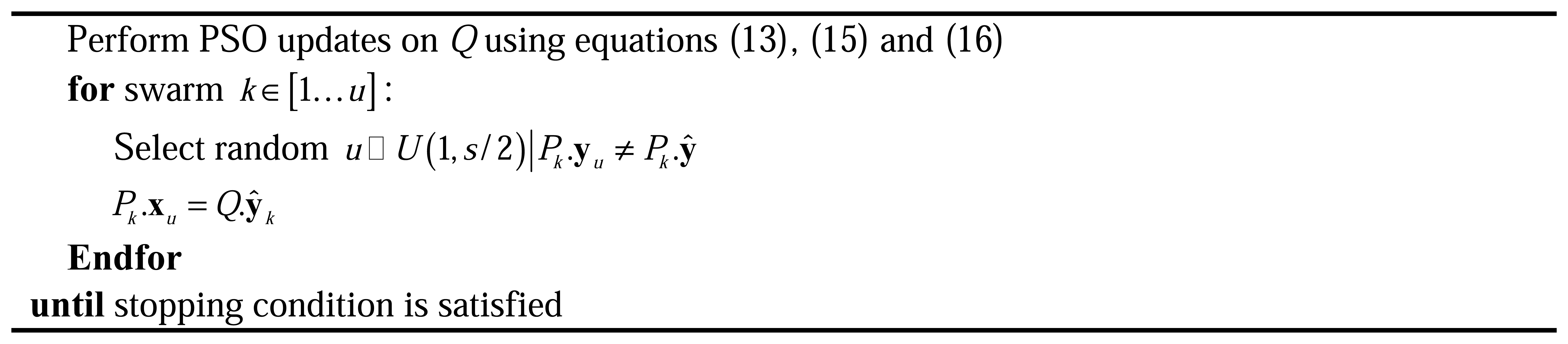
Similar to the VFPSO algorithm, the virtual force directed co-evolutionary particle swarm optimization (VFCPSO) algorithm combines the hybrid CPSO with VF for dynamic deployment in WSNs. In VFCPSO, the global search of optimal deployment is achieved by the hybrid CPSO algorithm in a co-evolutionary manner for improving the solution quality and robustness. The pseudocode for VFCPSO is illustrated in Figure 4, where Q is a normal n-dimensional swarm, Q.xk presents its current position of particle k, Q.yk is the local best position of particle k, Q. ŷ is the global best solution of swarm Q.
Because CPSO can perform better than PSO as the dimensionality of the problem increases [12], the performance of VFCPSO can be improved accordingly. Compared to the VF, PSO and VFPSO algorithms, the VFCPSO algorithm has better global searching and regional convergence abilities and can also be competent for the dynamic deployment of the WSNs with mobile sensor nodes and stationary sensor nodes. The comparisons of the effective coverage area and computation time between VF, PSO and VFPSO and VFCPSO algorithms are carried out in the next section, which verify the outstanding performance of VFCPSO algorithm.
4. Simulation Results
To investigate the performance of the VF, PSO, VFPSO and VFCPSO algorithms in the optimization of dynamic deployment in WSNs, we simulate here different WSN scenarios. VF, PSO, VFPSO and VFCPSO are used to carry out the dynamic deployment respectively. The simulation is done on an AMD Atholon XP1600+ (1.40GHz) PC using MATLAB.
4.1. Comparison of Performance and Computation Time
At first, a WSN including ns = 80 stationary nodes and nm =20 mobile nodes is simulated. The detection radius of each sensor is r = 7m, and the range detection error is re = 0.5r = 3.5m. The sensor nodes are deployed in a square region with area A = 100×100 = 10000m2. The probabilistic detection model parameters are set as α1 = 1, α2 = 0, β1 = 1, β2 = 0.5, cth = 0.9, dth = 2r = 14m, C = 3r = 21m. The parameters for virtual force are set as wA = 1, wR = 5, wRob = 5, wApre =1, MaxStep = 0.5r = 3.5m according to the discussion in [6]. The acceleration constants of PSO are set as c1 = c2 = c3 = 1, MaxNumber = 600 . The numbers of used particles in all PSO algorithms are all 20.
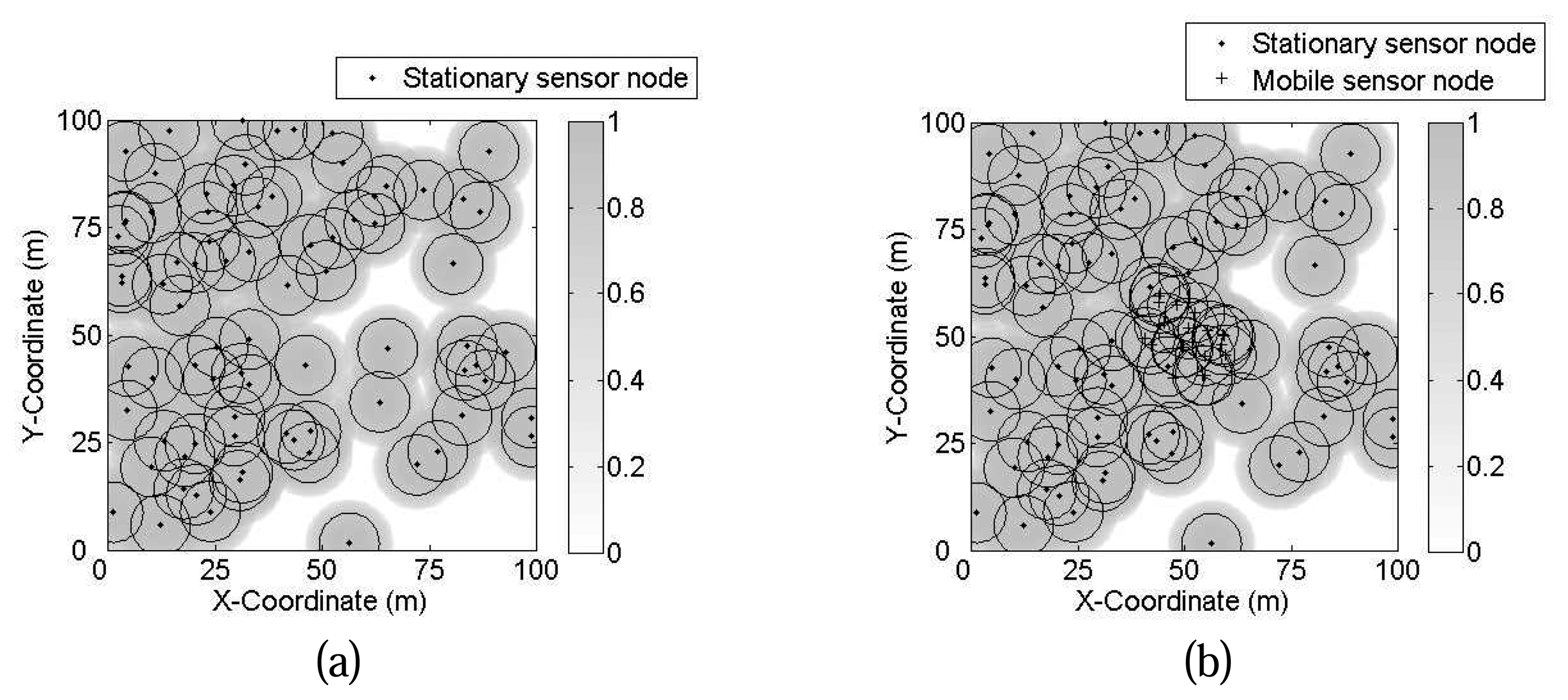
Fig. 5 illustrates the simulation results. The initial locations of stationary sensor nodes are shown in Fig. 5(a), where the effective coverage area is 68.15%. The final results carried out by VF, PSO, VFPSO and VFCPSO are shown in Fig. 5(b), (c), (d) and (e), respectively, where the grey level presents the detection probability of each point. In this independent operate, the effective coverage of the deployment carried out by VF, PSO, VFPSO and VFCPSO are 71.99%, 89.06%, 91.68%, 95.98%.
It is obvious that VFCPSO can implement dynamic deployment most effectively, i.e., the effective coverage area is improved more remarkably than by VF, PSO and VFPSO. The reason is that the co-evolutionary manner significantly increases the solution diversity and improves the robustness and global searching ability of CPSO, and virtual forces of wireless sensor nodes can direct the evolution of particles and increase convergence speed. Furthermore, VF performs worst because the virtual force exerted by stationary sensor nodes impact the optimization of dynamic deployment. PSO cannot achieve the global optimal because the evolution of particles is only suggested by the historical information. Compared to PSO, VFPSO performs better because the combination of virtual force improves the regional convergence ability of PSO. However, the performance of VFPSO is also impacted by the “two steps forward, one step back” scenario.
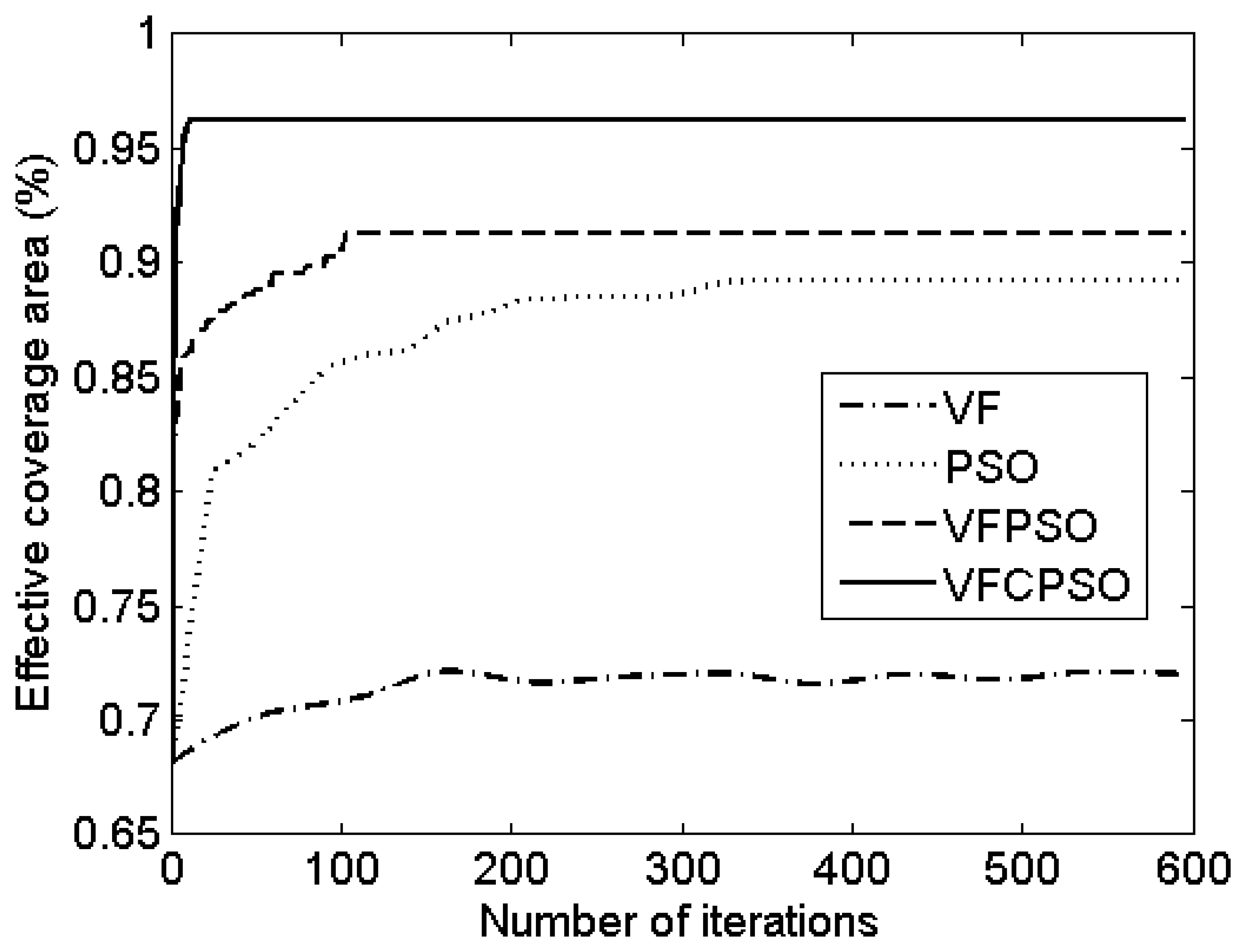
For detailing the comparison of convergence speed, the improvement of effective coverage during the execution of VF, PSO, VFPSO and VFCPSO algorithms in the former individual operation are compared, and the results are shown in Fig. 6. Obviously, VFCPSO can quickly converge to a global optimal with only 12 iterations, while VFPSO is trapped in suboptimal locations in search space with 122 iterations. Without the guidance of virtual force, PSO algorithm improves the effective coverage more slowly than the VFPSO and VFCPSO algorithms, and it also converges to suboptimal after 369 iterations. Furthermore, VF algorithm is significantly impacted by the virtual force exerted by stationary node, so the effective coverage area stays around 71.99% for a long time.
For investigating the robustness of VF, PSO and VFPSO algorithms, 100 independent operations with different initialization are carried out, and the average computation time and mean and mean square root (MSR) of effective coverage area are compared and illustrated in Table 1. It must be noted that the parameters of network and wireless sensor nodes are same in these 100 independent operates.
The results shiw that the dynamic deployment determined by VFCPSO algorithm can effectively cover most area of region of interest (96.36%). And the effect of VFCPSO is also robust since the MSR of effective coverage are of VFCPSO is only 0.54%. The VF algorithm is still impacted by stationary sensor nodes, so the mean of effective coverage area is worse (77.51%). Furthermore, the performance of the VF algorithm is determined by the random initialization of stationary sensor nodes which is not stable, so the MSR of effective coverage area of VF is 7.76%.
Besides the effectiveness and robustness, the VFCPSO algorithm also performs well with regards to computation time. In this scenario, the computation time of the VFCPSO algorithm is less than that of the other three algorithms, implying that VFCPSO is a fast and effective algorithm for dynamic deployment.
4.2. Effect Analyses of the Number of Wireless Sensor Nodes
As presented before, the computation complexity of PSO will increase exponentially as the dimensionality of the search space increases, so the computation time varies significantly relative with the number of wireless sensor nodes in dynamic deployment. For investigating the effect of the number of wireless sensor nodes, a series of experiments in different WSNs which contains different numbers of wireless sensor nodes are implemented. The parameters of different WSNs are listed in Table. 2.
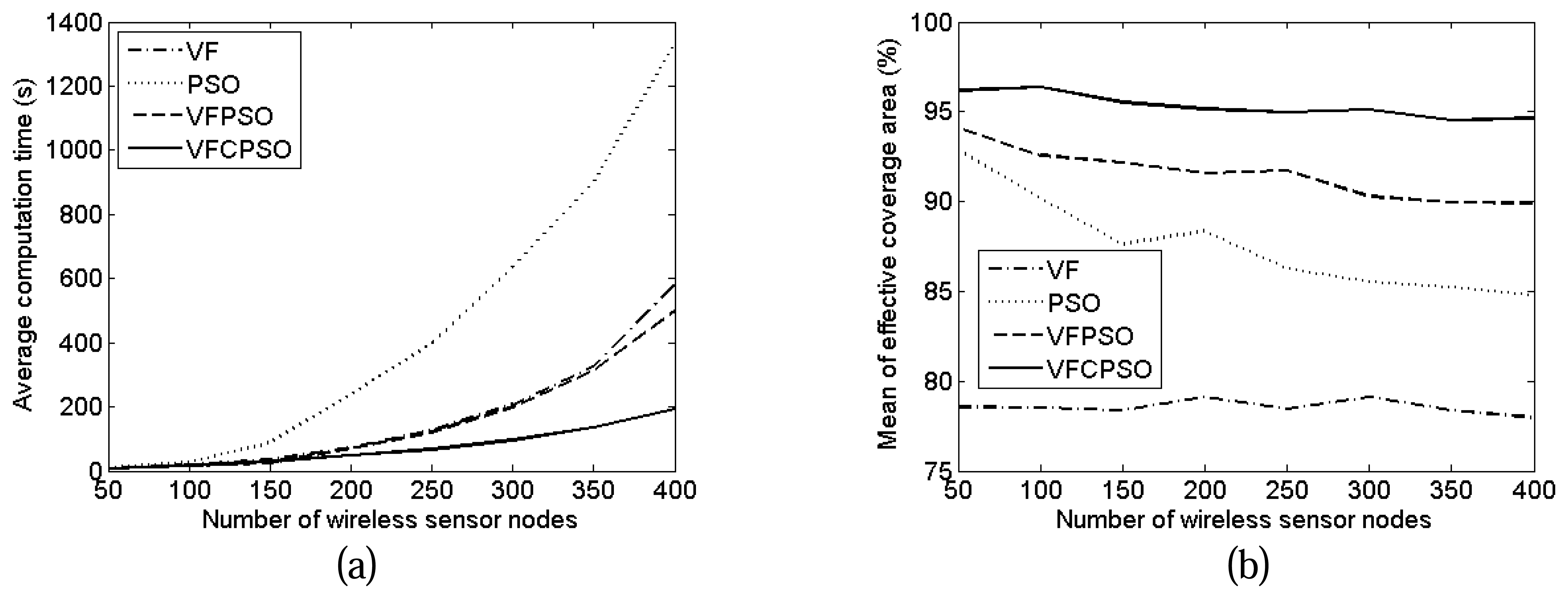
The VF, PSO, VFPSO and VFCPSO algorithms are adopted to deploy the wireless sensor nodes in 100 independent operates for each kind of WSNs respectively. The means of effective coverage area and average computation time of each algorithm in the WSNs which contains different numbers of wireless sensor nodes are illustrated in Fig. 7.
As illustrated in Fig. 7(a), the computation time of four algorithms all increase with the number of wireless sensor nodes. However, the computation time of the VFCPSO algorithm is the least all the time, and its change rate is also the lowest of all four algorithms, which implies that the VFCPSO algorithm can converge to the global optimal most rapidly. Compared to the VFCPSO algorithm, the computation time of the PSO algorithm sharply increases with the number of wireless sensor nodes, because of the exponentially increased computation complexity. The VFPSO algorithm adopts the traditional PSO algorithm, so its computation time also increases faster than the VFCPSO algorithm, although the virtual force can increase its convergence speed. The computation time of the VF algorithm is largely impacted by the complex virtual force exerted on wireless sensor nodes, which is the motivation for its largely increased computation time.
Fig. 7(b) shows that the effective coverage areas of the PSO, VFPSO and VFCPSO algorithms decrease when the number of wireless sensor nodes increases. The reason is that the performance of the PSO algorithms, including PSO, VFPSO and VFCPSO, will deteriorate as the number of wireless sensor nodes increases because the probability of generating a sample inside the optimality region will increase according to the volume of search space. But the performance of VFCPSO deteriorates slower than the PSO and VFPSO algorithms, which implies that VFCPSO has better global optimal search ability and can be adopted in large scale WSNs which contains many wireless sensor nodes. Furthermore, the performance of the VF algorithm is just determined by the randomly initialized dynamic deployment and the parameters of network and wireless sensor nodes, so the effective coverage area of the VF algorithm is irrelative with the number of wireless sensor nodes. However, the performance of the VF algorithm is still worst because it cannot overcome the impact of the virtual force exerted by stationary sensor nodes.
The comparison results of effective coverage area and computation time in different WSNs present the outstanding performance of the VFCPSO algorithm, which demonstrates that this algorithm is a fast, effective and robust algorithm for dynamic deployment in WSNs.
5. Conclusions
This paper proposes an improved co-evolutionary particle swarm optimization algorithm, called the VFCPSO algorithm, as a practical approach for wireless sensor networks with dynamic deployment. In the proposed algorithm, CPSO is adopted to implement global searching of optimal deployment vectors in co-evolutionary manner, virtual force is used to direct the updating of particles towards the better positions. The simulation results illustrate the outstanding performance of VFCPSO algorithm, i.e., VFCPSO is more efficient than the VF, PSO and VFPSO algorithm in terms of effective coverage area and computation time and the performance of the VFCPSO algorithm is nearly stable as the number of wireless sensor nodes increases. It can be declared that the proposed VFCPSO algorithm has good global searching and regional convergence abilities in the procedure of optimization, and it can implement the dynamic deployment of hybrid WSNs with mobile sensor nodes and stationary sensors nodes rapidly, effectively and robustly.
Acknowledgments
This paper is sponsored National Grand Research 973 Program of China (No. 2006CB303000) and National Natural Science Foundation of China (No. 60673176, No.60373014, No. 50175056).
References and Notes
- Chong, C.; Kumar, S. P. Sensor networks: evolution, opportunities, and challenges. Proc. IEEE 2003, 91, 1247–1256. [Google Scholar]
- Wang, X.; Wang, S. Collaborative signal processing for target tracking in distributed wireless sensor networks. J. Parallel Distrib. Comput. 2007. [Google Scholar] [CrossRef]
- Dhillon, S. S.; Chakrabarty, K. Sensor placement for effective coverage and surveillance in distributed sensor networks. Wireless Commun. Network. 2003, 1609–1614. [Google Scholar]
- Qu, Y.-G.; Zhai, Y.-J.; Lin, Z.-T. A novel sensor deployment model in wireless sensor network. J. Beijing Univ. Posts Telecommun. 2004, 27, 1–5. [Google Scholar]
- Heo, N.; Varshney, P. K. A distributed self spreading algorithm for mobile wireless sensor networks. Wireless Commun. Network. 2003, 1597–1602. [Google Scholar]
- Zou, Y.; Chakrabarty, K. Sensor deployment and target localization based on virtual forces. IEEE INFOCOM 2003, 1293–1303. [Google Scholar]
- Wong, T.; Tsuchiya, T.; Kikuno, T. A self-organizing technique for sensor placement in wireless micro-sensor networks. Proc. of the 18th Int. Conf. on Adv. Info. Network. Appl. 2004, 78–83. [Google Scholar]
- Li, S.-J.; Xu, C.-F.; Pan, W.-K.; Pan, Y.-H. Sensor deployment optimization for detecting maneuvering targets. 7th Int. Conf. Inform. Fusion 2005, 1629–1635. [Google Scholar]
- Wang, X.; Ma, J.-J.; Wang, S. Prediction-based dynamic energy management in wireless sensor networks. Sensors 2007, 7, 251–266. [Google Scholar]
- Wang, X.; Wang, S.; Ma, J.-J. Dynamic deployment optimization in wireless sensor networks. Lect. Notes Contol Inform. Sci. 2006, 344, 182–187. [Google Scholar]
- Shi, Y.; Krohling, R.A. Co-evolutionary particle swarm optimization to solve min-max problems. Proc. 2002 Congr. Evolut. Comput. 2002, 1682–1687. [Google Scholar]
- Van den Bergh, F.; Engelbrecht, A.P. A cooperative approach to particle swarm optimization. IEEE Trans. on Evolut. Comput. 2004, 8, 225–239. [Google Scholar]
- Wang, X.; Wang, S.; Ma, J.-J. An improved particle filter for target tracking in sensor system. Sensors 2007, 7, 144–156. [Google Scholar]
- Locateli, M.; Raber, U. Packing equal circles in a square: a deterministic global optimization approach. Discr. Appl. Math. 2002, 122, 139–166. [Google Scholar]
- Howard, A.; Matari′c, M. J.; Sukhatme, G. S. Mobile sensor network deployment using potential field: a distributed scalable solution to the area coverage problem. Proc. of Int. Symp. Distrib. Auton. Robot. Syst. 2002, 299–308. [Google Scholar]
- Ciuprina, G.; Ioan, D.; Munteanu, I. Use of intelligent-particle swarm optimization in electromagnetics. IEEE Trans. Magnet. 2002, 38, 1037–1040. [Google Scholar]
- Eberhart, R. C.; Shi, Y. Particle swarm optimization: developments, applications and resources. Proc. Congr. Evolut. Comput. 2001, 81–86. [Google Scholar]
- Potter, M. A.; De Jong, K. A. A cooperative coevolutionary approach to function optimization. Third Parall. Prob. Solv. Nat. 1994, 249–257. [Google Scholar]
- Danoy, G.; Bouvry, P.; Martins, T. hLCGA: a hybrid competitive coevolutionary genetic algorithm. Proc. Sixth Int. Conf. Hybrid Intell. Syst. 2006, 48–51. [Google Scholar]
- Kim, S. J.; Choi, M.K. Evolutionary algorithms for route selection and rate allocation in multirate multicast networks. Adv. Artif. Intell. 5th Mex. Int. Conf. Artif. Intell. 2006, 426–438. [Google Scholar]
- Schmitt, L. M. Theory of coevolutionary genetic algorithms. Int. Symp. Parall. Distrib. Process. Appl. 2003, 285–293. [Google Scholar]
Figure 1.
An example of VF based dynamic deployment in WSNs: (a) initialization and (b) dynamic deployment result after 1000 iterations, where the arrows present the orientations and magnitudes of virtual forces between wireless sensor nodes.
Figure 1.
An example of VF based dynamic deployment in WSNs: (a) initialization and (b) dynamic deployment result after 1000 iterations, where the arrows present the orientations and magnitudes of virtual forces between wireless sensor nodes.

Figure 2.
Pseudocode for the PSO based dynamic deployment algorithm for WSNs.

Figure 3.
Pseudocode for the CPSO algorithm.

Figure 4.
Pseudocode for VFCPSO algorithm.


Figure 5.
Dynamic deployment after (a) initial random placement and after the optimization of the (b) VF algorithm, (c) PSO, (d) VFPSO, and (e) VFCPSO.
Figure 5.
Dynamic deployment after (a) initial random placement and after the optimization of the (b) VF algorithm, (c) PSO, (d) VFPSO, and (e) VFCPSO.


Figure 6.
The improvement of effective coverage during the execution of the VF, PSO, VFPSO and VFCPSO.
Figure 6.
The improvement of effective coverage during the execution of the VF, PSO, VFPSO and VFCPSO.

Figure 7.
The means of effective coverage area and average computation time of VF, PSO, VFPSO and VFCPSO algorithms in the WSNs which contains different numbers of wireless sensor nodes.
Figure 7.
The means of effective coverage area and average computation time of VF, PSO, VFPSO and VFCPSO algorithms in the WSNs which contains different numbers of wireless sensor nodes.


Table 1.
The average computation time and mean and MSR of effective coverage area of VF, PSO, VFPSO and VFCPSO in 100 independent operations.
| VF | PSO | VFPSO | VFCPSO | |
|---|---|---|---|---|
| Mean of effective coverage area (%) | 77.51 | 90.17 | 92.57 | 96.36 |
| MSR of effective coverage area (%) | 7.76 | 2.45 | 1.13 | 0.54 |
| Average computation time (s) | 19.27 | 27.82 | 17.39 | 15.21 |
| Average iterations | 587.14 | 360.49 | 125.37 | 10.27 |
| Number of mobile sensor nodes | 10 | 20 | 30 | 40 | 50 | 60 | 70 | 80 |
|---|---|---|---|---|---|---|---|---|
| Number of stationary sensor nodes | 40 | 80 | 120 | 160 | 200 | 240 | 280 | 320 |
| Detection radius (m) | 10 | 7 | 5.8 | 5 | 4.5 | 4.1 | 3.8 | 3.5 |
| Range detection error (m) | 5 | 3.5 | 2.9 | 2.5 | 2.75 | 2.05 | 1.9 | 1.75 |
| Communication Range (m) | 30 | 21 | 17.4 | 15 | 13.5 | 12.3 | 11.4 | 10.5 |
| Predefined threshold of virtual force (m) | 20 | 14 | 11.6 | 10 | 9 | 8.2 | 7.6 | 7 |
© 2007 by MDPI ( http://www.mdpi.org). Reproduction is permitted for noncommercial purposes.
Share and Cite
MDPI and ACS Style
Wang, X.; Wang, S.; Ma, J.-J. An Improved Co-evolutionary Particle Swarm Optimization for Wireless Sensor Networks with Dynamic Deployment. Sensors 2007, 7, 354-370. https://doi.org/10.3390/s7030354
AMA Style
Wang X, Wang S, Ma J-J. An Improved Co-evolutionary Particle Swarm Optimization for Wireless Sensor Networks with Dynamic Deployment. Sensors. 2007; 7(3):354-370. https://doi.org/10.3390/s7030354
Chicago/Turabian StyleWang, Xue, Sheng Wang, and Jun-Jie Ma. 2007. "An Improved Co-evolutionary Particle Swarm Optimization for Wireless Sensor Networks with Dynamic Deployment" Sensors 7, no. 3: 354-370. https://doi.org/10.3390/s7030354