Motion Estimation Using the Single-row Superposition-type Planar Compound-like Eye

Department of Mechanical and Electro-Mechanical Engineering, National Sun Yat-Sen University, 70 Lien-hai Rd. Kaohsiung 804, Taiwan
*
Author to whom correspondence should be addressed.
Sensors 2007, 7(7), 1047-1068; https://doi.org/10.3390/s7071047
Submission received: 8 May 2007
/
Accepted: 26 June 2007
/
Published: 27 June 2007
(This article belongs to the Special Issue Intelligent Sensors)
Abstract
:How can the compound eye of insects capture the prey so accurately and quickly? This interesting issue is explored from the perspective of computer vision instead of from the viewpoint of biology. The focus is on performance evaluation of noise immunity for motion recovery using the single-row superposition-type planar compound like eye (SPCE). The SPCE owns a special symmetrical framework with tremendous amount of ommatidia inspired by compound eye of insects. The noise simulates possible ambiguity of image patterns caused by either environmental uncertainty or low resolution of CCD devices. Results of extensive simulations indicate that this special visual configuration provides excellent motion estimation performance regardless of the magnitude of the noise. Even when the noise interference is serious, the SPCE is able to dramatically reduce errors of motion recovery of the ego-translation without any type of filters. In other words, symmetrical, regular, and multiple vision sensing devices of the compound-like eye have statistical averaging advantage to suppress possible noises. This discovery lays the basic foundation in terms of engineering approaches for the secret of the compound eye of insects.
1. Introduction and Motivation
Over one hundred years ago, the configuration of the compound eye of insects started attracting researchers' attentions. Recently, the biologically inspired visual studies have flourished with a boom in the microlens technology. The development of image acquisition systems based on the framework of the compound eye has also progressed quicker than ever. The fabrication of micro compound eye has been reported in the literature with a gradual orientation towards its commercial applications. Those well-known commercial applications include the TOMBO compound eye proposed by Tanita et al. [1], and the hand held plenoptic camera by Ng et al. [2]. The former is a multiple-imaging system with a post-digital processing unit that can provide a compact hardware configuration as well as processing flexibility. The latter is similar to the Adelson and Wang's plenoptic camera [3], but with two fewer lenses, which significantly shortens the optical path and results in a portable device. In addition, some related publications involve one photoreceptor per view direction [4], [5], a miniaturized imaging system [6], the electronic compound eye [7], the curved gradient index lenses [8], an artificial ommatidia [9], and a silicon-based digital retina [10]. All of them belong to the same category of the image acquisition systems with the framework of the compound eye.
Why can the compound eye of insects capture the prey so accurately and quickly? This interesting topic has not been completely answered yet. The biologists believe that it is because of the flicker effect [11]. As an object moves across the visual field, ommatidia are progressively turned on and off. The insects actually measure the distance by the motion of images received by their eyes as they fly [11]–[16]. Because of the resulting “flicker effect”, insects respond far better to moving objects than stationary ones. Honeybees, for example, will visit wind-blown flowers more readily than still ones. Therefore, many researchers have put considerable effort in building images viewed from a compound eye and reconstructing the environmental image from those image patterns [1]–[10]. However, most of those researches are limited to static images. The emphasis of this paper will focus on dynamic vision of the compound eye. In order to achieve motion estimation for visual servo, ego-motion estimation needs to be investigated. Neumann et al. [8] applied plenoptic video geometry to construct motion equations, and optimized the error function to acquire motion parameters. Tisse [10] used polydioptric spherical eyes to develop self-motion estimation. Nevertheless, they employed a more complicated mathematic manner with spherical model. Our paper explains this phenomenon of the insect using a more comprehensive and easy concept with a planar model. The novel characteristics of the compound eye of insects will be examined using a trinocular vision approach. Based on our study on the trinocular vision system [17], it has been shown that incorporating a third camera over traditional binocular, the translational motion can be efficiently resolved. The third camera not only provides more image information, but also significantly improves both efficiency and accuracy for estimation of motion parameters.
2. The Compound-like Eye and Computer Vision
Is there anything special about the image captured by the compound eye? How is the image pattern produced by the compound eye? The mosaic theory of insect vision initially proposed by Muller in 1826, and elaborated by Exner in 1891, is still generally accepted today. According to the mosaic theory, there are two basic types of compound eyes, apposition and superposition [18]. The constructions of these two types are clearly different. The former acquires the image from ommatidium just a small part of overall object, and exploits each ommatidium to make up a complete but ambiguous image; while the latter can acquire a whole image through adjusting ommatidia. Each ommatidium itself receives an ambiguous image, and every image will be different based on its position in the arrangement. Strictly speaking, the terminology of superposition referred here is actually the neural superposition [19], [20].
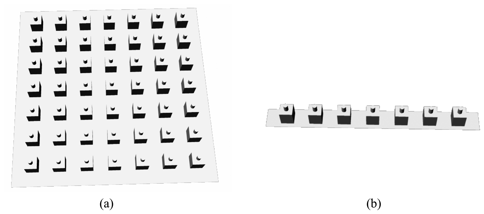
These two types of the compound-eye's structure mentioned above are based on the ecological aspect and can help us realizing how to produce images from compound eyes. But according to the computer vision aspect, which configuration should we adopt to? The compound-like eye used in computer vision proposed by Aloimonos [20] can be divided into two categories. One is the planar compound-like eye, which is a perspective projection module consisting of row and column CCD cameras arranged on a flat plane. Each CCD camera corresponds to an ommatidium of an insect. The schematic diagram is shown in Fig. 1(a). The other is the spherical compound-like eye. The focus of this paper is on a degenerate type of the planar compound-like eye, a single-row planar compound-like eye shown in Fig. 1(b).
How to form the configuration of planar compound-like eye in computer vision? Because generations of images in the superposition and the apposition types are very different, some definitions of compound-like eye in superposition type are described as follows:
- 1)
- Arrangement: Assume each ommatidium is put together in parallel or vertical manner of arrangement in a well-ordered way. Based on this situation, a number of CCD cameras treated as ommatidium are arranged on the surface of a plane. A constant horizontal distance exists between adjacent ommatidia.
- 2)
- Image acquisition: In order to distinguish with the apposition type compound-like eye, the image acquisition of compound eye of insects in superposition type is defined as a whole image through itself ommatidia, so that each ommatidium can look at the whole image of an object.
- 3)
- Image patterns: To produce ambiguous patterns viewed by the compound eye of an insect, assume the image points are deviated from the idea position by possible interfering noises. The contaminated image will result in very different reformed patterns since it is interfered by noises randomly. Therefore the image viewed by each ommatidium will have ambiguous appearances of an object. Besides, each ommatidium creates its image that depends on its different arrangement location. As a result, the images generated by the superposition-type planar compound-like eyes (SPCE) will be close to blurred patterns viewed by ommatidia of an insect.
- 4)
- Simulation: To construct images viewed by the compound eye, the essential pinhole perspective projection will be adopted.
3. Translational Motion for the Parallel Trinocular
Before establishing the translational motion model for the single-row SPCE, the translational motion for trinocular needs to be investigated first. Then, the extension to the translational motion for the single-row SPCE can be made straightforwardly by expanding towards two sides of the parallel trinocular structure.
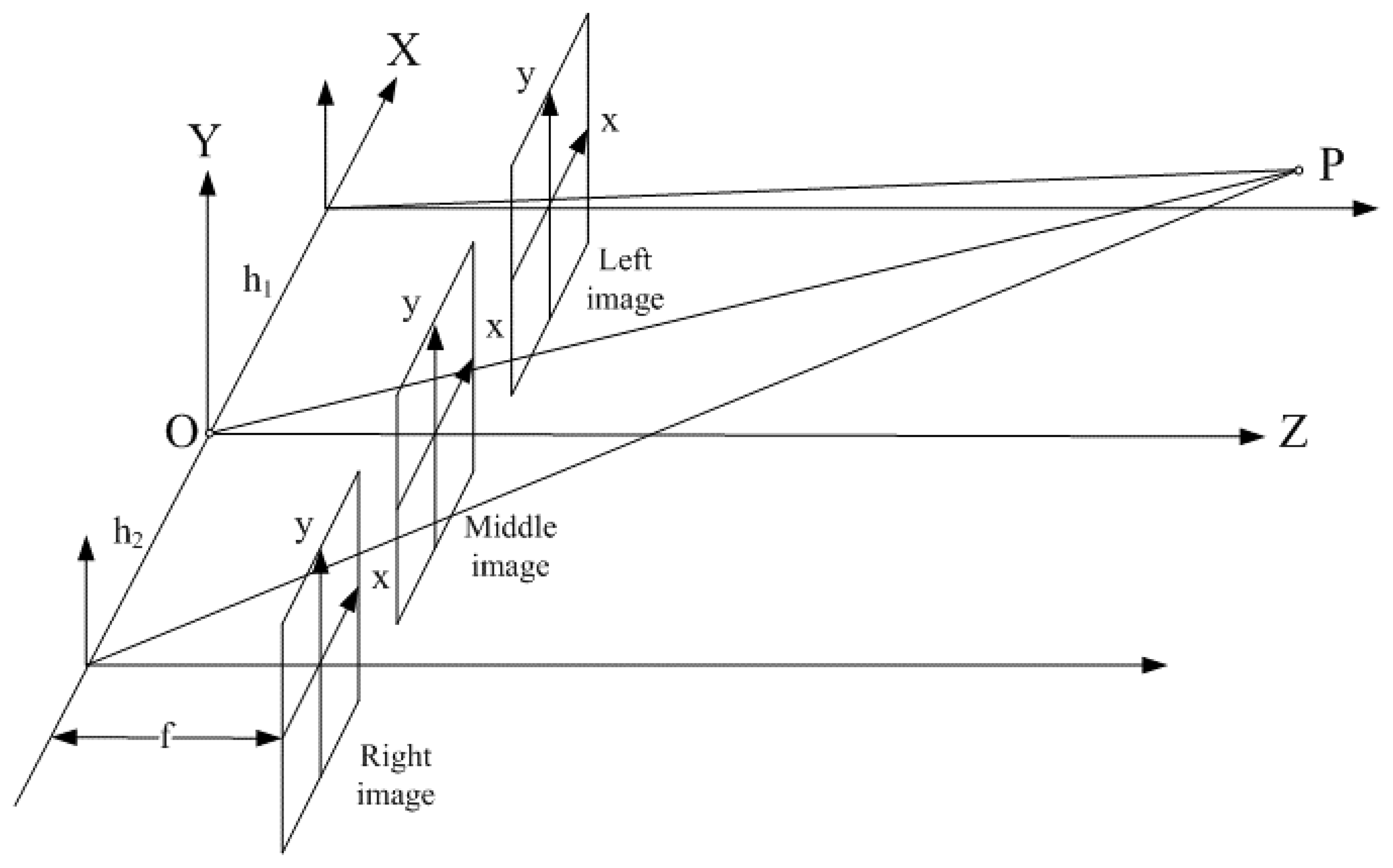
Given O is the origin of a 3D spatial reference frame, assume three identical CCD cameras locating along the X axis and the distances between adjacent cameras are h1 and h2, as illustrated in Fig. 2.
For an arbitrary point P in 3D space, it will project onto the left, middle, and right image planes and the relationships among those three projections can be formulated. Since three cameras are arranged as a parallel trinocular, three images will lie on the same XZ plane. Thus, the y distances for the projections on the image planes will be all the same. However, it is interesting to note that regardless of the distance between adjacent cameras, h1 and h2, the products of the image disparities in X direction meet the following constraint:
where (xl, yl),(xm, ym), and (xr, yr) are corresponding projection points on the left, middle, and right image planes respectively, i and j index two different image points. Please refer to Appendix A for detailed derivation.
Suppose V = (Vx, Vy, Vz)T is the translational motion of the parallel trinocular setup with respect to a moving object. The relations between 2D image velocities, (vix, viy), and the translational motion parameters for each CCD are
where k indexes the left, middle, and right CCDs and has one of those scripts: l, m, and r, f is the focal length, and Z is the depth of the 3-D point.
First select a pair of images that come from left and middle CCDs. The optical flow fields along the X and Y axes for the left and middle CCDs over all pairs of corresponding points can therefore be collected. Because the depths of those two CCDs are the same, they can be easily eliminated. As a result, a pair of image optical flow equations can be derived as follows:
where Ωl and Ωm respectively represent corresponding image regions for the left and middle cameras. The assumption of h1 = h2 = h is also made to simplify further derivation.
The above equations indicate that when the focal length f and the distance h are given, three unknowns for the translational motion if the locations of the image points can be acquired. This configuration implies that using any two CCDs as a set is able to bring about a pair of image optical flow equations. According to this arrangement, increase of the number of CCD brings about the growth of the amount of optical flow equations. If the right and middle CCDs are selected as the second set, and the left and right CCDs as the third set, the above procedure leads to subsequent two pairs of optical flow equations.
For the purpose of simplicity and clarity, the corresponding image regions: Ωl, Ωm, and Ωr are neglected hereafter and some parameters are defined as follows:
Obviously, it is an over-determined problem to solve the translational motion parameters. Due to the special symmetric framework of the arrangement of compound eye, three strategies are applied. Model A includes all optical flow equations. Model B deletes all dependent constraints. Model C keeps the symmetric framework but deletes the relationship between the left and right CCDs.
3.1. Model A (the complete model)
If all equations are considered, then
which can also be formulated in the following matrix expression
The translational motion can therefore be recovered by the standard least square estimation as follows:
Generally speaking, the above derivation can be applied to both point-to-point correspondence and patch-to-patch matching cases.
3.2. Model B (the simplified model)
Much simpler mathematical expressions can be established by getting rid of those equations that are dependent with others. Since Eqs. (3), (5), and (7) are dependent equations, both Eqs. (5) and (7) can be eliminated. Meanwhile, Eq. (6) does not need to be included because it is the sum of Eqs. (2) and (4). Thus, three unknowns can be exactly solved by the following equation:
3.3. Model C (the compromise model)
It just takes time to distinguish equations with dependency. A compromise approach to overcome this difficulty is to ignore the third set of equations that consists of the left and right CCDs with the most dependency by excluding Eqs. (6) and (7). As a result, the matrix expression becomes:
Although the parameters for the translational motion can be resolved by the standard least square approach, possible singularity problem, i.e., the determinant of ATA is zero, still needs to be carefully examined.
The determinant of the matrix ATA for the model C can be obtained as [17]:
It can be shown that (a1b2 − a2b1) ≠ 0 and (a1b3 − a3b1) = 0 (refer to Appendices B, C, and D for detailed derivation). Apparently, the above form is always greater than zero, because the focal length is always positive and the image disparities in the X axis, a1 and b1, are also not zero. Therefore, the singularity problem will not happen in the presented approach. Correspondingly, both Models A and B can also lead to similar results. Appendix E verifies that determinant of matrix ATA for model A is not zero. Similarly, non-zero determinant of ATA for the model B can be easily assured.
Due to the rich relationships among CCDs owned by the parallel trinocular, standard solutions for those three models under the ideal condition of free noise are identical. However, the image will normally be corrupted by noises in real world, and the solutions for the translation will not be similar.
4. Translational Motion for the Single-Row SPCE
Installing more CCDs along two sides of the parallel trinocular gradually reaches a single row SPCE structure. Expanding the image optical flow equations for the translational motion of the parallel trinocular by increasing the number of CCDs also leads to the translational motion model for the single row SPCE. Basically, the approach to solve the single row SPCE is the same as that in the parallel trinocular. The only difference is the orders of the image matrix and the optical flow vector, which should correspond to the amount of CCD.
Assume the amount of CCD at each side from the central camera is q. Then the total number of cameras n in the single row SPCE becomes 2q+1. Therefore, the orders of the image matrix and the optical flow vector for each motion model are summarized in Appendix F. For example, assume the total amount of CCD for a single row SPCE is 7, then the order of the image matrix, optical flow vector for Models A, B, and C will become (42×3, 42×1), (7×3, 7×1), and (12×3, 12×1), respectively. The single row SPCE structure, similar to the parallel trinocular, owns advantages of absence of singularity difficulty and robust solution for motion estimation subject to signal noises, which will be verified by extensive experiments.
Based on the images of SPCE generated from computer vision, recovery of the translational motion using a single-row SPCE can be accomplished by the following procedures:
- 1)
- In order to have the images captured by cameras of the single row SPCE as ambiguous as the picture viewed by ommatidium, random noises are added to ideal images. The fuzziness properties of all individual images are assumed to be independent to one another.
- 2)
- When the single-row SPCE looks at an object, each ommatidium CCD will perceive a different profile according to its given location. In this manner, the compound-like eye will observe a whole picture consisting of many small, similar, and ambiguous patterns.
- 3)
- When the object moves, the single-row SPCE can detect this translational movement using two complete images before and after the motion.
- 4)
- Using those two vague images that include the information of the translation, the corresponding optical flow for each camera can be determined.
- 5)
- Any two CCDs are able to generate a pair of image optical flow equations. The greater the total quantity of the camera is, the more the number of the image optical flow equations becomes.
- 6)
- These large amount of image optical flow equations can be stacked in a matrix form, such as Ax = d, where A denotes the image matrix, d is the optical flow vector, and x is the unknown 3D translational motion.
- 7)
- Using the least square estimation approach, the ego-translational motion can be immediately obtained by x = (ATA) −1ATd.
- 8)
- When the amount of the ommatidium CCD camera grows, the resolved ego-translational motion parameters using the single-row SPCE will approach to the ideal values.
5. Experiments on Motion Estimation
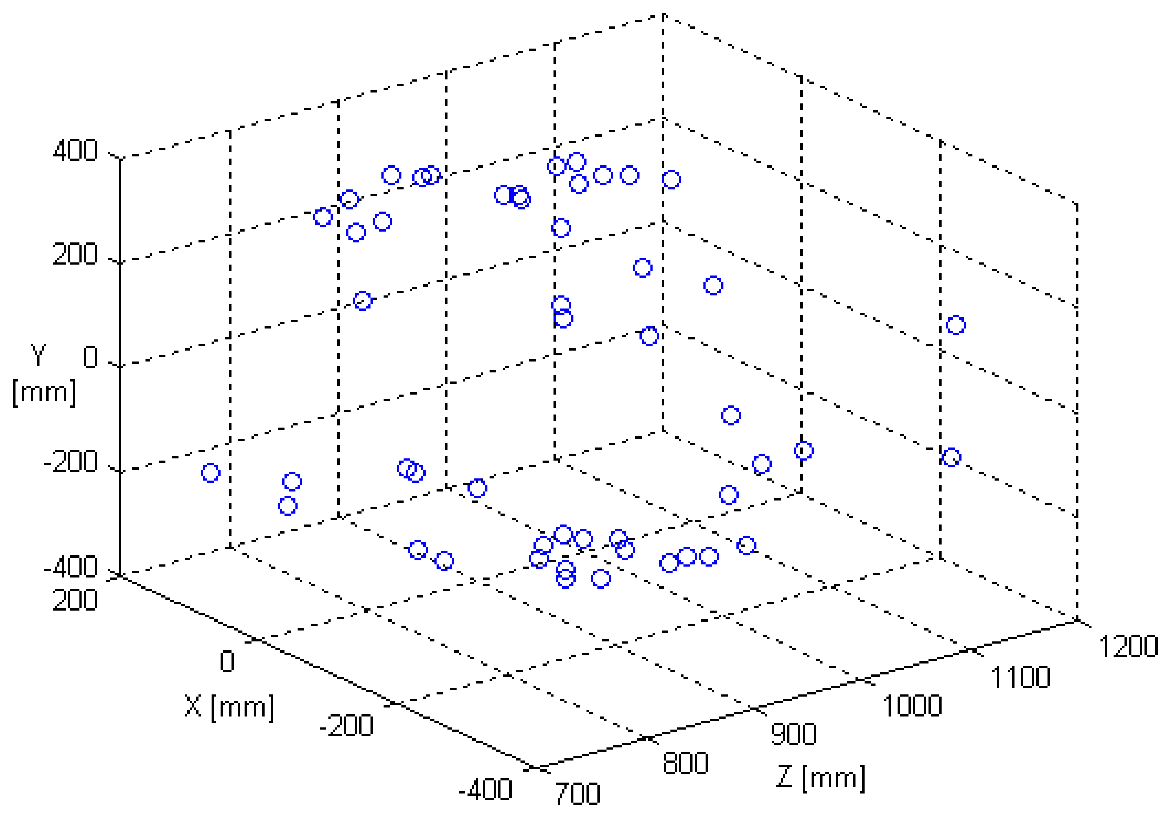
In order to verify the performance of noise immunity for the single row SPCE, a given synthesized cloud of fifty 3D points shown in Fig. 3 is chosen as the test objects in the experiment.
To simulate a realistic situation, noises have to be introduced into ideal data. Gupta and Kanal [23] have tried various noise models, such as uniform noise in a range, Gaussian noise with zero mean and a specified variance, and Gaussian noise with zero mean and a specified fractional variance. Variances of noises in error analysis conducted in [21]–[23] were given proportional to magnitudes of velocity components. The zero-mean Gaussian noise used in this paper is adopted from the works [24], [25]. Their algorithms were validated by incorporating the zero-mean Gaussian noise with simulated realistic data. Garcia and Tziritas [25] further indicated this error model can provide the ability to synthesize errors whose range is similar to that produced by optical flow. Their optical flow noise model was referred by Lobo and Tsotsos [26] as “Gaussian noise with mean 0% and standard deviation b%”. In order to reveal the capability of noise-resistance of the compound-like eye available in large noise environment, a high noise model, which can be described as “Gaussian noise with mean 0 and standard deviation b”, will be employed. The proposed noise model presents 100 times noise level higher than the pre-mentioned one.
Assume the image components in the ideal motion field (x, y) are perturbed by additive zero-mean Gaussian noises. The two noise processes for x and y image planes were independent to each other, and each of them was spatially uncorrelated. For the purpose of reflecting actual implementation in computation of optical flows using image patterns at adjacent time instants, the noises directly occurred on the positions of image pixels and their variances were assumed to be constant over the entire image plane. Therefore, the contaminated image points by the noises before and after a movement were respectively modeled as:
where i indexes the image point, (x(i), y(i)) locates the ideal image point for the i-th point, and N(i) denotes a zero-mean Gaussian random noise at this position. The noise processes Nx1, Ny1, Nx2, and Ny2 are assumed to have the same statistical property and are given by
where σ is the standard deviation. In other words, all image points are contaminated by a random noise with the same variance.
For the purpose of simplification for the follow-up validation and simulation, the translation movement was approximated by the translation velocity under the assumption of unit sampling time. Therefore, the image velocity could imply the image displacement. A small displacement and a large displacement were chosen as (0.1, 0.1, 0.1) and (60, 50, 5) with unit of mm, respectively. According to the above algorithm, for an ideal case free of noise, the estimated ego-translations were correspondingly derived as (0.1, 0.1, 0.1) [mm] and (59.6661, 49.7217, 4.9718) [mm]. Different levels of noise with variance varying from 1 to 100 were studied. Due to movement variation being too small in the small displacement, only the large displacement (60, 50, 5) would be applied for validation. All gap distances between adjacent CCD cameras were 90 mm. The arrangements of CCDs in the single row SPCE include 1×3, 1×5, 1×7, 1×9, 1×11, 1×13, 1×15, and 1×25. A total of 300 trials for each situation were conducted. The image points with different noise variances for the 1×25 single-row SPCE at two contiguous time instants (black and red) are shown in Fig. 4. From Fig. 4, when the level of noise increases, its influence on the image pattern becomes more seriously. And as the variance of noise reaches 16, the profiles for each CCD image were not distinguishable and it is extremely difficult to recognize the corresponding movement.
Considering those ambiguous image patterns contaminated by different levels of noise, model validation based on performance of motion recovery using those three presented motion models will be explored. The relative error is defined as [27]
where (
,
,
) represents the computed translation movement, and (Vx, Vy, Vz) is the actual translation motion.
5.1. Validations of Three Models
5.1.1. Accuracy
For validation of the three Models, additional two cases including an arbitrary single point, i.e., (-365, 112, 960) and any 5 points will be explored. For different single row SPCE configurations under a noise level of variance 100, relative errors of motion recovery in percent of the ego-translation are demonstrated in Fig. 5 for the single point, 5 points, and 50 points in 3D space. The X axis is the CCD camera number of the single row SPCE, the Y axis is the number of test points in 3D space, and the Z axis is the relative error of translation motion. Note that the configuration of the single row SPCE for 1×3 is neglected since the results in those three models are very close.
Based on the experimental results, the following summaries can be made:
- 1)
- Models A and C always keep in the acceptable level when the CCD camera number increases. But Model B cannot converge to a satisfactory level. Since Model A possesses more equations in translation motion estimation, it is not surprisingly less relative errors are found. While Model B owns less equation, the relative error becomes larger. In the single point case, for the 1×155 single row arrangement, it is clear that the relative error of Model A is the best, Model C is next, and Model B is the worst.
- 2)
- It has been shown that the errors decrease quickly when the number of points increases [28]. When the number of test points increases to 50, it appears that the relative error of Model A is not the minimum any more. Considering the case with the 1×155 single row arrangement, the relative error of Model C, 0.46%, becomes better than that of Model A, 0.51%. Nevertheless, Model B is still the worst.
- 3)
- The two relative error curves for Models A and C exhibit interesting variations when the number of test points increases. The intersection point of these two relative error curves are about at 1×29 and 1×70 for the cases of a single point and 5 points, respectively. But when the test point number reaches fifty, it is noted that the intersection point does not exist. This interesting phenomenon clearly indicates the relative error of Model C is close to that of Model A in most situations.
5.1.2. Computational efficiency
Since the dimensions of image matrix and optical flow vector in those three models vary with the CCD camera number of the single row SPCE, their executing times will be different. Table 1 lists the elapsed time per running of the different configurations of single row SPCE using those three models for the fifty 3D test points. The minimum elapsed time is Model B since it has less constraint equations, Model C is next, and Model A is the worst.
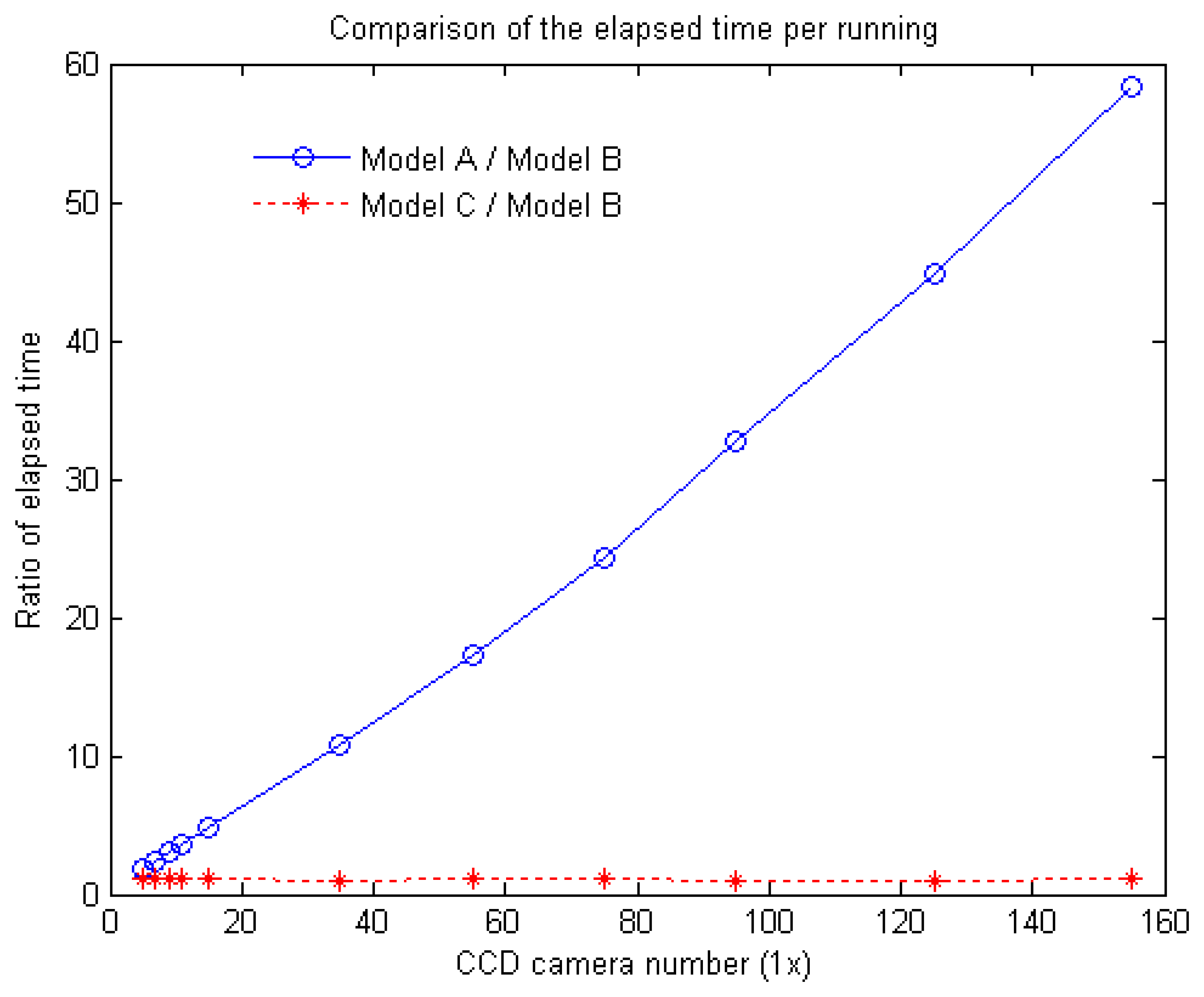
However, if we set a base with Model B, Fig. 6 demonstrates comparison of the ratios of the elapsed time of Models A and C to Model B versus the CCD camera number. The ratios of the elapsed time of Model A to Model B in 1×5, 1×75, and 1×155 are 1.85, 24.35, and 58.25, while the ratios of Model C to Model B are 1.14, 1.19 and 1.05. When the CCD number increases, the ratio of Model C to Model B becomes near constant, which is independent with the CCD amount. But the ratio of Model A to Model B turns to be an oblique curve varying with the CCD amount. In General, the executing time is directly related to the dimensions of image matrix and optical flow vector. Therefore, when the CCD camera number becomes large, in terms of elapsed time it is very obviously that Model B is the best, Model C, close to Model B, is next, and Model A is the worst.
To sum up, from the above comparison on the accuracy and computation efficiency of the single row SPCE with fifty points depicted in Figs. 5 and 6, although Model B has the best computation efficiency, its performance is the worst. While Model A owns best performance only limited in fewer test points, and its computation efficiency is the worst. Therefore, it can be concluded that Model C is the better choice among those three models.
5.2. Variations of Noise Levels
According to previous examination, Model C appears to be the best motion model in noise-resistance capability. Hence Model C is selected for further investigation for motion recovery of the ego-translation movement. Table 2 lists the relative errors for single-row SPCE arrangements under the effect of different noise levels. Promising performance in terms of noise immunity using multiple CCD cameras arranged in single-row SPCE configurations is clearly demonstrated.
For different CCD numbers of the single row SPCE from 1×3 to 1×25, when the variance of noise increases from 1 to 100, the relative error for motion estimation of the ego-translation is enhanced by 10 times in average. This trend is reasonable, because the variance of the noise is proportional to the square of the corresponding component.
Regardless of the magnitude of noise level, the noise interference damages image patterns when the CCD number is small. Besides, the capability of noise-resistance becomes better when the CCD number increases. When the variance reaches 100, the relative error of ego-translation in 1×3 configuration is up to almost 50%. Using the single-row SPCE framework, the relative error can fall down to less than 2% by just modifying the CCD arrangement to 1×25. It can be concluded under the influence of noise interference, when the CCD number increases, the relative error will be greatly reduced. The multiple camera scheme, inspired by the compound eyes of insects, successfully provides outstanding filtering performance on image patterns with noises.
5.3. Irregular Arrangements
The above validations in sections 5.1 and 5.2 are based on regular arrangement of single row SPCE. But what happen if the arrangement of SPCE is irregular? We just made a small deviation for the most left CCD camera in each case of Table 2, and moved its locations to the right hand side 10 mm away from the original position. Table 3 lists the relative errors for the single-row SPCE configuration but with irregular arrangement under the effect of different noise levels. It is very clearly to realize that the irregular arrangement of single row SPCE generated massive relative error comparing to regular arrangement in Table 2.
From Table 3, a number of summaries can be made as follows
- 1)
- When the CCD camera number increases, the relative error becomes larger. Since the deviation is far away from the origin of the coordinate, the relative error will be large. The more of the amount of CCD is, the more of the relative error becomes. For example in 1×25, the relative errors in each case are almost about 120%.
- 2)
- Although under the different level noises, this irregular arrangement of the single row SPCE still dominates the relative error of motion estimation. Thus, the relative errors of the same single row SPCE configuration are close. Exception in 1×3, since the amount of CCD number is too fewer, the relative errors are dominated by the noises of different level variances.
- 3)
- Although the irregular arrangement of the single row SPCE happened with small deviation, the accuracy of estimation for the translation motion is destroyed seriously. Therefore, the regular arrangement is very important in compound eye of an insect for the motion estimation.
5.4. Discussions
From the above experimental results of the single row SPCE, when the CCD's number in the single row SPCE framework increases, the relative error of ego-translation will significantly reduce. If the number of the CCD goes to infinity, the relative error is expected to approach to zero. The SPCE appears to own a powerful capability to overcome noises. In particular, even when the variance of noise is large, the images blurred, the SPCE can still show its effective noise-resistance capability to recover the motion parameters of the translational movement.
The dragonfly has nearly 30000 ommatidia in each eye, which makes sense because they hunt in flight, whereas butterflies and moths, which do not hunt in flight, only own 12000 to 17000 ommatidia [12]. The only difference is the amount of ommatidia. In these situations, due to the increase of the number of ommatidium, the detection accuracy of compound eyes becomes more and more enhanced. It appears that the compound eye is able to provide a more correct detection capability in 3D ego-motion. This phenomenon clearly corresponds to the above experimental results.
Apparently, some of the reasons why the compound eye of the insect is able to help capturing its prey so exactly and quickly are its symmetrical and regular arrangement framework, and its sufficient large number of ommatidia. The multiple camera schemes contribute multiple visual measurements for image patterns that behave like an inherent filter for possible noises. Based on the sufficient multiple image patterns, powerful capability of noise-resistance for motion recovery can be accomplished without using any types of additional signal filters.
6. Conclusions
The compound eyes of the flying insect in the biological world are highly evolved organs. Although the images received from their views are vague and unclear, they are still able to capture prey so exactly and quickly. Inspired by these insects, using pinhole image formation geometry to investigate the visual mechanism of the SPCE to moving objects was conducted.
The principle of the parallel trinocular was first introduced. After extending to the single row SPCE, the experiments for motion recovery of the translational movement under the influence of noises were extensively performed. Especially, a compromised translation motion model is proposed to provide the excellent motion recovery performance with the most accuracy and the faster computation efficiency. Meanwhile, the experimental results also indicate that no matter whether the noise is large or small, the relative error of the ego-translation reduces when the amount of CCD number of the single row SPCE increases. This outcome also lays the basic theoretical foundation to explain why the compound eye of the insect can seize the prey with a tremendous efficiency from the engineering point of view.
Acknowledgments
This work was supported in part by the National Science Council of the Republic of China under Grant NSC 93-2212-E-110-014.
Appendix A
Proof:
For an arbitrary point P in 3D space as shown in Fig. 2, it will project onto the left, middle, and right image planes and the relationships among those three projections can be formulated as
For any two sets for matching image pixels on three different image planes, i.e., (xli, xmi, xri) and (xlj, xmj, xrj),
therefore
It should be noted that the above equation is guaranteed no matter whether h1 is equal to h2 or not.
Appendix B
Proof:
Appendix C
a1b2 − a2b1 ≠ 0
Proof:
Appendix D
a1b3 − a3b1 = 0
Proof:
Appendix E
Proof:
b1c3 − b3c1 = 0, a1c3 − a3c1 = 0 and b1c2 − b2c1 ≠ 0, a1c2 − a2c1 ≠ 0
In addition, a1b2-a2b1 ¹0 is already verified in Appendix C. As a result, the determinant of ATA is proved to be always positive.
Appendix F
Model A:
Model B:
order of A = [(n − 1) + 1] × 3 = n×3, order of d = [(n − 1) + 1] × 1 = n×1
Model C:
order of A = 2(n − 1) × 3, order of d = 2(n − 1) × 1
References and Notes
- Tanida, J.; Kumagai, T.; Yamada, K.; Miyatake, S.; Ishida, K.; Morimoto, T.; Kondou, N.; Miyazaki, D.; Ichioka, Y. Thin observation module by bound optics (TOMBO): Concept and experimental verification. Applied Optics 2001, 40(11), 1806–1813. [Google Scholar]
- Ng, R.; Levoy, M.; Bredif, M.; Duval, G.; Horowitz, M.; Hanrahan, P. Light field photography with a hand-held plenoptic camera. In Computer Science Tech. Rep. CSTR 2005-02; 2005; Stanford University: Stanford, CA. [Google Scholar]
- Adelson, E. H.; Wang, J. Y. A. Single lens stereo with a plenoptic camera. IEEE Trans. Pattern Analysis and Machine Intelligence 1992, 14(2), 99–106. [Google Scholar]
- Netter, T.; Franceschini, N. A robotic aircraft that follows terrain using a neuro-morphic eye. Proc. IEEE /RSJ Int. Conf. Intelligent Robots and Systems 2002, 129–134. [Google Scholar]
- Hoshino, K.; Mura, F.; Morii, H.; Suematsu, K.; Shimoyama, I. A small-sized panoramic scanning visual sensor inspired by the fly's compound eye. Proc. IEEE Int. Conf. Robotics and Automation 1998, 1641–1646. [Google Scholar]
- Volkel, R.; Eisner, M.; Weible, K. J. Miniaturized imaging systems. Microelectronic Engineering 2003. [Google Scholar]
- Hornsey, R.; Thomas, P.; Wong, W.; Pepic, S.; Yip, K.; Krishnasamy, R. Electronic compound eye image sensor: construction and calibration. In Sensors and Camera Systems for Scientific, Industrial, and Digital Photography Applications; 2004; Proc. SPIE 5301; vol. V, pp. 13–24. [Google Scholar]
- Neumann, J.; Fermuller, C.; Aloimonos, Y.; Brajovic, V. Compound eye sensor for 3D ego motion estimation. Proc. IEEE/RSJ Int. Conf. Intelligent Robots and Systems 2004, 4, 3712–3717. [Google Scholar]
- Kim, J.; Jeong, K.H.; Lee, L.P. Artificial ommatidia by self-aligned microlenses and waveguides. Optics Letters 2005, 30(1), 5–7. [Google Scholar]
- Tisse, C.L. Low-cost miniature wide-angle imaging for self-motion estimation. Optics Express 2005, 13(16), 6061–6072. [Google Scholar]
- Kimball, J. W. The Compound Eye, Kimball's Biology Pages. Author website: http://users.rcn.com/jkimball.ma.ultranet/BiologyPages/C/CompoundEye.html.
- Elwell, M.; Wen, L. The power of compound eyes. Optics & Photonics News 1991, 58–59. [Google Scholar]
- Horridge, G.A. A theory of insect vision: velocity parallax. Proc. of the Royal Society of London B 1986, 229(1254), 13–27. [Google Scholar]
- Sobel, E.C. The locust's use of motion parallax to estimate distance. J. Comp. Physiol. A 1990, 167, 579–588. [Google Scholar]
- Srinivasan, M.V.; Zhang, S.W.; Lehrer, M.; Collett, T.S. Honeybee navigation en route to the goal: Visual flight control and odometry. The Journal of Experimental Biology 1996, 199(1), 237–244. [Google Scholar]
- Collett, T. Animal behaviour: Survey flights in honeybees. Nature 2000, 403, 488–489. [Google Scholar]
- Lin, G.L.; Cheng, C.C. Determining 3-D translational motion by the parallel trinocular. Proc. IEEE International Conference on Robotics and Biomimetics 2006, 773–778. [Google Scholar]
- Romoser, W. S. The Science of Entomology; New York; Macmillian Publishing, 1973; pp. 134–138. [Google Scholar]
- Land, M. F.; Nilsson, D.-E. Animal Eyes; New York; Oxford University Press, 2002; pp. 125–131. [Google Scholar]
- Aloimonos, Y. New camera technology: Eyes from eyes. Author website: http://www.cfar.umd.edu/∼yiannis/resaerch.html.
- Simoncelli, E.; Adelson, E.; Heeger, D. Probability distributions of optical flow. Proc. IEEE Int. Conf. Computer Vision and Pattern Recognition 1991, 310–315. [Google Scholar]
- Barron, J.L.; Fleet, D.J.; Beauchemin, S.S. Performance of optical flow techniques. International Journal of Computer Vision 1994, 13(1), 43–77. [Google Scholar]
- Gupta, N.; Kanal, L. 3-D motion estimation from motion field. Artificial Intelligence 1995, 78, 45–86. [Google Scholar]
- Earnshaw, A.M.; Blostein, S.D. The performance of camera translation direction estimators from optical flow: Analysis, comparison, and theoretical limits. IEEE Trans. Pattern Analysis and Machine Intelligence 1996, 18(9), 927–932. [Google Scholar]
- Garcia, C.; Tziritas, G. Optimal projection of 2-D displacements for 3-D translational motion estimation. Image and Vision Computing 2002, 20, 793–804. [Google Scholar]
- Lobo, N.D.V.; Tsotsos, J.K. Computing egomotion and detecting independent motion from image motion using collinear points. Computer Vision and Image Understanding 1996, 64(1), 21–52. [Google Scholar]
- Li, L.; Duncan, J.H. 3-D translational motion and structure from binocular image flows. IEEE Trans. Pattern Analysis and Machine Intelligence 1993, 15(7), 657–667. [Google Scholar]
- Weng, J.; Huang, T.S.; Ahuja, N. Motion and structure from two perspective views: algorithms, error analysis, and error estimation. IEEE Trans. Pattern Analysis and Machine Intelligence 1989, 11, 451–476. [Google Scholar]
Figure 1.
(a) The planar compound-like eye, (b) The single-row planar compound-like eye.

Figure 2.
Schematic for the parallel trinocular.

Figure 3.
A synthesized cloud of fifty 3D points.

Figure 4.
The image points with different noise variances for the 1×25 single-row SPCE before (black) and after (red) a movement.
Figure 4.
The image points with different noise variances for the 1×25 single-row SPCE before (black) and after (red) a movement.
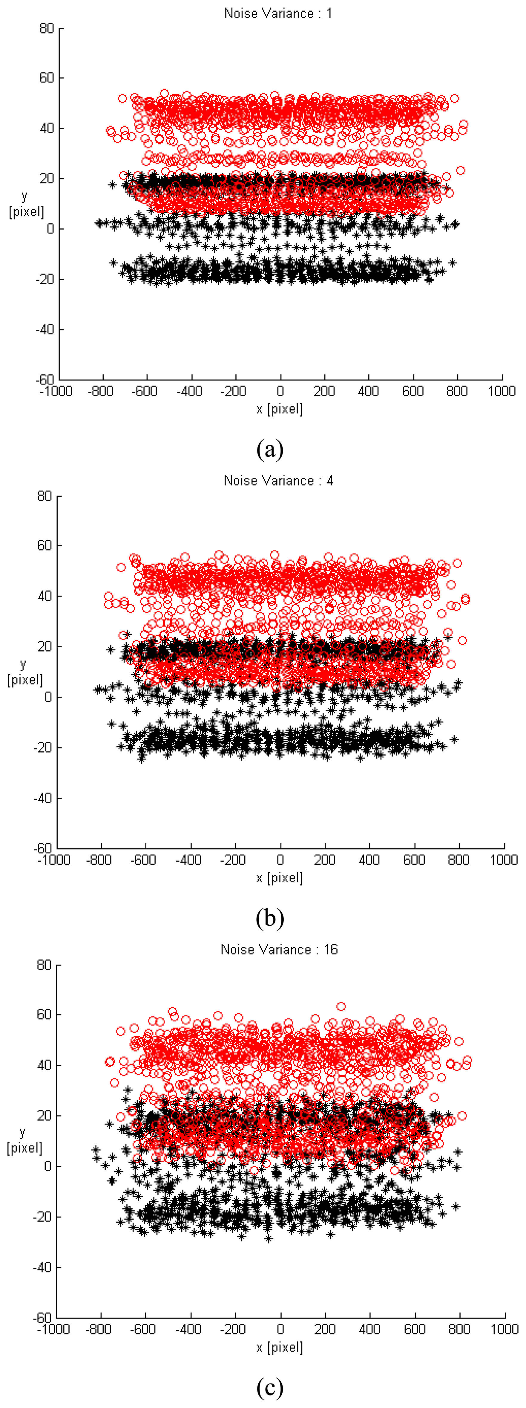
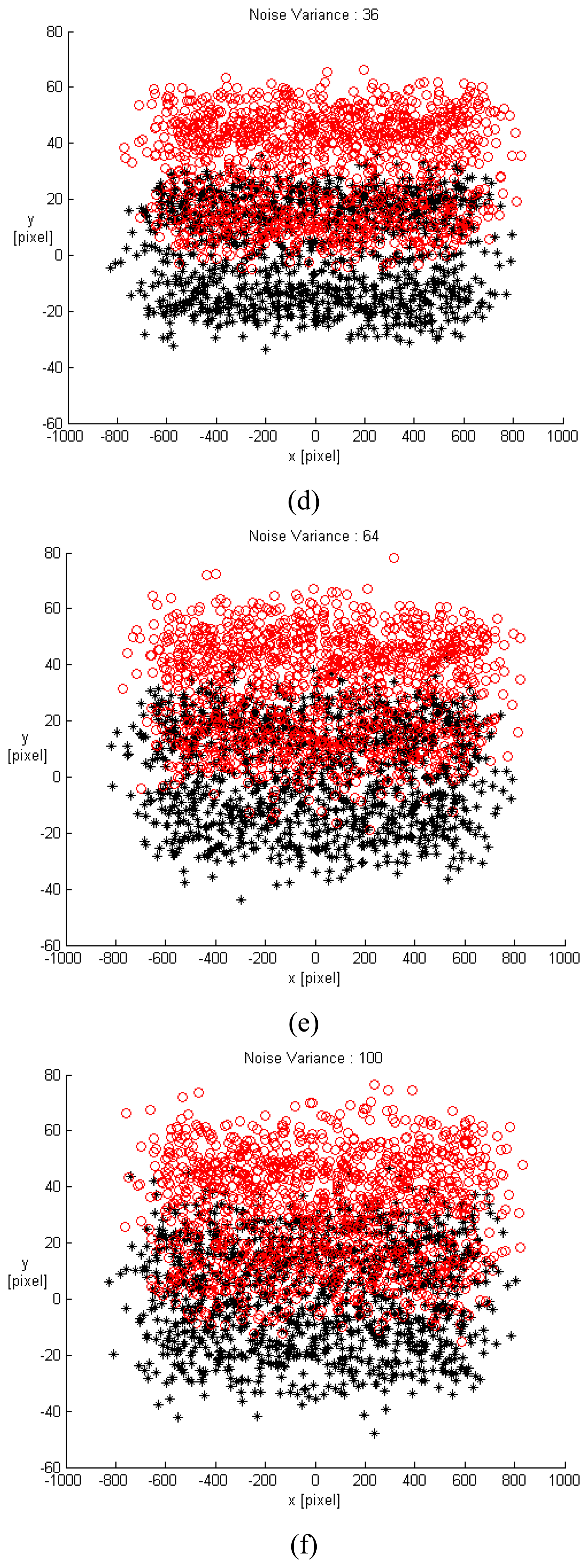
Figure 5.
The relative errors of translation motion in three models with a single, five, and fifty 3D points under a noise level of variance 100.
Figure 5.
The relative errors of translation motion in three models with a single, five, and fifty 3D points under a noise level of variance 100.
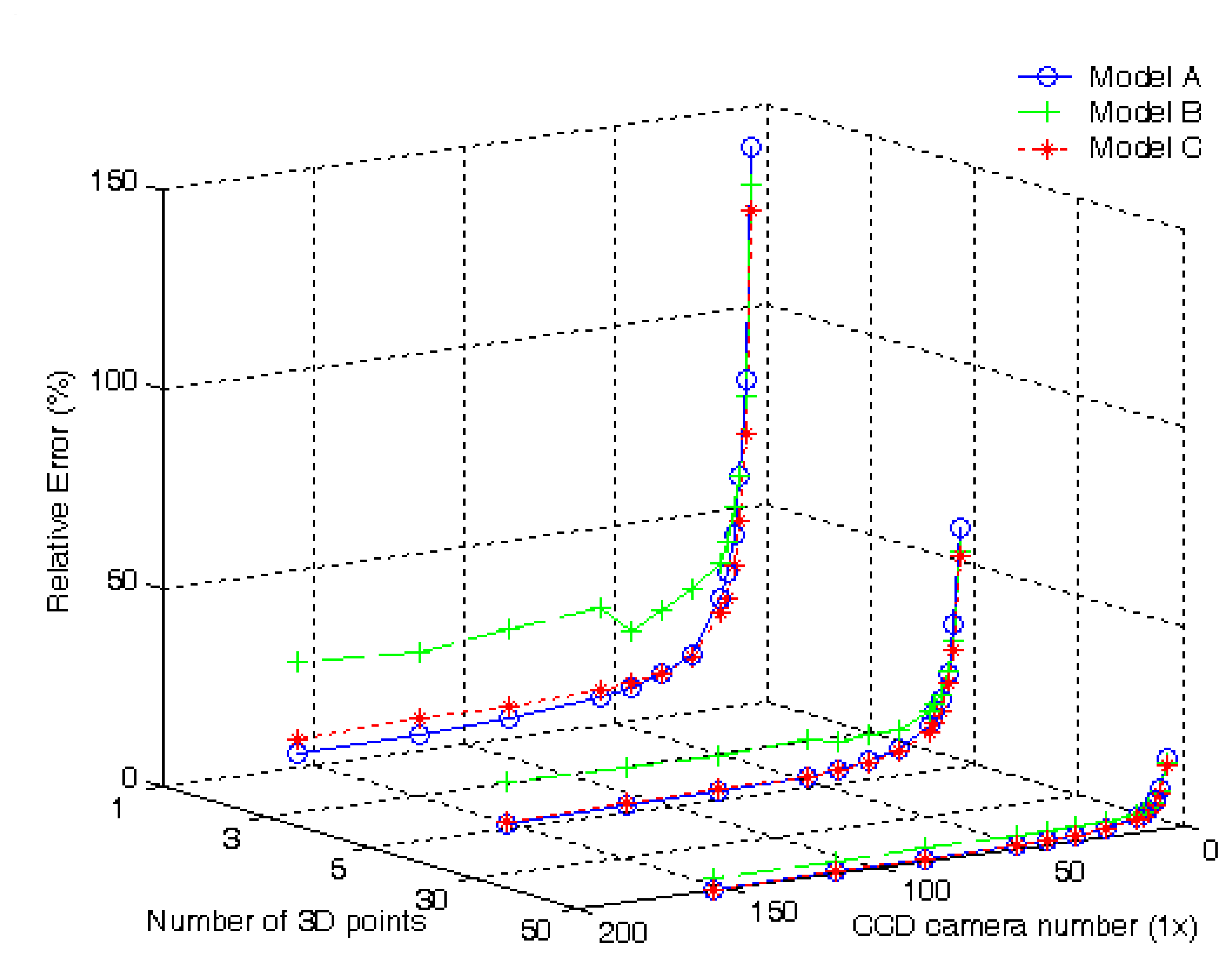
Figure 6.
The elapsed time per running of translation motion in three Models with fifty 3D points under a noise level of variance 100.
Figure 6.
The elapsed time per running of translation motion in three Models with fifty 3D points under a noise level of variance 100.

Table 1.
Elapsed time in sec of the ego-translation for different single-row SPCE configurations with three models under a noise level of variance 100.
| Model | Single-row SPCE configurations | |||||||
|---|---|---|---|---|---|---|---|---|
| 1×5 | 1×15 | 1×35 | 1×55 | 1×75 | 1×95 | 1×125 | 1×155 | |
| A | 0.13 | 1.05 | 5.57 | 14.15 | 27.52 | 46.56 | 83.37 | 153.2 |
| B | 0.07 | 0.22 | 0.52 | 0.82 | 1.13 | 1.42 | 1.86 | 2.63 |
| C | 0.08 | 0.24 | 0.53 | 0.98 | 1.34 | 1.48 | 1.95 | 2.77 |
Table 2.
Relative errors in percent of the ego-translation for different single-row SPCE configurations with various noise variances.
| Noise Variances | Single-row SPCE configurations | |||||||
|---|---|---|---|---|---|---|---|---|
| 1×3 | 1×5 | 1×7 | 1×9 | 1×11 | 1×13 | 1×15 | 1×25 | |
| 1 | 4.69 | 1.50 | 0.90 | 0.60 | 0.42 | 0.36 | 0.30 | 0.16 |
| 4 | 10.01 | 2.82 | 1.62 | 1.19 | 0.80 | 0.68 | 0.62 | 0.33 |
| 16 | 19.51 | 6.43 | 3.74 | 2.25 | 1.72 | 1.35 | 1.14 | 0.68 |
| 36 | 28.18 | 9.59 | 4.91 | 3.68 | 2.60 | 2.00 | 1.74 | 0.95 |
| 64 | 40.13 | 12.43 | 6.15 | 4.59 | 3.74 | 2.81 | 2.26 | 1.34 |
| 100 | 47.85 | 14.03 | 8.79 | 5.81 | 4.18 | 3.60 | 2.89 | 1.58 |
Table 3.
Relative errors in percent of the ego-translation for different single-row SPCE configurations with various noise variances after a small deviation.
| Noise Variances | Single-row SPCE configurations | |||||||
|---|---|---|---|---|---|---|---|---|
| 1×3 | 1×5 | 1×7 | 1×9 | 1×11 | 1×13 | 1×15 | 1×25 | |
| 1 | 3.90 | 54.23 | 67.87 | 75.58 | 81.91 | 87.74 | 93.81 | 120.0 |
| 4 | 8.25 | 54.30 | 67.96 | 75.58 | 81.85 | 87.76 | 93.83 | 120.0 |
| 16 | 16.01 | 54.47 | 67.91 | 75.62 | 81.89 | 87.79 | 93.86 | 120.1 |
| 36 | 23.59 | 54.65 | 67.99 | 75.58 | 81.56 | 87.83 | 93.89 | 120.1 |
| 64 | 32.28 | 54.83 | 67.98 | 75.41 | 82.01 | 87.82 | 93.93 | 120.1 |
| 100 | 40.31 | 54.98 | 68.07 | 75.53 | 82.00 | 87.89 | 93.97 | 120.1 |
© 2007 by MDPI ( http://www.mdpi.org). Reproduction is permitted for noncommercial purposes.
Share and Cite
MDPI and ACS Style
Cheng, C.-C.; Lin, G.-L. Motion Estimation Using the Single-row Superposition-type Planar Compound-like Eye. Sensors 2007, 7, 1047-1068. https://doi.org/10.3390/s7071047
AMA Style
Cheng C-C, Lin G-L. Motion Estimation Using the Single-row Superposition-type Planar Compound-like Eye. Sensors. 2007; 7(7):1047-1068. https://doi.org/10.3390/s7071047
Chicago/Turabian StyleCheng, Chi-Cheng, and Gwo-Long Lin. 2007. "Motion Estimation Using the Single-row Superposition-type Planar Compound-like Eye" Sensors 7, no. 7: 1047-1068. https://doi.org/10.3390/s7071047