Airborne Laser Scanning of Forest Stem Volume in a Mountainous Environment

1
Christian Doppler Laboratory for “Spatial Data from Laser Scanning and Remote Sensing”, at the Institute of Photogrammetry and Remote Sensing, Vienna University of Technology, Gußhausstraße 27-29, 1040 Vienna, Austria
2
Institute of Photogrammetry and Remote Sensing, Vienna University of Technology, Gußhausstraße 27-29, 1040 Vienna, Austria
3
Stand Montafon Forstfonds, Montafonerstraße 21, 6780 Schruns, Austria
4
Department of Forest Inventory at the Federal Research and Training Center for Forests, Natural Hazards and Landscape, Seckendorff-Gudent-Weg, 1130 Vienna, Austria
*
Author to whom correspondence should be addressed.
Sensors 2007, 7(8), 1559-1577; https://doi.org/10.3390/s7081559
Submission received: 20 July 2007
/
Accepted: 14 August 2007
/
Published: 17 August 2007
(This article belongs to the Special Issue Remote Sensing of Land Surface Properties, Patterns and Processes)
Abstract
:Airborne laser scanning (ALS) is an active remote sensing technique that uses the time-of-flight measurement principle to capture the three-dimensional structure of the earth's surface with pulsed lasers that transmit nanosecond-long laser pulses with a high pulse repetition frequency. Over forested areas most of the laser pulses are reflected by the leaves and branches of the trees, but a certain fraction of the laser pulses reaches the forest floor through small gaps in the canopy. Thus it is possible to reconstruct both the three-dimensional structure of the forest canopy and the terrain surface. For the retrieval of quantitative forest parameters such as stem volume or biomass it is necessary to use models that combine ALS with inventory data. One approach is to use multiplicative regression models that are trained with local inventory data. This method has been widely applied over boreal forest regions, but so far little experience exists with applying this method for mapping alpine forest. In this study the transferability of this approach to a 128 km2 large mountainous region in Vorarlberg, Austria, was evaluated. For the calibration of the model, inventory data as operationally collected by Austrian foresters were used. Despite these inventory data are based on variable sample plot sizes, they could be used for mapping stem volume for the entire alpine study area. The coefficient of determination R2 was 0.85 and the root mean square error (RMSE) 90.9 m3ha−1 (relative error of 21.4%) which is comparable to results of ALS studies conducted over topographically less complex environments. Due to the increasing availability, ALS data could become an operational part of Austrian's forest inventories.
1. Introduction
Airborne laser scanning (ALS), also referred to as Light Detection and Ranging (LiDAR), is an active remote sensing technique that has found widespread use in topographic mapping [1-3]. The technical capabilities of ALS sensors have increased rapidly since the mid-1990's when the first commercial systems were introduced into the market [4]. Novel topographic airborne laser scanners typically emit very short (3-10 ns), narrow-beamwidth (0.3-2.0 mrad), infrared (0.80-1.55 μm) laser pulses at near nadir incidence angles (≤ 30°) with a high pulse repetition frequency (50-200 kHz). When operated at altitudes of around 500 to 3,000 m, ALS sensors generate a dense sampling pattern (0.5-20 pulses per m2) of small-footprint (< 1 m) laser pulses on the ground. A small part of the pulse energy is typically scattered backwards towards the sensor where a photodiode registers the time of arrival and, optionally the intensity of the echoes [5]. Thus the ranges (distances) between the sensor and the objects, which generated the backscattered echoes, can be determined. The result of this measurement process is a 3D point cloud which needs to be further interpreted before becoming useful in applications [6].
Over vegetated terrain most of the laser pulses are reflected by the leaves and branches of the vegetation canopy [7, 8]. However, a certain fraction of the pulses reaches the ground surface through small openings in the vegetation canopy. By using filtering techniques to separate terrain echoes from vegetation echoes it becomes possible to reconstruct the terrain surface [9]. This unique capability of ALS to directly measure the terrain height also in forested areas [10] has been an important reason for the quick adoption of ALS for collecting high precision digital terrain models (DTMs).
By subtracting the terrain height from the vertical coordinate of the 3D point cloud, a virtual representation of the vegetation canopy is obtained. The significant potential of this 3D canopy representation for forestry applications, including estimation of canopy heights, stand volume, basal area or above-ground biomass has been pointed out repeatedly [11-14]. But still, ALS is not yet widely used in an operational context [15]. Besides economic and organizational aspects, there are methodological reasons that may explain the comparably slow adoption of ALS in operational forestry applications. One problem is that models are required to transform the point cloud into geophysical forest parameters. Even though research must strive to develop generic models, one has to expect that these models have to be adapted to different tree species and environmental conditions [16].
Much research on the use of ALS for forestry applications has so far focused on boreal forests. In Scandinavia the operational use of ALS data within forest inventories has become a reality [13, 17]. Probably the most widely used method for deriving various forest parameter is a statistically-based multiplicative regression model, as published by Næsset [18-20]. This multiplicative regression model must be trained with local inventory data and uses various statistical quantities derived from the ALS point cloud, including mean values, coefficients of variation, percentiles of heights, and canopy densities.
The aim of this study has been to investigate the transferability of this multiplicative regression model for mapping of alpine forests. A 128 km2 mountainous area in the western part of Austria was selected as study area. In Austria, ALS data covering large alpine areas have only become available recently. Despite the complex mountainous topography, the ALS derived terrain and canopy height models are of good quality as the investigation by Hollaus et al. [21] has shown. However, the transfer of the multiplicative regression model may still be hampered or even be impeded by the fact that the structure and properties of alpine forests is quite different from boreal ones. Also, the transfer may be made difficult in practice because Austrian foresters routinely use an inventory method that is not well adapted for matching the ground measurements with remote sensing data. This inventory method is based on so-called Bitterlich plots which are characterized by variable sample plot sizes. For each sample plot the selection of trees, which are used for the measurements, depends on the diameter at breast height in dependence of the distance between the sample plot center and the tree [22]. The Austrian inventory method is discussed in more detail in Section 2, after the description of the study area and ALS datasets. The pre-processing of the ALS data and the multiplicative regression model are described in Section 3 and 4 respectively, followed by the presentation of the results in Sections 5. The impacts of different ALS flight specifications and the perspectives of using ALS intensity and full-waveform data are discussed in Section 6 and 7.
2. Study area and data
2.1 Study area
The study area is situated in the southern part of the federal state of Vorarlberg, Austria (Figure 1) and covers 128 km2 of the Montafon region. The complex alpine landscape of the study area has high relief energy, whereas the elevations range between 800 and 2,900 m. The land cover is characterized by coniferous and mixed forests, shrubs, meadows, and sparsely settled areas in the valley floors. According to the Stand Montafon Forstfonds1 the main tree species in the area are spruce (Picea abies) with 96% and fir (Abies alba) with 3%. Especially in valleys and sunny slopes, mixed forests with the species red beech (Fagus sylvatica) can be found. The mean stem volume of the Montafon region is 465 m3ha−1, which is high compared to 325 m3ha−1 2 representing the average Austrian stem volume. Two thirds of the forests are located above 1,000 m sea level, whereas the timberline is at about 1,950 m. As a result of the mountainous terrain 6% of the forests grow on a slope inclination of more than 45°, and 61% between 30° and 45°. Furthermore, 28% of the forests grow on slopes between 15° and 30°, and only 5% on slopes less than 15°. Approximately 80% of the forested area is managed forest with a protection function (protection forest with yield), 10% is managed forest (commercial forest), and the rest is unmanaged protection forest (protection forest without yield) on extreme sites or at the timberline. In alpine regions protection forests are of great importance to protect inhabited areas, roads and railway lines from natural hazards such as rockfalls and snow avalanches. About half of the forests in the study area are managed by the forest administration Stand Montafon Forstfonds, which is the largest forest owner in Vorarlberg. They operate a precise forest inventory, which provides the field data used in this study. The forested areas managed by the Stand Montafon Forstfonds are regularly distributed over the entire test site and therefore, this forest inventory data are representative for the entire study area. Within the study area the average forest stand size is approximately 3.5 ha and is equal to the average area of private owned forests in Austria.
2.2 Airborne laser scanner data
The ALS data were acquired in the framework of a commercial terrain mapping project during two flight-campaigns. The first flight took place on December 10, 2002 (snow-free, leaf-off) and covers the lower altitudes, the second on July 19, 2003 and covers the higher altitudes (snow-free, leaf-on) as shown in Figure 1. The data cover the whole study area and are characterized by an average density of laser hits of 0.9 points per m2 and 2.7 points per m2, respectively. For both flights the flying heights above ground range between ∽650 m and ∽2,000 m, whereas the average flying height was 1,000 m. For the winter flight an Airborne Laser Terrain Mapper (ALTM i1225) and for the summer flight an ALTM 2050 was used. The beam divergence for both systems is 0.3 mrad, which results in a mean footprint size of 0.3 m for the average flying height. The maximum scan angle was ±20 deg. During both flight-campaigns 650 millions laser scanner points were acquired, including first- and last-echoes. Further information about the used data sets can be found in Wagner et al. [23].
2.3. Forest inventory data
The forest inventory data are provided by the forest administration Stand Montafon Forstfonds, which operates a precise inventory since 1988 for approx. 65 km2 forests in the southern part of Vorarlberg, in the so-called Montafon region. The design of this inventory is based on permanent sample plots distributed in a regularly 350 m grid (Figure 1). The inventory data used in this investigation were collected at 143 inventory sample plot in the year 2002. For each plot trees were selected according to the Bitterlich method, which is a so-called probability-proportional-to-size sampling method, meaning that the probability of selection is proportional to tree basal area [22]. It is a point sampling method and, therefore, it does not refer to a certain sample plot area. A relascope with a relascopic factor of four (angle gauge) was used for the selection of the sample trees.
For all selected trees, the tree species was determined and the diameter at breast height (dbh) was measured with a tree caliper at the breast height of 1.3 m. For trees with a dbh greater than 1.0 m the dbh were measured with a diameter tape. Trees with a dbh less than 0.1 m were excluded from this forest inventory, which is a common practice in Austria.
For each sample plot one tree height (h) for each tree species was measured with a Vertex III hypsometer3. For the selection of the tree, whose height is measured, the 50% mark in the stand basal area distribution is used. If there were more than 10 trees with the same tree species, the heights of two trees were measured. If the selected trees within a sample plot were grouped to two clearly differentiable tree height clusters, for each height cluster one tree height was measured. The heights of the remaining sample trees are calculated by means of height curves, which describe the relationship between h and dbh. For the available forest inventory data the height curve according to Keylwerth [24] is used, which is defined by the following mathematical function:
where h is the tree height in meters, a0 is a variable coefficient, a1 is a constant coefficient, and dbh is the tree diameter at breast height (1.3 m) in centimeters. The coefficient a0 depends on the site quality and is calculated by means of the measured h-dbh pair for each sample plot and each tree species separately. Knowing a0 for each sample plot all the missing tree heights within the plot are calculated. The expected standard deviation of the estimated heights ranges between 1.3 and 1.9 m [25].
For the calibration of the ALS data the stem volumes per unit area are used as ground reference quantities. The estimation of stem volume is based on regional volume equations of the Bavarian forest inventory, as these reflect the growth pattern of spruce in the province of Vorarlberg best. These volume equations are based on a so-called form height concept, which means that the conical shape of the stems is transformed to a cylinder. The diameter of the cylinder corresponds to the dbh and the height (form height (FH)) is calculated by means of the following formula [26]:
where FH is the form height in meters, cij are the constants for the different tree species taken from the inventory-evaluation software of Süß [27]. According to Sterba [28] the stem volume (vstem,fi) per ha can be calculated with the following formula:
where vstem,fi is the stem volume in m3ha−1, k is the relascopic factor (set to 4), and n is the number of measured trees per sample plot unit. The calculated vstem,fi corresponds to the commercial useable timber volume and is therefore not equal to the real biological available stem volume within the forest. In contrast to the commercial useable timber volume, the biological one includes additional small trees (dbh < 10 cm) and old trees in bad condition.
3. Data pre-processing
3.1. ALS data pre-processing
The pre-processing of the ALS data includes the georeferencing, the generation of topographic models (e.g. digital terrain and surface model), and the derivation of canopy heights. The georeferencing of the ALS data is based on the method developed by Kager [29]. This method uses an adjustment strategy for correcting the exterior orientation elements as recorded by differential-GPS (dGPS) and an Inertial Measurement Unit (IMU), as well as interior orientation elements concerning the Scanner-dGPS-IMU system. Correction polynomials in the time domain to all degrees of freedom as determined by the dGPS-IMU components and to the relative orientation parameters between those and the laser scanner-device itself are applied. All these parameters are determined simultaneously with hybrid block adjustment by least squares. The derived horizontal errors are below 0.5 m and the vertical DTM errors increase from 0.10 m for relatively flat terrain (local slope <10°) to over 0.50 m for local slopes greater than about 60° [21]. These reported accuracies were derived from non-forested areas within the study area.
The georeferenced 3D point clouds are used to calculate the digital terrain model (DTM), digital surface model (DSM), and the canopy heights. The last-echo points were used for generating the DTM using a hierarchic robust filtering technique described in Briese et al. [30], Kraus and Pfeifer [10], and Pfeifer et al. [31]. The generation of the digital surface model (DSM) is based on the first-echoes. A moving planes interpolation of the highest first-echo points within a pre-defined grid of one meter was applied. This interpolation fits tilted planes into the eight nearest points by using a least square approach. The heights are weighted inversely proportional to the distance from the grid point. The used algorithms are implemented in the software-package Scop++ [31]. The spatial resolution of both topographic models is one meter. The canopy heights were calculated by subtracting the terrain heights from the absolute heights of the first- and the last-echo points respectively. Detailed information regarding the accuracy of the derived terrain and canopy heights can be found in Hollaus et al. [21].
3.2. Co-registration of the forest inventory data to the ALS data
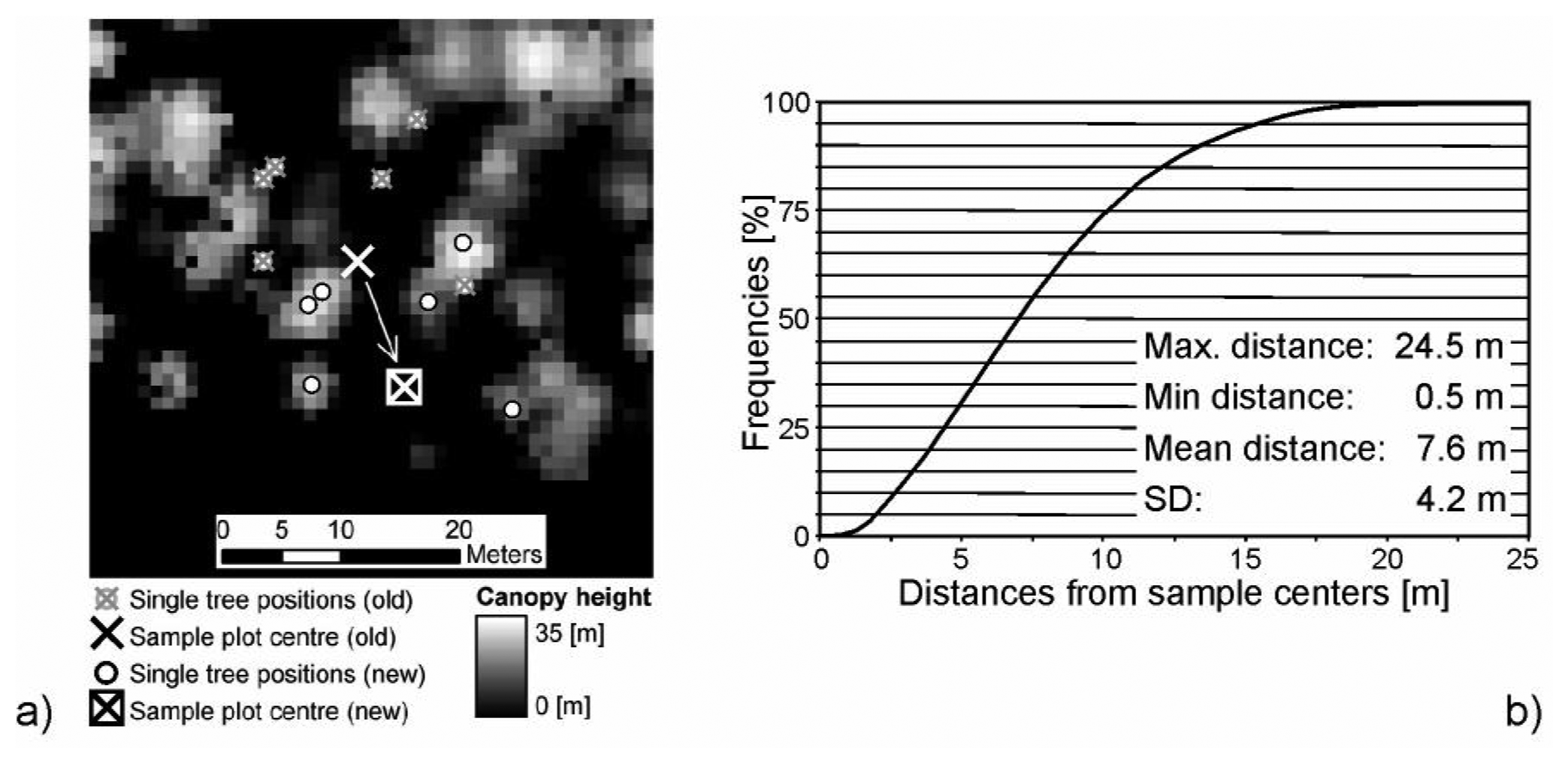
Although the forest inventory is based on permanent sample plots the accuracies of the available coordinates of the sample plot centers vary in the range of several meters. The inaccuracies can be explained by the used surveying instruments (i.e. compass in combination with an ultrasonic range instrument), which were applied for the positioning. About two tens of reference measurements with differential GPS have shown that the average position error is approximately 10 m, which is quite large compared to a 20 m diameter of the sample plots used for the ALS data analyses. To overcome this problem manual co-registration of the forest inventory data to the ALS data has been carried out. For this purpose positions of single trees are needed, which were measured during the forest inventory field campaign. For all sampled trees the polar coordinates relative to the sample plot center were measured with a compass in combination with an ultrasonic range instrument. The expected accuracies of the measured polar coordinates are in the range of 0.3 to 0.5 m. As shown in Figure 2a the position of each sample plot center is adjusted so that the measured single-tree positions best fit to the visual detectable tree positions in the ALS canopy height model (CHM) and that the measured tree heights best fit to the CHM heights. The relative positions of the single-trees within one sample plot are not changed during this co-registration. The CHM is calculated by subtracting the terrain model from the surface model [21]. For the co-registration a maximum possible displacement of 15 m is assumed.
In this way the positions of 103 of the 143 available sample plots could be clearly co-registered to the ALS data. For the further analyses the calculated vstem,fi of these clearly co-registered sample plots are used as reference data. Within the 103 sample plots 925 trees were measured, whereas the dbhs vary between 10 and 127 cm and the tree heights between 5.4 and 42.2 m. The distances of the trees from the sample plot centers vary between 0.5 and 24.5 m as shown in Figure 2b. The average distance is 7.6 m and the standard deviation is 4.2 m. A summary of the available forest inventory data is shown in Table 1.
4. Stem volume estimation
4.1. Multiplicative stem volume model
The multiplicative regression model used for estimating stem volume [20] requires as input the forest inventory data and different statistical quantities derived from first- and last-echo ALS data including mean values, coefficients of variation, percentiles of heights, and canopy densities for several height intervals. The calculations are based on circular sample plot areas, whereas different diameters are evaluated. The model is formulated as:
where Y is the vstem,fi in m3ha-1; h0,f, h10,f, …, h90,f are percentiles of the first-echo laser canopy heights for 0%, 10%, …, 90% in m; h0,1, h10,1, …, h90,1 are percentiles of the last-echo laser canopy heights for 0%, 10%, …, 90% in m; hmean,f, hmean,1 are mean values of the first- and last-echo canopy heights in m; hcv,f, hcv,1 are coefficients of variation of the first- and last-echo canopy heights in percent. As suggested by Næsset [20] and Nilson [32] first- and last-echo returns with heights less than 2 m are classified as ground hits, stones, shrubs, etc., and therefore, the heights are set to zero; d0,f, d1,f, …, d9,f are cumulative canopy densities of first-echo laser points for the fraction no. 0, 1, …, 9; d0,1, d1,l, …, d9,1 are cumulative canopy densities of last-echo laser points for the fraction no. 0, 1, …, 9. The 10 fractions are of equal height and are calculated by dividing the difference between the highest and the lowest (2 m) canopy height by 10. For each fraction no. 0, 1, …, 9 (> 2 m) the proportion of laser hits above the fraction limits to the total number of laser hits were calculated for both, first- and last-echo points. The model parameter of Eq. (7) can be estimated with the linear form of the equation using logarithmic variables as shown in Eq. (8).
4.2. Regression analyses
For the development of the final model stepwise multiple regression analyses is used. Starting with the regression equation, Eq. (8), including all independent variables, a backwards working approach is applied. In this approach variables are dropped out from the equation one at a time if the significance level of the partial F statistic is greater than 0.05. Finally, a co-linearity measure is used for selecting the final variable set, whereas only models whose condition number κ < 30 are accepted. For the stepwise multiple regression analyses the open source software R4 is used.
4.3. Correction of the logarithmic transformation bias
For the multiple regression analysis the multiplicative model (Eq. (7)) is transformed into a logarithmic scale (Eq. (8)). This common procedure has the advantage that the complex multiplicative model can be expressed by a linear one. Thus, a simple least square method can be applied for estimating the model parameters. For the final prediction of the stem volume a conversion of the log-linear model parameters to the original untransformed scale is necessary. This procedure introduces a bias because large values are compressed on the logarithmic scale and thus tend to have less leverage than small ones [33]. Thus, the bias is not an arithmetic constant but a constant fraction of the estimated value. In the current study the empirical ratio estimator (RE) approach developed by Snowdon [34] is used for correcting the bias. As demonstrated by Snowdon [34] this method is more reliable than corrections estimated from variance as for example described by Baskerville [35] or Sprugel [36]. The correction factor for the empirical ratio estimator is calculated as shown in Eq. (9).
4.4. Validation of the stem volume model
Due to the variable sizes of the forest inventory sample plots the appropriate sample plot size to extract the ALS data is not known in advance. Therefore, several diameters are used and evaluated. The sample plot size, which leads to the highest accuracy, is used to analyze the effects of varying ALS properties.
As mentioned in section 2.2, the study area is covered by two ALS data sets with different point densities and acquisition times. The winter ALS data cover 92 and the summer ALS data cover 64 from the 103 forest inventory sample plots, which could clearly be co-registered. Within the overlapping area of the two data sets 52 forest inventory sample plots are available, which are used to analyses the effects of varying acquisition times. As the summer ALS data have a point density of 2.7 p/m2 a thinning of 66% is applied to reduce the density to those of the winter data (0.9 p/m2). Based on the sorted acquisition time the thinning is done by a systematic removal of points.
To understand the impact of different ALS point densities the original and the thinned data are analyzed for each acquisition time separately. Thus, the results can easily compared within each flight campaign as the flying height, the local incidence angles, the acquisition times, the sensor characteristics, and the used sample plots are similar for the original and the thinned data set.
For the validation of the calibrated models a cross-validation procedure is used, where for each step one observation is excluded for the calibration of the model. Since the model is fitted n times, where n is the number of observations, the prediction error for each excluded observation can be calculated. Finally, statistical parameters of the prediction errors can be calculated including the range, the mean, and the standard deviation of the errors.
5. Results
5.1. Sample plot size
For the determination of the appropriate sample plot size five different diameters (18 m, 20 m, 22 m, 24 m, and 26 m) were used. All co-registered sample plots (103) were used for the multiple regression analysis. The final models and statistical parameters of the derived results are shown in Table 2.
A sample plot size with a diameter of 24 m leads to the highest coefficient of determination (R2 = 0.84) and to the lowest root mean square error (RMSE = 96.8 m3ha−1 corresponding to a relative error of 22.9%). The final model consists of three independent variables including h0,f, h30,l and d6,f. The residuals derived from the cross-validation vary between -254.7 and 204.1 m3ha-1 and have a standard deviation of 100.0 m3ha−1.
5.2. Effects of different ALS point densities and acquisition times
The analysis of the effects of different point densities was done for all (103), the winter (92), the summer (64), and the 52 forest inventory sample plots located within the overlapping area of the two data sets separately. Based on the original and on the thinned ALS data sets a circular sample plot with a diameter of 24 m was used. The thinning of the ALS data sets leads to a minor decrease of R2 from 0.84 to 0.82 using all 103 FI sample plots and from 0.81 to 0.77 using only the 92 plots covered by the winter ALS data. For the 64 sample plots covered by the summer data no change of the R2 (R2=0.82) could be observed by thinning the point density of 66%. As it is summarized in Table 3 the RMSEs show inversely proportional tendencies and increase slightly for the thinned data from 96.8 to 104.4 m3ha—1 for all plots, from 110.4 to 117.5 m3ha−1 for the winter plots, and from 97.9 to 99.9 m3ha−1 for the summer plots. Also the standard deviations of the residuals increase from 100.0 to 106.7 m3ha−1 for all plots, from 114.8 to 122.7 m3ha−1 for the winter plots, and from 110.7 to 111.3 m3ha−1 for the summer plots.
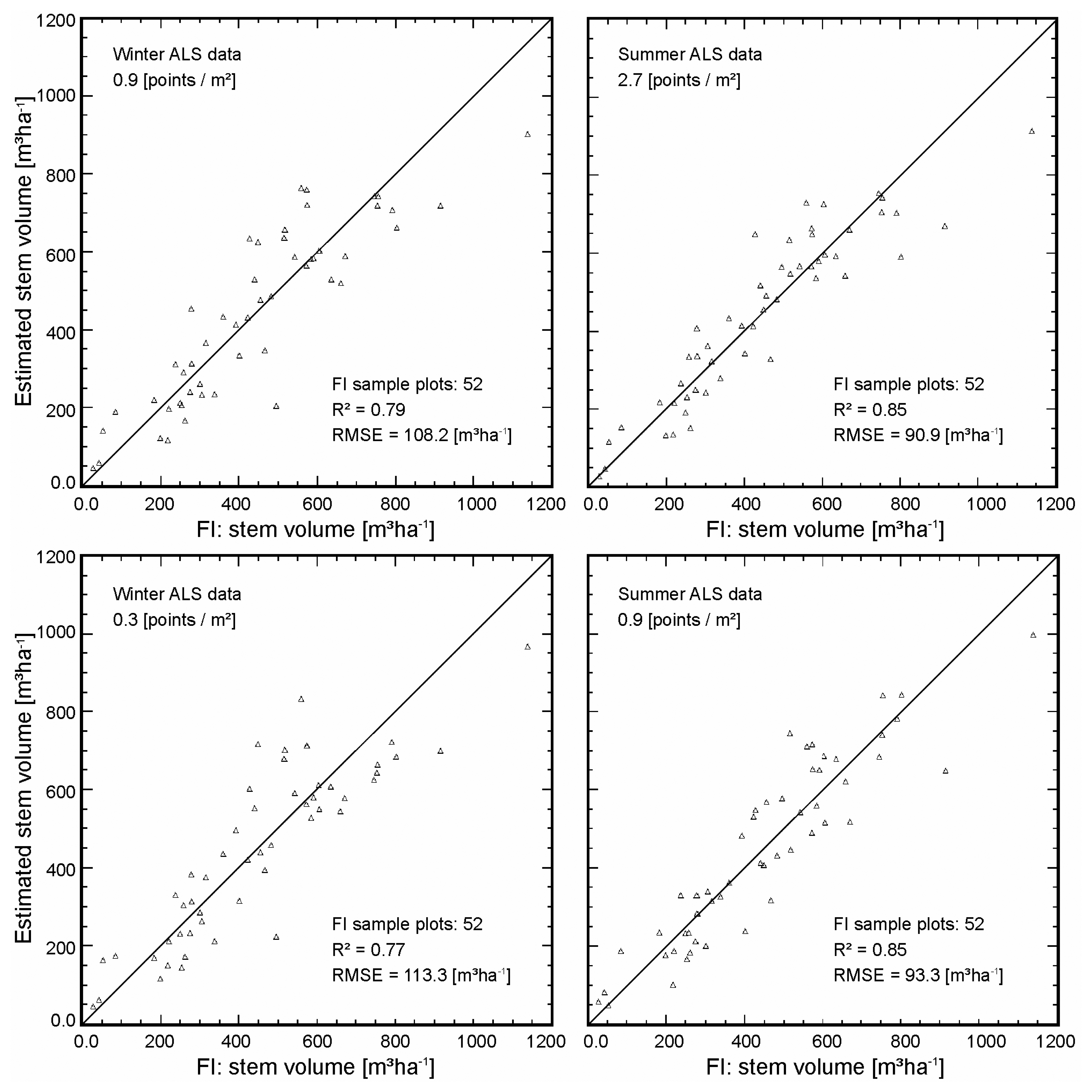
To study the effects of different acquisition times the accuracies of the winter and the thinned summer data are compared. Only those 52 sample plots are used which are covered by the winter and the summer data simultaneously. The achieved R2 is higher for the thinned summer data than for the winter data and are 0.85 and 0.79 respectively. For the RMSE and the standard deviation of the residuals a decrease from the winter to the thinned summer data can be observed. The RMSE decreases from 108.2 to 93.3 m3ha−1 (Figure 3) and the standard deviation from 120.0 to 104.0 m3ha−1 as shown in Table 3.
6. Discussion
6.1. Stem volume model
The results of this study indicate that the multiplicative stem volume model can successfully be applied for a mountainous forest in Austria. The derived coefficient of determination (R2 = 0.84) is comparable with those derived from boreal forests (R2 = 0.83 – 0.97) reported in Næsset [20]. Furthermore, Næsset [20] summarizes that the RMSE of the differences between estimated and ground reference values range from 32.9 to 67.8 m 3ha-1 (17.5 to 22.5%) which is comparable to 96.8 m3ha−1 (22.9%) derived in the current study. As shown in Figure 3 the model fits best for sample plots with lower stem volumes. For higher volumes the model shows some underestimations and therefore, additional improvements would be advisable. A possible way to minimize this shortcoming is to stratify the reference FI plots into several predefined forest classes according to the tree age and site quality, as for example describe in Næsset [20]. This approach requires a higher number of reference data, which consequently enhance the costs for field work. Furthermore, a stratification of the forest is required before the model can be applied. In several studies [37-39] it is demonstrated that the fusion of LiDAR data and optical remotely sensed data provides improved opportunities for such a forest stratification. Also full-waveform ALS data provide in addition to the geometric information physical quantities (e.g. amplitude, echo width, backscatter cross-section), which can be used for tree species classifications [40].
For the operational application of this model it has to be considered that the variables derived from first- and last-echoes are known to change depending on different ALS system parameters. For example, Næsset [41, 42] found that the effects of different flying altitudes on estimated canopy heights and densities are more pronounced for last-echoes than for first-echoes. Similar to the final regression models published in Næsset [20] the final models derived in this study also include variables calculated from both echo types. As already described in section 2.2 the difference between the minimum and the maximum flying heights above ground is about 1,350 m, which is quite large compared to 272 to 535 m used for the studies described in Næsset [20]. These high variations in the flying heights could also explain the slightly lower accuracies derived over this mountainous region.
Concerning the effects of varying ALS point densities this study shows that for each ALS data set an individual model can successfully be fitted as summarized in Table 3. This is confirmed by the small differences of the derived root mean square errors for the original and the thinned winter and summer data. To guarantee that only the point density influences the results, only those sample plots were used, which are located in the overlapping area between winter and summer ALS data. Even tough the differences of the derived root mean square errors between the original and the thinned winter and summer data are small, it was observed that the increase of the RMSE (ΔRMSE = 5.1 m3ha−1) with decreasing point densities from 0.9 to 0.3 p/m2 is slightly higher than those (ΔRMSE = 2.4 m3ha−1) from 2.7 to 0.9 p/m2 (Table 3).
Concerning the different acquisition times the results derived from the winter and the thinned summer data were compared. While similar R2s were derived, the differences of the RMSEs, and the standard deviation of the residuals derived from the cross-validation are relatively large and are 14.9 m3ha−1 and 16.0 m3ha-1 respectively as can be seen in Table 3. For example Gaveau and Hill [43] and Hollaus et al. [21] found that even for coniferous forest the penetration rate of laser pulses to the terrain surface is slightly higher for winter than for summer conditions. Therefore, the summer ALS data provide a higher percentage of canopy points than winter data, which can explain the observed differences for the investigated coniferous forest. A further reason for the varying results could be related to the different sets of the final independent variables derived from the regression analyses (Table 3). Finally, differences in the derived ALS parameters can occur due to the seasonal variation of the undergrowth, which influences the DTM accuracy and therefore the accuracy of the canopy heights [44].
6.2. Forest inventory data
Due to geometric discrepancies between the forest inventory plots and the ALS data a manual co-registration was applied. About two-thirds of the available sample plots could clearly be co-registered to the ALS data. The relative high number of remaining sample plots (n = 40) can be explained by the defined maximal displacements of 15 m. If one would extend the possible displacements ambiguous results can occur. For future applications an improved determination of the sample plot center coordinates (e.g. using dGPS, etc.) is recommended.
Even though the sample plot areas of the forest inventory data were variable, the statistically calculated stem volumes in m3ha−1 could be used for the calibration of the stem volume models. As summarized in Table 2 the influence of the used sample plot size to the achievable accuracies is small.
A critical point of the used forest inventory data is the use of tree height (h) / diameter at breast height (dbh) curves to compute the heights of those trees whose heights were not measured in the field. As describe in section 2.4 for each sample plot a h/dbh curve is calibrated based on the measured h and dbh of the tree with the median dbh and the remaining tree heights were computed based on the calibrated model. A detailed accuracy analysis could not be done due to the missing reference data. Therefore, it is assumed that the calculated stem volumes compensate the uncertainties of the individual tree height calculations by averaging the under- and overestimations. This assumption could be confirmed by the high accuracies that were achieved.
The used forest inventory data do not include trees with a dbh less than 10 cm, corresponding to tree heights less than approximately 5.6 m. Due to the high average stem volume quantities of the current test site (∽473 m3ha−1) the lack of these trees has a minor influence on the calculated stem volumes. Apart from the estimation of the commercial useable timber volume, which is represented by the forest inventory data, the estimation of the real biological available stem volume should consider also trees with a dbh less than 10 cm.
7. Conclusions
The technique of airborne laser scanning has reached the maturity to be of use for large-scale mapping of structural forest parameters in alpine environments. By combing the ALS derived 3D point cloud with forest inventory data in the multiplicative regression model approach used by Næsset [20] it has been possible to map forest stem volume in a 128 km2 large area. The validation showed that R2 is 0.84 and RMSE 96.8 m3ha−1 (22.9%), which is comparable to results derived for boreal forests. The good results obtained in this study offer an operational perspective for the use of ALS data in the Austrian forest inventory, considering that both the ALS and inventory data were collected as part of routine data collection activities. In that respect it is also important that the accuracy of the method decreased only slightly when the laser point density on the ground was decreased from 2.7 to 0.3 points per m2.
Future research will address the question if and how this method can be transferred to other forest ecosystems in Austria using data from the national forest inventory. The Austrian national forest inventory is carried out regularly with a time interval of six to eight years. Today, more than 170 attributes are assessed, which provide information on quantity, quality and trends of the Austrian forests [45]. The challenge will be to match ALS data acquired with different sensors and flight parameters with forest inventory data collected at permanent sample plots, which are systematically distributed in a 3.89 km grid over the entire country.
Also, we plan to investigate the benefits of ALS systems that record the echo intensity or the complete echo waveform [46] for forestry applications. Initial research results indicate that the intensity and waveform data may be useful for classifying coniferous and deciduous tress [40, 47] and for improving the separation of vegetation and terrain echoes [7]. However, much research, e.g. on the calibration of the intensity data [48, 49], still remains to be done before these data can be considered for operational forest applications.
Acknowledgments
We would like to thank the Landesvermessungsamt Feldkirch for granting the use of the ALS data and the forest administration “Stand Montafon Forstfonds” for providing the forest inventory data. Furthermore, we are grateful to our colleagues C. Eberhöfer and H. Kager for the pre-processing of the ALS data. Parts of this study were funded by the Austrian Federal Ministry of Agriculture, Forestry, Environment and Water Management (BMLFUW) in the framework of the project ÖWI-Regio.
References
- Kraus, K.; Karel, W.; Briese, C.; Mandlburger, G. Local Accuracy Measures for Digital Terrain Models. The Photogrammetric Record 2006, 21(116), 342–354. [Google Scholar]
- Chen, Q.; Gong, P.; Baldocchi, D.; Xie, G. Filtering airborne laser scanning data with morphological methods. Photogrammetric Engineering and Remote Sensing 2007, 73(2), 175–185. [Google Scholar]
- Kobler, A.; Pfeifer, N.; Ogrinc, P.; Todorovski, L.; Oštir, K.; Džeroski, S. Repetitive interpolation: A robust algorithm for DTM generation from Aerial Laser Scanner Data in forested terrain. Remote Sensing of Environment 2007, 108(1), 9–23. [Google Scholar]
- Flood, M. Laser Altimetry: From Science to Commercial Lidar Mapping. Photogrammetric Engineering & Remote Sensing 2001, 11, 1209–1217. [Google Scholar]
- Wehr, A.; Lohr, U. Airborne laser scanning - an introduction and overview. ISPRS Journal of Photogrammetry & Remote Sensing 1999, 54, 68–82. [Google Scholar]
- Axelsson, P. Processing of laser scanner data - algorithms and applications. Photogrammetry & Remote Sensing 1999, 54, 138–147. [Google Scholar]
- Wagner, W.; Hollaus, M.; Briese, C.; Ducic, V. 3D vegetation mapping using small-footprint full-waveform airborne laser scanners. International Journal of Remote Sensing 2007, in press. [Google Scholar]
- Goodwin, N. R.; Coops, N. C.; Culvenor, D. S. Development of a simulation model to predict LiDAR interception in forested environments. Remote Sensing of Environment 2007. [Google Scholar] [CrossRef]
- Sithole, G.; Vosselman, G. Experimental comparison of filter algorithms for bare-Earth extraction from airborne laser scanning point clouds. ISPRS Journal of Photogrammetry & Remote Sensing 2004, 59(1-2), 85–101. [Google Scholar]
- Kraus, K.; Pfeifer, N. Determination of terrain models in wooded areas with airborne laser scanner data. ISPRS Journal of Photogrammetry & Remote Sensing 1998, 53(4), 193–203. [Google Scholar]
- Dubayah, R.; Drake, J. Lidar Remote Sensing for Forestry. Journal of Forestry 2000, 98, 44–46. [Google Scholar]
- Lim, K.; Treitz, P.; Wulder, M.; St-Onge, B.; Flood, M. LIDAR remote sensing of forest structure. Progress in Physical Geography 2003, 27(1), 88–106. [Google Scholar]
- Næsset, E.; Gobakken, T.; Holmgren, J.; Hyyppä, H.; Hyyppä, J.; Maltamo, M.; Nilsson, M.; Olsson, H.; Persson, Å; Söderman, U. Laser scanning of forest resources: the Nordic experience. Scandinavian Journal of Forest Research 2004, 19(6), 482–499. [Google Scholar]
- Lee, A. C.; Lucas, R. M. A LiDAR-derived canopy density model for tree stem and crown mapping in Australian forests. Remote Sensing of Environment 2007. [Google Scholar] [CrossRef]
- Evans, D. L.; Roberts, S. D.; Parker, R. C. LiDAR - A new tool for forest measurements? Forestry Chronicle 2006, 82(2), 211–218. [Google Scholar]
- Packalen, P.; Maltamo, M. Predicting the plot volume by tree species using airborne laser scanning and aerial photographs. Forest Science 2006, 52(6), 611–622. [Google Scholar]
- Hyyppä, J.; Hyyppä, H.; Litkey, P.; Yu, X.; Haggrén, H.; Rönnholm, P.; Pyysalo, U.; Pitkänen, J.; Maltamo, M. Algorithms and Methods of Airborne Laser Scanning for Forest Measurements. International Archives of Photogrammetry, Remote Sensing and Spatial Information Sciences 2004, XXXVI(Part 8/W2), 82–89. [Google Scholar]
- Næsset, E. Estimating Timber Volume of Forest Stands Using Airborne Laser Scanner Data. Remote Sensing of Environment 1997, 61(2), 246–253. [Google Scholar]
- Næsset, E. Predicting forest stand characteristics with airborne scanning laser using a practical two-stage procedure and field data. Remote Sensing of Environment 2002, 80(1), 88–99. [Google Scholar]
- Næsset, E. Practical Large-scale Forest Stand Inventory Using a Smallfootprint Airborne Scanning Laser. Scandinavian Journal of Forest Research 2004, 19(2), 164–179. [Google Scholar]
- Hollaus, M.; Wagner, W.; Eberhöfer, C.; Karel, W. Accuracy of large-scale canopy heights derived from LiDAR data under operational constraints in a complex alpine environment. ISPRS Journal of Photogrammetry & Remote Sensing 2006, 60(5), 323–338. [Google Scholar]
- Shiver, B. D.; Borders, B. E. Sampling techniques for forest resource inventory; John Wiley & Sons Inc.: New York, 1996; p. 368. [Google Scholar]
- Wagner, W.; Eberhöfer, C.; Hollaus, M.; Summer, G. Robust Filtering of Airborne Laser Scanner Data for Vegetation Analysis. International Archives of Photogrammetry, Remote Sensing and Spatial Information Sciences 2004, XXXVI(Part 8/W2), 56–61. [Google Scholar]
- Keylwerth, R. Ein Beitrag zur qualitativen Zuwachsanalyse. Holz als Roh- und Werkstoff 1954, 12, 41–44. [Google Scholar]
- Prodan, M. Holzmeßlehre; Sauerländer: Frankfurt am Main, 1965; p. 644. [Google Scholar]
- Pollanschütz, J. Formzahlfunktionen der Hauptbaumarten Österreichs. Allgemeine Forstzeitung 1974, 85(12), 341–343. [Google Scholar]
- Süß, H. Programm zur Auswertung von betrieblichen Forstinventuren mittels Winkelzählproben, Institute of Forest growth and Yield research; University of Natural Resources and Applied Life Sciences: Vienna, 1984. [Google Scholar]
- Sterba, H. Holzmesslehre [Forest measurements]. Vorlesungsunterlagen. In Heft 3 der Berichte aus der Abteilung Holzmesskunde und Inventurfragen. Institut für forstliche Ertragslehre; Universität für Bodenkultur: Wien, 1991; p. 169. [Google Scholar]
- Kager, H. Discrepancies between overlapping laser scanner strips - simultaneous fitting of aerial laser scanner strips. International Archives of Photogrammetry, Remote Sensing and Spatial Information Sciences 2004, XXXV(Part B/1), 555–560. [Google Scholar]
- Briese, C.; Pfeifer, N.; Dorninger, P. Applications of the Robust Interpolation for DTM Determination. Proceedings of Photogrammetric Computer Vision (PCV′02), ISPRS Commission III. In: International Archives of Photogrammetry and Remote Sensing, Graz, Austria; 2002; XXXIV / 3A, pp. 55–61. [Google Scholar]
- Pfeifer, N.; Stadler, P.; Briese, C. Derivation of Digital Terrain Models in the SCOP++ Environment. Proceedings of OEEPE Workshop on Airborne Laserscanning and Interferometric SAR for Detailed Digital Elevation Models, 1.-3. March 2001, Stockholm, Sweden; 2001; p. 13 pp. [Google Scholar]
- Nilsson, M. Estimation of Tree Heights and Stand Volume Using an Airborne Lidar System. Remote Sensing of Environment 1996, 56(1), 1–7. [Google Scholar]
- Beauchamp, J. J.; Olson, J. S. Corrections for bias in regression estimates after logarithmic transformation. Ecology 1973, 54(6), 1403–1407. [Google Scholar]
- Snowdon, P. A ratio estimator for bias correction in logarithmic regressions. Canadian Journal of Forest Research 1991, 21, 720–724. [Google Scholar]
- Baskerville, G. L. Use of logarithmic regression in the estimation of plant biomass. Canadian Journal of Forest Research 1972, 2, 49–53. [Google Scholar]
- Sprugel, D. G. Correcting for bias in log-transformed allometric equations. Ecology 1983, 64(1), 209–210. [Google Scholar]
- Popescu, S. C.; Wynne, R. H.; Scrivani, J. A. Fusion of small-footprint lidar and multispectral data to estimate plot-level volume and biomass in deciduous and pine forests in Virginia, U.S.A. Forest Science 2004, 50(4), 551–565. [Google Scholar]
- Mutlu, M.; Popescu, S. C.; Stripling, C.; Spencer, T. Mapping surface fuel models using lidar and multispectral data fusion for fire behavior. Remote Sensing of Environment 2007. [Google Scholar] [CrossRef]
- Wulder, M. A.; Han, T.; White, J. C.; Sweda, T.; Tsuzuki, H. Integrating profiling LIDAR with Landsat data for regional boreal forest canopy attribute estimation and change characterization. Remote Sensing of Environment 2007, 110(1), 123–137. [Google Scholar]
- Reitberger, J.; Krzystek, P.; Heurich, M. Full-waveform analysis of small footprint airborne laser scanning data in the Bavarian forest national park for tree species classification. Proceedings of International Workshop on 3D Remote Sensing in Forestry, Vienna, Austria, 14-15. Feb., 2006; pp. 218–227.
- Næsset, E. Effects of different flying altitudes on biophysical stand properties estimated from canopy height and density measured with a small-footprint airborne scanning laser. Remote Sensing of Environment 2004, 91(2), 243–255. [Google Scholar]
- Næsset, E. Assessing sensor effects and effects of leaf-off and leaf-on canopy conditions on biophysical stand properties derived from small-footprint airborne laser data. Remote Sensing of Environment 2005, 98(2-3), 356–370. [Google Scholar]
- Gaveau, D. L. A.; Hill, R. A. Quantifying canopy height underestimation by laser pulse penetration in small-footprint airborne laser scanning data. Canadian Journal of Remote Sensing 2003, 29(5), 650–657. [Google Scholar]
- Hyyppä, H.; Yu, X.; Hyyppä, J.; Kaartinen, H.; Kaasalainen, S.; Honkavaara, E.; Rönnholm, P. Factors affecting the quality of DTM generation in forested areas. Proceedings of ISPRS WG III/3, III/4, V/3 Workshop “ Laser scanning 2005”, Enschede, the Netherlands, September 12-14, 2005; pp. 97–102.
- Koukal, T. Nonparametric Assessment of Forest Attributes by Combination of Field Data of the Austrian Forest Inventory and Remote Sensing Data. In Institut für Vermessung, Fernerkundung und Landinformation; Department für Raum, Landschaft und Infrastruktur; vol. Dissertation, Vienna; Universität für Bodenkultur Wien, 2004; p. 115. [Google Scholar]
- Wagner, W.; Ullrich, A.; Ducic, V.; Melzer, T.; Studnicka, N. Gaussian decomposition and calibration of a novel small-footprint full-waveform digitising airborne laser scanner. ISPRS Journal of Photogrammetry & Remote Sensing 2006, 60(2), 100–112. [Google Scholar]
- Donoghue, D. N. M.; Watt, P. J.; Cox, N. J.; Wilson, J. Remote sensing of species mixtures in conifer plantations using LiDAR height and intensity data. Remote Sensing of Environment 2007. doi: 1.1016/j.rse.2007.02.032. [Google Scholar]
- Kaasalainen, S.; Ahokas, E.; Hyyppä, J.; Suomalainen, J. Study of Surface Brightness From Backscattered Laser Intensity: Calibration of Laser Data. IEEE Geoscience and Remote Sensing Letters 2005, 2(3), 255–259. [Google Scholar]
- Höfle, B.; Pfeifer, N. Correction of laser scanning intensity data: Data and model-driven approaches. ISPRS Journal of Photogrammetry & Remote Sensing 2007, in press. [Google Scholar]
- 1. http://www.stand-montafon.at/forstfonds. Last accessed June 2007.
- 2. http://web.bfw.ac.at/i7/oewi.oewi0002. Last accessed June 2007.
- 4. http://www.R-project.org. Last accessed June 2007.
Figure 1.
The location of the study area Montafon in the western part of the Austrian Alps. The left image shows the flight paths for the airborne laser scanner acquisition during the summer and the winter campaign, overlain over the shaded terrain model. The right image shows the location of the forest inventory plots overlain over the shaded terrain model with highlighted forested areas.
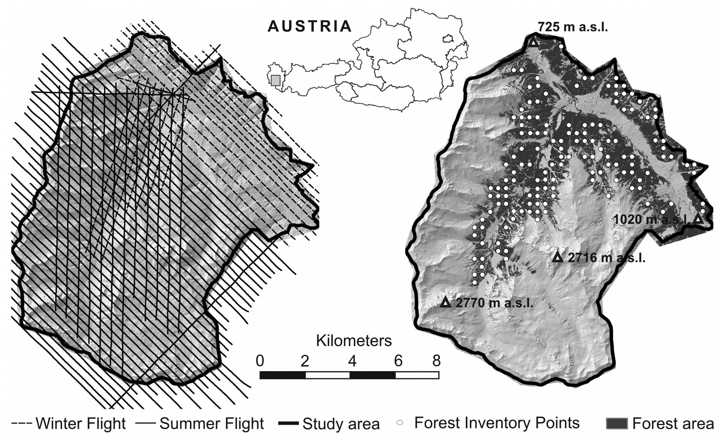
Figure 2.
a) Co-registration of the FI sample plots to the ALS data. The center coordinates of each sample plot have been adapted, that the measured single tree positions fit best to the visually detectable tree positions in the ALS canopy height model and that the measured tree height fit best to the height extracted from the canopy height model. b) Distribution of distances of all 925 measured single trees from 103 FI sample plot centers.

Figure 3.
Scatter plots of stem volumes from ALS data versus forest inventory data. The analyses were based on the 52 forest inventory sample plots covered by the winter and the summer ALS data.
Figure 3.
Scatter plots of stem volumes from ALS data versus forest inventory data. The analyses were based on the 52 forest inventory sample plots covered by the winter and the summer ALS data.

Table 1.
Summary of forest inventory data. The calculations of the shown values are based on mean values per plot as well as on parameters measured on single trees. The statistics are calculated from all available forest inventory plots and only from those plots which could clearly be co-registered to the ALS data. The shown statistics of the winter (W), summer (S) and winter & summer (W&S) data are based on the co-registered sample plots.
| Variable | Data | MIN | MAX | MEAN | SD |
|---|---|---|---|---|---|
| Diameter at breast height [cm] | All: 1,373 trees | 10.0 | 127.0 | 48.2 | 18.5 |
| Co-registered: 925 trees | 10.0 | 127.0 | 47.6 | 18.8 | |
| - W: 853 trees | 10.0 | 127.0 | 46.8 | 18.9 | |
| - S: 559 trees | 10.0 | 127.0 | 51.1 | 18.8 | |
| -W&S: 485 trees | 10.0 | 127.0 | 50.0 | 19.1 | |
| Tree height [m] | All: 1,373 trees | 5.4 | 43.8 | 27.7 | 6.8 |
| Co-registered: 925 trees | 5.4 | 42.2 | 27.0 | 6.8 | |
| - W: 853 trees | 5.4 | 42.2 | 27.1 | 7.0 | |
| - S: 559 trees | 7.0 | 42.2 | 27.7 | 6.6 | |
| -W&S: 485 trees | 7.0 | 42.2 | 28.1 | 6.8 | |
| Number of trees per plot | All: 143 plots | 1 | 29 | 9.8 | 5.4 |
| Co-registered: 103 plots | 1 | 22 | 8.8 | 4.6 | |
| - W: 92 plots | 1 | 22 | 9.3 | 4.6 | |
| - S: 64 plots | 1 | 22 | 8.7 | 4.3 | |
| -W&S: 52 plots | 1 | 22 | 9.3 | 4.4 | |
| Number of trees per ha | All: 143 plots | 8 | 1,876 | 414 | 392 |
| Co-registered: 103 plots | 11 | 1,876 | 393 | 395 | |
| - W: 92 plots | 11 | 1,876 | 429 | 406 | |
| - S: 64 plots | 11 | 1,602 | 309 | 316 | |
| -W&S: 52 plots | 18 | 1,602 | 352 | 335 | |
| Mean diameter at breast height per plot [cm] | All: 143 plots | 11.0 | 78.0 | 49.0 | 14.0 |
| Co-registered: 103 plots | 11.0 | 77.3 | 48.5 | 14.1 | |
| - W: 92 plots | 11.0 | 77.3 | 47.7 | 14.3 | |
| - S: 64 plots | 21.0 | 77.3 | 51.9 | 13.6 | |
| -W&S: 52 plots | 21.0 | 77.3 | 51.3 | 13.9 | |
| Mean tree height per plot [cm] | All: 143 plots | 6.0 | 42.1 | 26.9 | 6.5 |
| Co-registered: 103 plots | 9.5 | 38.6 | 26.2 | 6.4 | |
| - W: 92 plots | 9.5 | 38.6 | 26.6 | 6.5 | |
| - S: 64 plots | 11.3 | 38.0 | 27.1 | 6.1 | |
| -W&S: 52 plots | 11.3 | 38.0 | 27.7 | 6.2 | |
| Calculated stem volume [m3 ha-1] | All: 143 plots | 10.7 | 1,398.0 | 472.8 | 293.8 |
| Co-registered: 103 plots | 15.7 | 1,137.7 | 423.4 | 239.0 | |
| - W: 92 plots | 15.7 | 1,137.7 | 440.2 | 241.9 | |
| - S: 64 plots | 23.0 | 1,137.7 | 415.9 | 230.0 | |
| -W&S: 52 plots | 27.0 | 1,137.7 | 446,6 | 231.9 | |
Table 2.
Evaluation of the appropriate sample plot size. Shown are the final models, the condition numbers (κ), the bias correction factors (RE), the coefficients of determinations (R2), the root mean square errors (RMSE) between estimated and ground reference values and the results of the cross-validation (MIN, MAX, MEAN, and SD) for each sample plot size. The calculations were done using all (103) sample plots.
| Sample plot size | Parameter | |||||||
|---|---|---|---|---|---|---|---|---|
| κ | RE | R2 | RMSE [m3ha−1] | Cross-validation [m3ha−1] | ||||
| MIN | MAX | MEAN | SD | |||||
| Ø18 m | lnvstem,fi = 4.861837 - 0.419251 lnh10,l + 0.857076 lnd6,f - 0.123035 lnd9,l | |||||||
| 19.9 | 1.025544 | 0.84* | 0.354* | -1.151* | 1.442* | 0.000* | 0.376* | |
| 0.83** | 101.4** | -253.1** | 267.1** | 0.0** | 104.0** | |||
| Ø20 m | lnvstem,fi = 3.178314 - 0.027323 lnd2,f + 0.262734 lnd7,f + 0.526734 lnd6,l | |||||||
| 29.0 | 1.039258 | 0.81* | 0.379* | -1.612* | 1.397* | 0.001* | 0.410* | |
| 0.82** | 101.5** | -264.9** | 291.0** | -0.1** | 105.0** | |||
| Ø22 m | lnvstem,fi = 3.090095 - 0.031669 lnd,2f + 0.609494 lnd6,f + 0.204359 lnd7,l | |||||||
| 29.0 | 1.033626 | 0.83* | 0.361* | -1.794* | 1.088* | 0.001* | 0.385* | |
| 0.83** | 99.1** | -255.2** | 272.3** | 0.0** | 102.1** | |||
| Ø24 m | lnvstem,fi = 4.662327 - 0.901615 lnh0,f + 0.523643 lnh30,l + 0.812855 lnd6,f | |||||||
| 27.2 | 1.017166 | 0.85* | 0.343* | -1.773* | 0.936* | -0.002* | 0.365* | |
| 0.84** | 96.8** | -254.7** | 204.1** | -0.3** | 100.0** | |||
| Ø26 m | lnvstem,fi = 4.662327 - 0.901615 lnh0,l + 0.523643 lnh40,l + 0.812855 lnd6,f | |||||||
| 24.5 | 1.019927 | 0.84* | 0.355* | -1.908* | 0.767* | -0.001* | 0.375* | |
| 0.82** | 103.9** | -338.4** | 282.1** | -0.3** | 107.5** | |||
*The values are calculated in the logarithmic scale. The quantities in the logarithmic scale are dimensionless.
**The values are calculated in the arithmetic scale. The bias was corrected using a ratio estimator [34].
Table 3.
Effects of different ALS densities and acquisition times. Shown are the derived coefficients of determinations (R2), the root mean square errors (RMSE) between estimated and ground reference values and the condition numbers (κ). Furthermore, the statistics of the residuals (MIN, MAX, MEAN, and SD) derived from the cross-validation are shown. The calculations were done using all (A), the winter (W), the summer (S), and the winter & summer (W&S) data corresponding to 103, 92, 64, and 52 sample plots. The calculations were done based on the original ALS points and on the thinned (percentage of thinning was 66%; data sets.
| Time | κ | CF | R2 | RMSE [m3ha−1] | Cross-validation [m3ha-1] | |||||
|---|---|---|---|---|---|---|---|---|---|---|
| MIN | MAX | MEAN | SD | |||||||
| Percentage of thinning: 0% | ||||||||||
| A | lnvstem,fi = 4.662327 - 0.901615 lnh0,f + 0.523643 lnh30,l + 0.812855 lnd6,f | |||||||||
| 27.2 | 1.017166 | 0.91* | 0.343* | -1.773* | 0.936* | -0.002* | 0.365* | |||
| 0.84** | 96.8** | -254.7** | 204.1** | -0.3** | 100.0** | |||||
| W | lnvstem,fi = 5.621786 - 1.120663 lnh0,f + 0.553731 lnd4,f + 0.761191 lnd6,f | |||||||||
| 19.7 | 1.012892 | 0.84* | 0.351* | -1.290* | 0.949* | -0.004* | 0.379* | |||
| 0.81** | 110.4** | -249.2** | 300.5** | -0.4** | 114.8** | |||||
| S | lnvstem,fi = 2.955974 + 0.102221 lnh90,f - 0.001293 lnd3,l + 0.729716 lnd6,l + 0.099115 lnhcv,l | |||||||||
| 21.7 | 1.046855 | 0.76* | 0.410* | -2.128* | 0.719* | 0.001* | 0.445* | |||
| 0.82** | 97.9** | -385.7** | 317.5** | 0.8** | 110.7** | |||||
| W&S | W | lnvstem,fi = 4.824553 - 0.399229 lnh0,f + 0.094519 lnh80,f - 0.012827 lnd2,f + 0.696564 lnd6,f | ||||||||
| 20.3 | 1.021042 | 0.81* | 0.327* | -1.097* | 1.134* | 0.006* | 0.384* | |||
| 0.79** | 108.2** | -224.7** | 332.0** | 1.6** | 120.0** | |||||
| S | lnvstem,fi = 3.892341 - 0.217090 lnh0,f + 0.047210 lnh80,f + 0.775024 lnd6,f | |||||||||
| 14.9 | 1.018094 | 0.89* | 0.248* | -0.887* | 0.607* | -0.002* | 0.273* | |||
| 0.85** | 90.9** | -242.1** | 258.9** | -0.6** | 97.2** | |||||
| Percentage of thinning: 66% | ||||||||||
| A | lnvstem,fi = 2.818110 - 0.074578 lnd0,f + 0.282504 lnd7,f + 0.606238 lnd6,l | |||||||||
| 24.5 | 1.026639 | 0.84* | 0.356* | -1.7996* | 0.968* | 0.000* | 0.375* | |||
| 0.82** | 104.4** | -268.5** | 311.9** | -0.1** | 106.7** | |||||
| W | lnvstem,fi = 2.960790 - 0.035852 lnd2,l + 0.610804 lnd6,l + 0.270893 lnd8,l | |||||||||
| 18.6 | 1.025183 | 0.80* | 0.387* | -1.514* | 1.795* | -0.001* | 0.411* | |||
| 0.77** | 117.5** | -297.7** | 410.2** | -0.2** | 122.7** | |||||
| S | lnvstem,fi = 3.124630 + 0.129229 lnh90,f + 0.014617 lnd3,l + 0.682713 lnd6,l + 0.065367 lnhcv,l | |||||||||
| 21.7 | 1.048572 | 0.74* | 0.425* | -2.092* | 1.051* | 0.000* | 0.460* | |||
| 0.82** | 99.9** | -370.9** | 309.2** | 0.2** | 111.3** | |||||
| W&S | W | lnvstem,fi = 3.472091 + 0.295300 lnh0,f - 0.510809 lnh30,f + 0.589993 lnh70,f - 0.098405 lnd2,f + 0.483818 lnd6,f | ||||||||
| 28.3 | 1.021042 | 0.80* | 0.333* | -1.259* | 1.047* | 0.003* | 0.402* | |||
| 0.77** | 113.3** | -304.0** | 317.0** | 0.0** | 127.1** | |||||
| S | lnvstem,fi = 2.925126 + 0.250145 lnh0,f + 0.492056 lnh80,f - 0.148622 lnd2,f + 0.353557 lnd5,f | |||||||||
| 25.8 | 1.010784 | 0.85* | 0.293* | -1.251* | 0.940* | -0.011* | 0.363* | |||
| 0.85** | 93.3** | -276.4** | 282.0** | -2.4** | 104.0** | |||||
*The values are calculated in the logarithmic scale. The quantities in the logarithmic scale are dimensionless.
**The values are calculated in the arithmetic scale. The bias was corrected using a ratio estimator [34].
© 2007 by MDPI ( http://www.mdpi.org). Reproduction is permitted for noncommercial purpose.
Share and Cite
MDPI and ACS Style
Hollaus, M.; Wagner, W.; Maier, B.; Schadauer, K. Airborne Laser Scanning of Forest Stem Volume in a Mountainous Environment. Sensors 2007, 7, 1559-1577. https://doi.org/10.3390/s7081559
AMA Style
Hollaus M, Wagner W, Maier B, Schadauer K. Airborne Laser Scanning of Forest Stem Volume in a Mountainous Environment. Sensors. 2007; 7(8):1559-1577. https://doi.org/10.3390/s7081559
Chicago/Turabian StyleHollaus, Markus, Wolfgang Wagner, Bernhard Maier, and Klemens Schadauer. 2007. "Airborne Laser Scanning of Forest Stem Volume in a Mountainous Environment" Sensors 7, no. 8: 1559-1577. https://doi.org/10.3390/s7081559