Energy-efficient Optimization of Reorganization-Enabled Wireless Sensor Networks

State Key Laboratory of Precision Measurement Technology and Instruments, Tsinghua University, Beijing 100084, P. R. China
*
Author to whom correspondence should be addressed.
Sensors 2007, 7(9), 1793-1816; https://doi.org/10.3390/s7091793
Submission received: 9 August 2007
/
Accepted: 4 September 2007
/
Published: 5 September 2007
(This article belongs to the Special Issue Energy Efficiency and Intelligent Signal Processing for Wireless Sensing)
Abstract
:This paper studies the target tracking problem in wireless sensor networks where sensor nodes are deployed randomly. To achieve tracking accuracy constrained by energy consumption, an energy-efficient optimization approach that enables reorganization of wireless sensor networks is proposed. The approach includes three phases which are related to prediction, localization and recovery, respectively. A particle filter algorithm is implemented on the sink node to forecast the future movement of the target in the first prediction phase. Upon the completion of this phase, the most energy efficient sensor nodes are awakened to collaboratively locate the target. Energy efficiency is evaluated by the ratio of mutual information to energy consumption. The recovery phase is needed to improve the robustness of the approach. It is performed when the target is missed because of the incorrect predicted target location. In order to recapture the target by awakening additional sensor nodes as few as possible, a genetic-algorithm-based mechanism is introduced to cover the recovery area. We show that the proposed approach has excellent tracking performance. Moreover, it can efficiently reduce energy consumption, prolong network lifetime and reduce network overheads.
1. Introduction
Wireless sensor networks (WSNs) consist of many randomly deployed wireless sensor nodes, which have the ability to sense the environment, process the information and disseminate data wirelessly. A sink node, which has relative powerful computing and communication capacity, is located in WSN for processing and exchanging data. Due to the inherent limitations of sensor nodes such as small sensing scope, low sensing precision and scanty energy resource, sensor nodes should collaboratively measure a target constrained by energy consumption. Most sensor nodes provide four different modes for radio transmission: transmit, receive, idle and sleep. To conserve precious energy resource, sensor nodes keep sleeping most of the time. The fewer sensor nodes are awakened, the less energy is consumed. Therefore, sensing optimization is an important issue in WSN and approaches are introduced to settle this problem [1]. In this paper, we study sensing optimization strategies for target tracking in WSN. The problem is complicated because detection quality, tracking quality and energy consumption are critical metrics [2].
To track a moving target, it needs to detect the presence of the target first. With prediction-based approaches, the number of awakened sensor nodes for detection can be sharply reduced. In [3-5], it is assumed that sensor node observations are accurate and each sensor node can get the perfect target location independently once the target moves into its sensing range. This assumption makes the problem easy because the tracking results are only relative to the detection results. In fact, sensor node observation error is an important parameter which can affect prediction error and tracking accuracy. In [6], the authors take account of the sensor node observation error and study a more realistic target motion model. But the work doesn't pay attention to dealing with the missing targets, so that the proposed approach isn't robust enough.
With the prediction results, the network alerts appropriate sensor nodes to locate the target in the next tracking period. Because of the collaborative essence, sensor node selection is a critical issue for saving energy [2, 7-9]. In [2], the authors propose the information-driven sensor querying (IDSQ) approach, where the selected sensor nodes can collaboratively increase target location information with low communication energy consumption. Time efficiency is not considered in the work and the approach is also not energy efficient enough. If the selected sensor node can't detect the target, the target location information is still transmitted to the sensor node which causes extra energy waste. The approaches in [2] and [7] are damageable as no mechanism to recovery from target missing.
Because of the uncertainty of target mobility and sensor node detection ability, blind sensor node may appear during collaborative target location [10]. Especially when the first selected sensor node can't detect the target, none of the target location information can be gained, which implies that the target totally missed in this tracking period. In that case, the network needs to be reorganized to capture the target. Network reorganization increases target searching area by awakening extra sleeping sensor nodes. In [3, 5], the network first awakens all neighbor sensor nodes around the current sensor node. If the target still can't be found, all the sensor nodes in the network are awakened. This process can guarantee a large probability to find the target, but it's not energy efficient enough. In [10], a geometric method is introduced. It's fast, but not practicable if the sensor node detection ability is uncertain.
In this paper, we propose an energy-efficient optimization approach that enables reorganization of WSN. The proposed approach contains three phases: prediction phase, localization phase and recovery phase. The sink node performs particle filter to predict target trajectory and awakens the sensor node nearest to the predicted result. In the localization phase, the most energy-efficient sensor node is selected to apply a measurement and update target distribution in each step. Energy efficiency optimization and time efficiency are both considered in the sensor node selection. To improve the robustness of the approach, a recovery mechanism is performed to find the target again in case that the selected senor node can't detect the target. Sensor node selection for recovery is based on a pre-performed genetic algorithm (GA). We show that the proposed approach is energy-efficient and can prolong the lifetime of WSN.
The rest of the paper is organized as follows: Section 2 provides system architecture and basic models of WSN for later analysis. In Section 3, we present the details of our approach, including prediction phase, localization phase and recovery phase. In Section 4, experimental results are presented to evaluate the performance of the proposed approach. Finally, the conclusion is given in Section 5.
2. Target Tracking in Wireless Sensor Network
In this section, we describe the system architecture of target tracking in wireless sensor network, and set up assumptions on basic models for illustration and later analysis, including bearing sensor node detection model, observation and collaboration model, energy consumption model and linear target motion model.
2.1. System architecture
Here, we assume that stationary sensor nodes are uniformly distributed in the sensing field. All of the sensor nodes have four different radio modes: transmit, receive, idle and sleep. Sleep mode consumes the least power compared with other modes. To support sleep mode, a low power paging channel in the physic layer, which keeps running at full duty, is used to communicate among sensor nodes [11]. Through this low-power paging channel, a sensor node can be awakened by other sensor node or by the sink node. Each sensor node can determine its location by exploiting Global Position System (GPS). Sensor nodes report the information about themselves (such as locations) to the sink node periodically. The sensor node broadcasts the information to the network and makes each one receive the whole network knowledge. With power control technology, sensor nodes can change communication range in order to reduce radio energy consumption and improve connectivity [12]. For each sensor node, any other sensor nodes in its communication range could become its neighborhoods. Due to the limited transmission ability of sensor nodes, data transmission is usually multi-hop (from a sensor node to another sensor node, towards to the sink node). The sink node has relatively powerful transmission capacity. It can send data to any sensor nodes in the network directly, if the sensing field is not very large.
2.2. Sensor node probability detection model
Because wireless sensor nodes have limited sensing range, a sensor node could monitor a target only when the target moves into its detection range. Binary detection model and probability model are both presented to describe detection capacity of sensor nodes [13, 14]. In fact, sensor node detections can be easily affected by environmental noise. The detection result is uncertain, especially when the target is near the edge of the detection range where the signal-noise-ratio (SNR) is small. In order to describe the uncertainty of sensor node detections, we assume a probability model in this paper. The probability of point q detected by sensor node si is given as below:
where the superscript d of
denotes detection, and the subscripts x,y denote the coordinates of point q; r is the dete]ction range; re is the detection uncertainty range;d(si, q) is the Euclidean distance between sensor node si and the point q; λ, β1, β2 are parameters of the detection model; α1=re−r+d(si,q) and α2=re+r−d(si,q). Figure 1 shows detection probabilities with different d(si,q). It is assumed that the detection range is unit and the range of detection error is 0.4 units. Different from binary detection model, probability model doesn't have a step change, so it's more realistic to describe detection capacity of sensor nodes.
If point q can be detected by several sensor nodes, the collaborative detection probability is:
where Sov is the set of detectable sensor nodes. We define that a point can be detected efficiently if
where
is the efficient detection threshold.
2.3. Observation and collaboration model
In WSN, targets are present in a location domain. The goal of tracking is to locate the target to some accuracy in each tracking period. As a single sensor node is accuracy-limited, aggregating sensor node observations is generally used to improve tracking accuracy. It is assumed that bearing sensor nodes are randomly scattered in the network. Let (xtar,ytar) and (xs,ys) denote the target location and sensor node location, respectively. The bearing sensor node observation is [15]:
where w1 is the perturbation noise, which can be simplified as zero mean Gaussian noise.
Aggregating sensor node observations can reduce the target location distribution error. With Bayesian estimation, sensor node observations can be fused step by step [8, 16]. Denote target location random and its realization value by X and x, respectively. Let Zi and zi denote the ith awakened sensor node observation random and its realization value, respectively. The posterior target location distribution incorporated with the jth awakened sensor node observation is [8]:
where C is a normalization constant. If sensor node observations are conditionally independent with each other conditioned on target location, Equation (5) can be expressed as below for short.
We use root-mean-square-error (RMSE) to measure the target location distribution estimation error
where x̄ is the true value of target location; E(·) is the expectation of target location distribution p(x|z1,…,zj); ‖·‖ is the Euclidean distance. As the true target location x̄ is actually unknown, we use E(x) to approximate it.
2.4. Sensor node energy consumption model
A wireless bearing sensor node consists of several components, including MCU (micro control unit), radio, sensors and memory. Each component consumes different amounts of power in different modes. Table 1 shows the basic energy consumption of different components.
Here, PT and PR denote the transmission power and receiving power, respectively. Their values are relative to the characteristics of the radio [17]. It is assumed that energy consumed by transmitting a k bit packet d distance is:
where Ete is the transmitter circuitry energy; εamp is the transmit amplifier energy; □tT(k) is the time for transmitting k bit data. To receive the same packet, a sensor node should cost energy ER:
where Ere is the receiver circuitry energy; □tR(k) is the time for receiving k bit data; □tT(k) and □tR(k) are determined by radio transmission rate. Values of these parameters are shown in Table 2.
2.5. Linear target motion model
In our approach, the sink node predicts target movement according to the target motion model. For the ground target tracking applications in a 2-dimensional domain, the state vector of the moving target can be expressed as below:
where (xt,yt) is the target location at time t and (ẋt,ẏt) is the target velocity at time t.
For linear cases, target state transition function can be expressed by [18]:
where F is the state transition matrix; Vt is the process noise at time t; G is the process noise matrix. Given the target tracking period T, the expressions of F and G are given as below:
3. Optimal Strategies for Target Tracking Sensing
Based on the system architecture and basic models, an energy-efficient optimization approach that enables reorganization of WSN is presented in this section. The basic idea of the approach is to reduce the number of awakened sensor nodes.
3.1. Target motion prediction phase
In a target tracking network, sensor nodes collaboratively locate the target and then report the results to the sink node. Hence, the sink node keeps the whole information about the tracked target. It is assumed that if there is no target in the sensing field, some sensor nodes are still awakened periodically to keep enough coverage of the sensing field. When a target moves into the sensing field, it can be detected, located and reported to the sink node by some active sensor nodes. When the initial information about the target is enough, the sink node has the ability to anticipate the future movement of the target and activate the sensor nodes necessary to monitor it.
The sink node has the capacity to implement some dense computing prediction algorithm. Here, we propose the particle filter algorithm for prediction. The particle filter is a nonparametric method. It is well suited to the target tracking problem in WSNs, where target distributions may be non-Gaussian.
Basic steps of particle filter algorithm is given as below [19-21]:
- 1)
- Initialize particles and importance weights.Particles are initialized to satisfy the prior distribution. Importance weights of the ith particle in the kth step prediction are initialized to bewhere Ns is the number of particles.
- 2)
- Update particles and importance weightsParticles are updated to bewhere i = 1, …, Ns; is the predicted target state of the ith particle in the kth step;F and G are defined in Section 2.5.With sensor node observations, importance weights are updated to bewhere p(·) and q(·) are both conditional probabilities.Then, importance weights should be normalized to be
- 3)
- Resample particlesIt is defined that efficient sample size is:where is derived from residual resampling. If Neff is less than the theoretical threshold, particles should be resampled with importance weights .
- 4)
- Update target stateWhere χk is the updated target state in the kth step.
The predicted target location in the kth step can be derived from Equation (14):
where
is the location part of
.
In the tracking applications, the model of target motion is uncertain. The collaborative localization is also accuracy-limited. These two factors both make the system model incorrect, which brings considerable prediction error [22].
3.2. Collaborative target localization phase
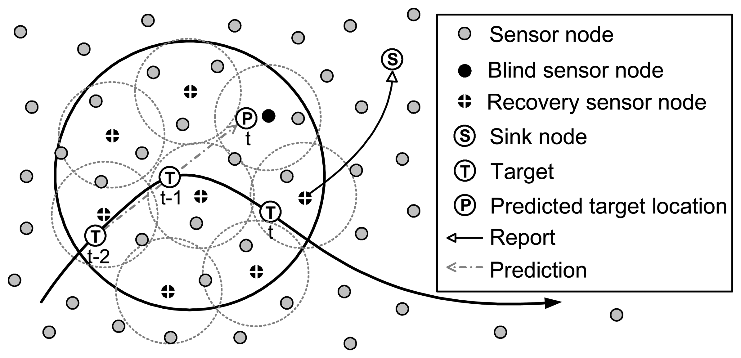
When the prediction phase is finished, a localization phase is performed to select sensor nodes for collaborative localization. The collaborative target localization phase is analogous with the IDSQ proposed in [2]. But we pay more attention to the time constraint and energy efficiency, and a mechanism dealing with the missing target is contained in this phase, which makes our approach robust enough. Figure 2 displays the localization scenario. Firstly, the sink node awakens a sensor node to monitor the target according to the predicted target location. The active sensor node, also called the predicted sensor node, collects the target information and produces a target location distribution. Then, it activates another sensor node for observation by some metrics. For simplicity, we call the sensor node performing selection designator and the selected sensor node designee. The designee applies a measurement to the target. A “Yes” message is sent to the designator if the designee detects the target and a “No” message if not. When the designator receives a “Yes” massage, it transmits the target location distribution to the designee and then goes back to sleep. The designee then becomes a new designator. It updates the target location distribution and awakens another sensor node. By repeatedly awakening a new sensor node to monitor the target, the uncertainty of target location distribution reduces. Collaboration stops when termination conditions are satisfied. At last, the current designator reports the collaboration result to the sink node and a tracking period finishes.
From the information-theoretic point of view, sensor node observations increase the information about the target. The goal of sensor node selection is to find the most energy-effective sensor node in each step so as to prolong the life-time of the network. As sensor node selection implies data transmission, the objective function for sensor node selection should be a combination of information gain and energy consumption. It can be defined as:
where φjinf is the information gained by sensor node observation, ψcost is the energy consumption. Thus, the selected sensor node i should satisfy:
where S is the set of candidate sensor nodes. It can be defined as:
where N is the number of sensor nodes in the network; ‖·‖ is the Euclidian distance; r+re is the maximal detection range; xi is the location of sensor node i; x̄ is the true target location which is unknown actually. Here, we use E(x) to approximate x̄.
How to evaluate the expected information gain before sensor node observation is the core problem of sensor node selection. In previous works, the notion of mutual information was introduced [23, 24]. The mutual information I(X,Zi) between the target location random X and the predicted sensor node observation random Zi is:
According to Section 2.4, if sensor node i awakens sensor node j, it should cost
where αp,q represents the reliability of the transmission between sensor node p and sensor node q,αp,q∈ [0,1]; k; is the data needed to be transmitted; Ec is the energy consumed to awaken a sensor node; l is the shortest routing from sensor node i to sensor node j. As each sensor node knows any others' positions, the shortest routing between two sensor nodes can be calculated by the Dijkstra algorithm [25]. Thus, Equation (21) can be expressed as:
At the beginning of each tracking period, there is no prior target distribution. It is assumed that each sensor node has the same mutual information. Because the energy consumed by the sink node can be ignored, Equation (25) can be simplified as
where xi denotes location of sensor node i; x̂ is the predicted target location.
As sensor nodes are randomly scattered, it's possible that several sensor nodes have the same distance to the predicted target location. If so, the one closest to the sink node is selected.
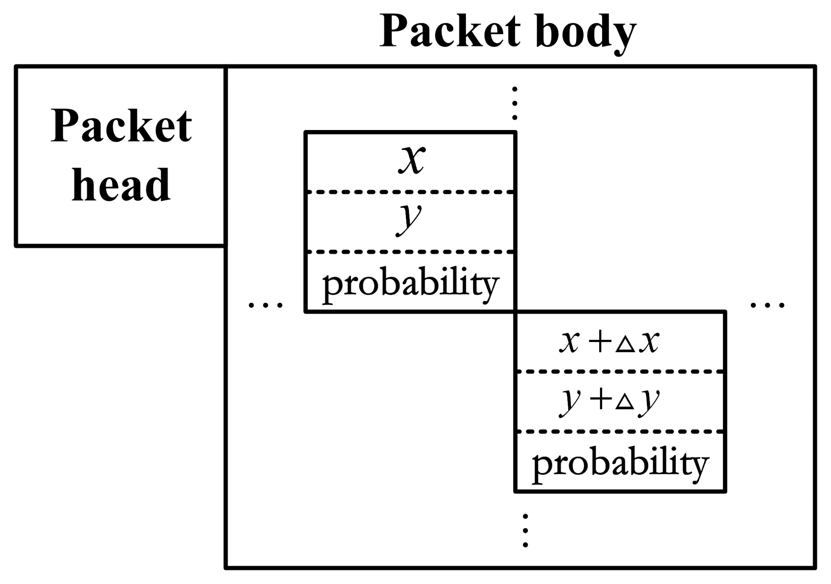
The selected sensor node needs to update the target distribution by its measurement and prior distribution. The whole packet transmitted is defined in Figure 3, where □x and □y is the grid size of target location distribution. Packet head contains source and destination IDs, packet size and other useful information. It is small enough to be ignored compared with the packet body. The grid size of target distribution affects localization precision, which is determined by application.
Obviously, transmitting the whole information about the target location distribution may augment packet size and waste energy. We set a transmission probability threshold
to decide whether the point information should be transmitted. Let
denote the probability of target location distribution at point (x,y). The information transmission probability
of point (x,y) can be expressed as:
where
is the collaborative detection probability computed by Equation (2).
As the probability model is introduced to describe sensor node detection capacity (see Section 2.2), there's a problem with what to do if an active sensor node can't detect the target. Because environmental impacts always change slowly, the sensor node may remain blind to the target for a while. Thus, using a sensor node to observe successively is impossible to improve detection probability. If the blind sensor node is also the predicted sensor node, a recovery mechanism proposed below is performed to find the target. If a blind sensor node appears during the collaboration procedure, a simple method is then used. Obviously, when a designator wants to select a sensor node, it needs to compute Equation (20) for all of the candidate sensor nodes. In case that the optimal sensor node misses the target, the designator could awaken the sub optimal sensor node. If the target still can't be detected, the less optimal sensor node is designated. Thus, the detected probability of the target can be greatly improved. To avoid awakening too many sensor nodes, which is a waste of time, it is assumed that the awakening steps can't be more than a constant number Na, whose value is determined by the maximum speed the network can track and the allowed upper bound of the target localization error.
Collaboration stops in three cases. 1) The predefined target localization accuracy is satisfied. 2) All candidate sensor nodes have been awakened. To avoid some sensor nodes depleting energy too fast, which shortens the lifetime of the network, a heuristic is proposed that each sensor node can only be awakened no more than one time in a single tracking period. 3) Awakening steps is larger than Na. It defines that the target is In when the collaboration stops in case 1 and Out when the collaboration stops in case 2 or 3.
3.3. Recovery phase for tracking failure
Considering the unpredictable behavior of the target and the uncertainty of the sensor node detection ability, it is impossible to guarantee a 100% probability that the predicted sensor node can detect the target. The whole tracking process may be interrupted just because the target is missed in a tracking period. To avoid these situations, a recovery mechanism is necessary to recapture the target.
The essential of recovery mechanism is to increase the coverage by awakening extra sleeping sensor nodes. While the coverage is satisfied, the number of the awakened sensor nodes should be as few as possible. Thus, it also can be defined as a local coverage optimization problem. As detection probability model is introduced in Section 2.2, it's impossible to use geometric method [10] to estimate coverage rate. However, the problem can be easily settled by genetic algorithm (GA). GA is a traditional evolution algorithm which is widely used in global search problems. It can get approximate optimal solutions easily, but it converges slowly near the optimal solution. Running GA real-timely during target tracking on the sink node is impossible and unnecessary. In fact, GA optimized result is only relative to the network topology which keeps constant in a fairly long time. Sensor nodes report their information to the sink node periodically, thus the sink node keeps the current topology of the network. It has enough time to perform GA and thus knows which sensor nodes should be awakened to detect at any moment.
Let va denote the maximum target speed the network can track. Let
denote the recovery area at tracking time t.
Recovery mechanism is displayed in Figure 4, where the dashed circle is the detection range and the solid circle denotes the recovery area. When the sink node receives a “No” message, it awakens the sensor nodes around the blind sensor node to cover the recovery area. We call the sensor node selected for recovery mechanism the recovery sensor node. If some recovery sensor nodes find the target, they report to the sink node and the one nearest to the target is designated to be the new designator.
The ideal sensor node selection mechanism for recovery process is that the sensor nodes selected only cover the recovery area. It needs to be done in a real-time manner, which is impossible for GA. Here, we use an approximate approach that contains two steps. First, candidate sensor nodes that can cover the whole sensing field are determined by GA, as proposed in [26]. Second, the useful sensor nodes which can efficiently cover the recovery area are selected.
Using GA to cover the whole sensing field is not difficult. It is assumed that there are N sensor nodes in the network. Let sni denote the state of sensor node i. The value of sni is defined as below:
Thus, the state vector of the whole network can be expressed as:
Obviously, efficient coverage rate and energy consumed to awaken sensor nodes are both crucial metrics to select recovery sensor nodes. In this paper, we define the fitness function of GA for selecting recovery sensor nodes:
where Ce is the efficient coverage rate of the selected sensor nodes; Cr denotes the energy consumed to awaken the selected sensor nodes; f(·) is a function to control the importance weight of coverage rate in optimized solution. For simplicity, we define that the optimal coverage rate should be larger than a threshold cth ∈ (0,1]. The function can be expressed as:
where Cmax is the maximal coverage rate achieved by awakening all sensor nodes in the network.
Efficient coverage rate Ce can be calculated by a grid algorithm
where ne is the number of grids that can be covered efficiently. It is calculated by the sensor node detection model (see Section 2.2); na is the number of all grids. The grid size affects the coverage precision.
Energy consumed for recovery Cr is only relative to the number of the active sensor nodes, that is:
where Ec is the same definition as that in Equation (24).
GA optimization is used to find out the network state vector that has the maximal fitness value. The termination condition of GA is the maximum generation Gm. If Gm is not very large, GA could get several solutions with different initial populations. The solution that can cover the recovery area most energy-efficiently (i.e., has the maximal fitness value, where Cr excludes the energy consumed to awaken the current blind sensor node) is selected.
The recovery mechanism is designed with two steps:
- 1)
- GA_Cover. As we use GA to do global optimization instead of local optimization, the selected sensor nodes located inside the recovery area may not satisfy the coverage rate. In Figure 5, some selected sensor node located outside the recovery area provides a great coverage to the area. It also seems that the farther a sensor node is away from the edge of recovery area, the less it contributes to the coverage of the area. Thus, to simply adapt the recovery sensor node, we define an awakening area with the radius rawhere rr is the radius of the recovery area. It can be calculated as rr =va ·□t + εa; ρ is a adapting coefficient. It is relative to the parameters of the sensor node detection model and varies with sensor node locations.Sensor nodes located inside the awakening area are first awakened to detect the target. The GA Cover step could ensure a nearly maximal probability to recapture the target.
- 2)
- Complement. If the GA_Cover step still can't find the target, a Complement step is performed to cover the left area. This guarantees the maximal probability to find the target.
The recovery phase is efficient only if some sensor nodes can detect the target. If the target falls into a blind spot, no sensor node can detect it. In such cases, though the target can not be located, the recovery process is still performed, because only if the recovery process can't find the target, the sink node can determine that the target is in a blind spot.
4. Experimental Results
Here, we present the results of several experiments to evaluate the performance of our energy-efficient optimal strategies for target tracking sensing.
4.1. Experimental setup
In our experiments, 300 sensor nodes are uniformly distributed in a 300 m × 300 m area. The sink node is located at (150 m, 150 m). Each sensor node has a detection radius of 30 m, and the range of detection error is 12 m. The parameters of the sensor node detection model are λ=1, β1=1, β2=0.5 [used in Equation (1) ]. A point in the sensing field could be efficiently covered only when the detection probability exceeds 0.9. Sensor nodes can directly link to others in the range of 90 m with the reliability α =1. Sensor nodes should keep radio on for 40 ms to ensure data integrity. They also need 30 ms for sampling and computing to reach a conclusion. According to Table 1, the energy consumed to awaken a sensor node is:
The tracking period is determined by the application and it is set to be 2 s. The sensing field is divided into rectangles (1 m × 1 m) and (6 m × 6 m) for target distribution transmission and recovery, respectively. The threshold of transmission probability is set to be
experientially. The network is designed to track vehicles with the maximal velocity less than 30 m/s. In a tracking period, it allows to awaken sensor nodes within Na=5 steps. GA population size is 100. The maximum generation is 100. The probability of crossover and mutation is 0.950 and 0.050, respectively. We set the minimum coverage threshold cth=95.0% to guarantee enough coverage. The recovery range adapting coefficient is set to be ρ =1.1 according to the sensor node locations and parameters of the detection models.
In this paper, a vehicle moves through the sensing field, with a maximum velocity of 20 m/s and a maximum acceleration of 4 m/s2. Figure 6 shows the target tracking scenario. The vehicle moves randomly in the sensing field, and the whole 60 tracking periods are studied.
The experiments consist of two parts. Firstly, tracking procedures are presented to display what happens in our approach. Then, impacts of localization error upper bound εa and sensor node observation standard deviation σ are studied. Energy consumption is used to evaluate the performance of the proposed approach.
4.2. Vehicle tracking procedures
It is assumed that the standard deviation of Gaussian sensor node model is σ =8°. The allowed upper bound of target localization error is εa=4m. When the target moves into the sensing field, some active sensor nodes catch the target and locate it. It is assumed that in the first two tracking periods, the sink node doesn't perform prediction phases because past information of target locations is not enough. In the left 58 tracking periods, prediction errors are studied.
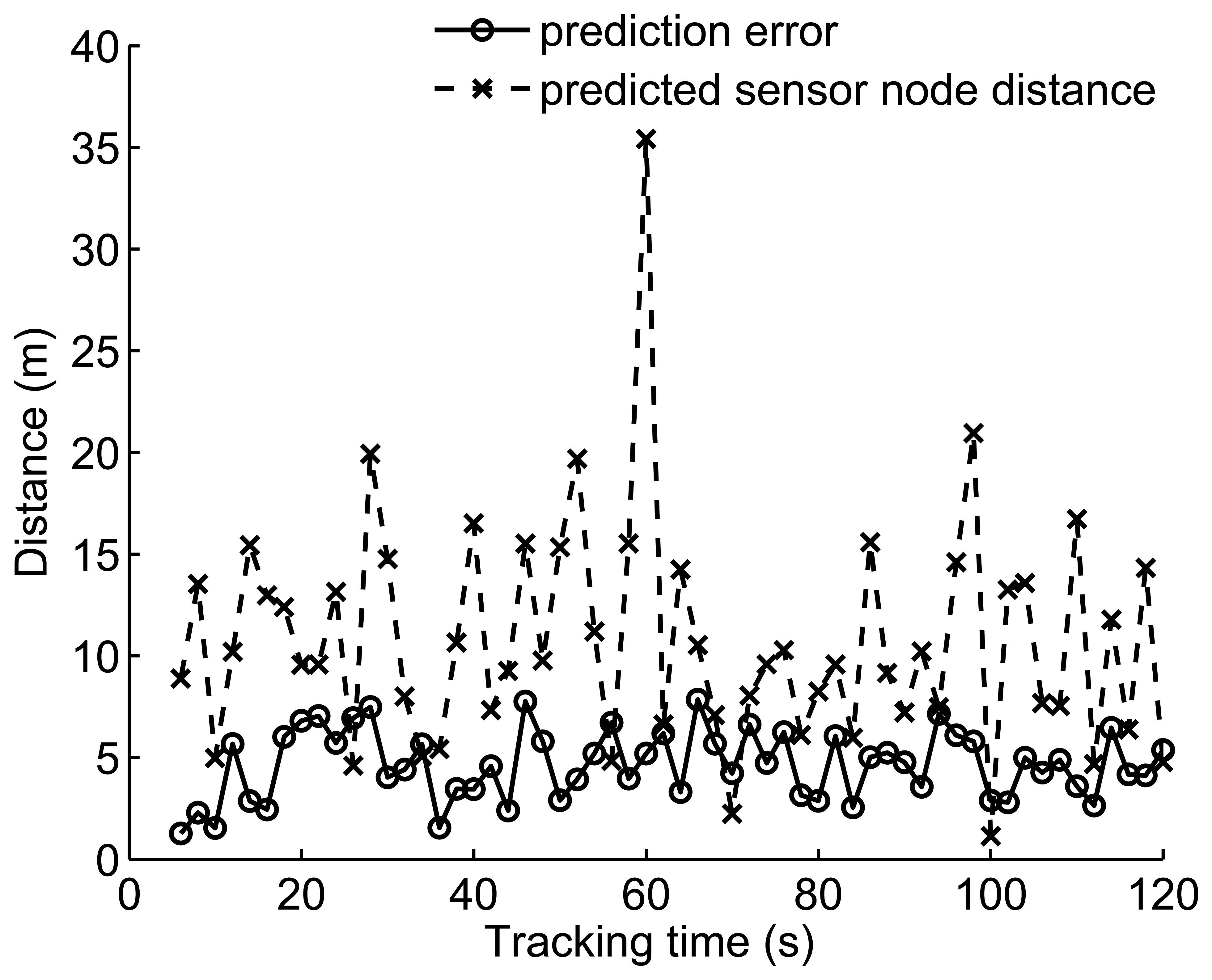
Figure 7 shows the prediction results, which indicate that most of the prediction errors are less than 8 m, with relative errors less than 2.7%. The sensor nodes nearest to the prediction results are awakened and apply measurements to the target. The distance between target and the nearest sensor node determines whether the recovery mechanism is performed. Prediction error and sensor node density are both decisive factors to the distance. Figure 7 indicates that all of the distances are less than 20 m (with the detection probability of 0.972) except at time 60 s. At this instant, the target moves through a sparsely deployed region, and the predicted sensor node distance is more than 35 m (with the detection probability less than 0.003).
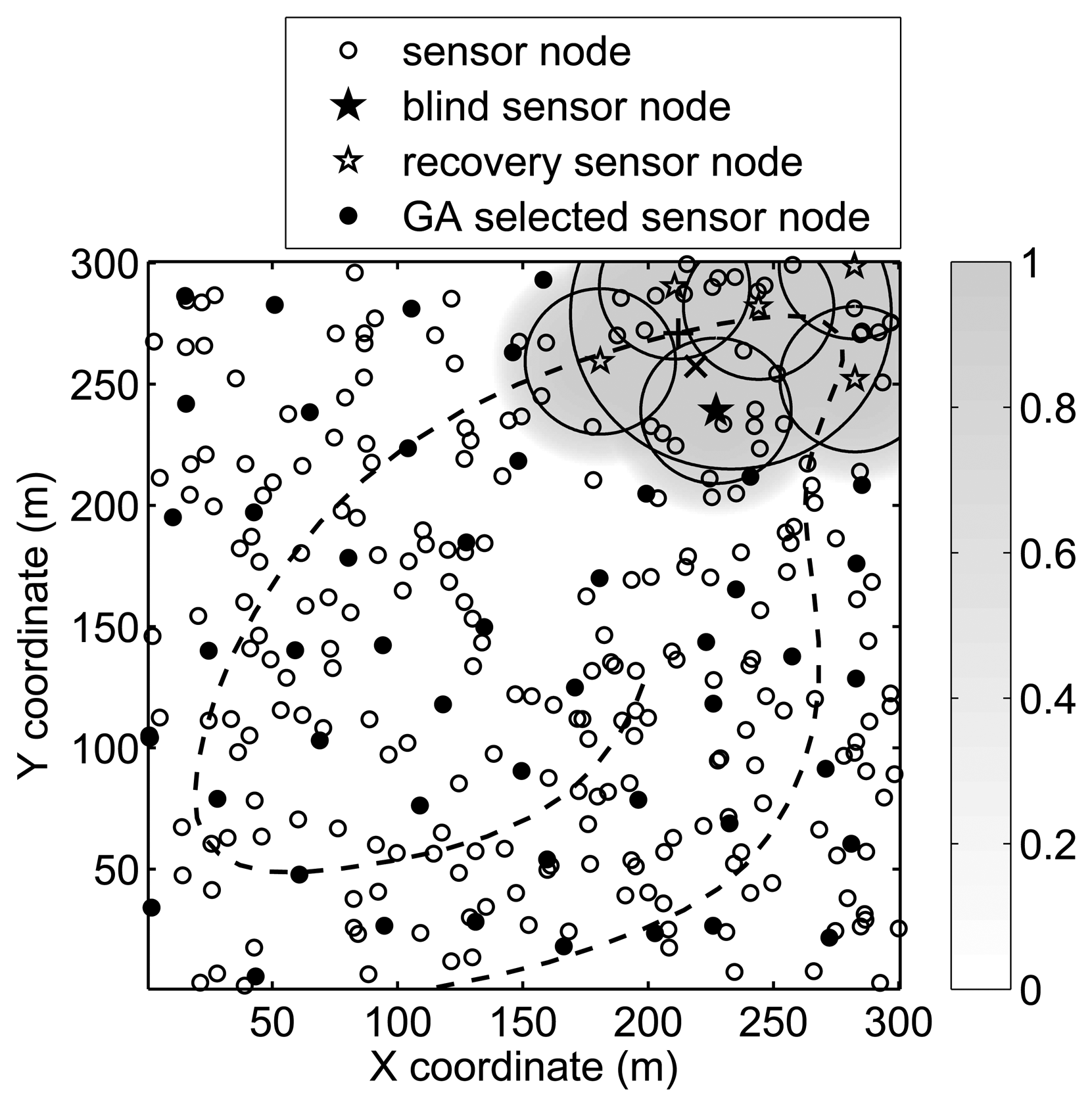
If there's no recovery mechanism, the target would be missed after tracking for 60 s. To avoid this situation, the recovery mechanism is performed to catch the target. Figure 8 displays the recovery procedure, where“+” denotes the true target location and “x” denotes the predicted target location. The thin solid line denotes the sensor node detection range. The thick solid line denotes the awakening range. The dashed line denotes the target trajectory and the grayscale represents the coverage rate. With GA optimization, 53 sensor nodes are selected to cover 96.5% of the whole sensing field. There are 31 sensor nodes located inside the recovery area, and only five of them are awakened to detect the target, which can cover 97.2% of the recovery area.
Tracking accuracy, which is indicated in Figure 9, is the most important metric in the target tracking application. The horizontal solid line in the figure represents the localization error upper bound of 4 m. In most of the tracking periods, localization errors are less than the allowed target localization error upper bound except at time 40 s and 60 s. In fact, tracking accuracy is reactive to the sensor node locations. At time 40 s, the target is located at (235.1 m, 204.9 m), where sensor nodes are scattered sparsely around. Because there are not enough sensor nodes to provide reliable observations, the collaborative localization stops when the awakening steps Na is achieved. At time 60 s, a recovery mechanism is performed, which means an extra step is used to find the target. Thus, there are no enough steps left to locate the target accurately.
Energy consumption in each tracking period is presented in Figure 10, where the energy consumed by communication between sensor nodes and the sink node is ignored. The energy consumption without optimization is calculated by a simple mechanism that can be expressed as below:
- All the sensor nodes located within the range of 24 m around the predicted target location are awakened to detect the target in each tracking period.
- Sensor node measurements are aggregated in a central sensor node. The central sensor node is selected from all the sensor nodes in the range of 24 m, which can minimize the communication energy.
- The range 24 m is the lower bound that the target can be located in each tracking period with the sensor node distribution and target trajectory shown in Figure 6.
The energy consumption with optimization is calculated by our approach. We divide energy with optimization into two parts for analysis. Awakening energy represent the energy consumed to keep sensor nodes active, which is proportional to the awakened sensor node number. Communication energy is determined by the amount of transmitted data and distance. It seems that the energy consumption of our approach is much less than that of the mechanism without optimization in each tracking period except when there is a recovery process. Furthermore, more sensor nodes awakened means more energy consumed for communication.
4.3. Impact of localization error upper bound
Prediction error grows very quickly with an incorrect system model. The upper bound of localization error εa is a crucial parameter in the system model. The value of εa implies the required tracking accuracy and has a great influence on the prediction result. Therefore, it's important to analyze impact of εa on the total energy consumption. In general, the value of εa is determined by applications. Different from other parameters, an application always presents its requirement in the way of “The maximum location error should be no more than”. Thus, there is space to choose an appropriate value to reduce the energy consumption. Here, we assume that the value of εa is allowed to be less than 5% of sensing field. We study the energy consumption of localization and recovery when the value of εa varies from 1 m to 15 m. Energy consumptions are the average of 100 iterations.
Impact of εa is presented in Figure 11. Two parts of energy consumption are analyzed: localization energy, which is computed by Equation (24) and recovery energy, which is derived by Equation (34). It seems that when εa is less than 5 m, the network rarely needs recovery so that only a little energy is consumed for recovery. When the value of εa increases, measured noise in the particle filter rises and results in worse PF prediction results. When the predicted target locations can no longer correctly reflect the true target locations, the frequency of recovery performing increases and more energy is consumed for recovery. When the value of εa is more than 12 m, recovery mechanisms are performed much more frequently, along with the range of recovery area increasing. Both two factors make the recovery energy consumes quickly. However, the energy consumed for localization has the opposite trend. When the value of εa is small, it's hard for sensor nodes to reach the localization accuracy within the maximal awakening steps Na. Therefore, energy consumed for localization keeps high. When the error becomes more than 7 m, in most of the tracking periods, it only needs two active sensor nodes for localization, and the energy for localization keeps low.
The total energy consumption can be computed as:
where Ep, EL and ER denote the energy consumed in the prediction phase, localization phase and recovery phase, respectively. Similar to Figure 10, we ignore the energy consumed by communications between sensor nodes and the sink node. The total energy consumption is:
The total energy consumption with different εa is shown in Figure 12. It seems that the network has the minimal energy cost when the value of εa is set to be 7 m. As it's defined at the end of Section 3.2, the Out target rate is 8.33%. Certainly, if the application requires that the localization error is less than 7m, the energy consumption reduces when the error rises.
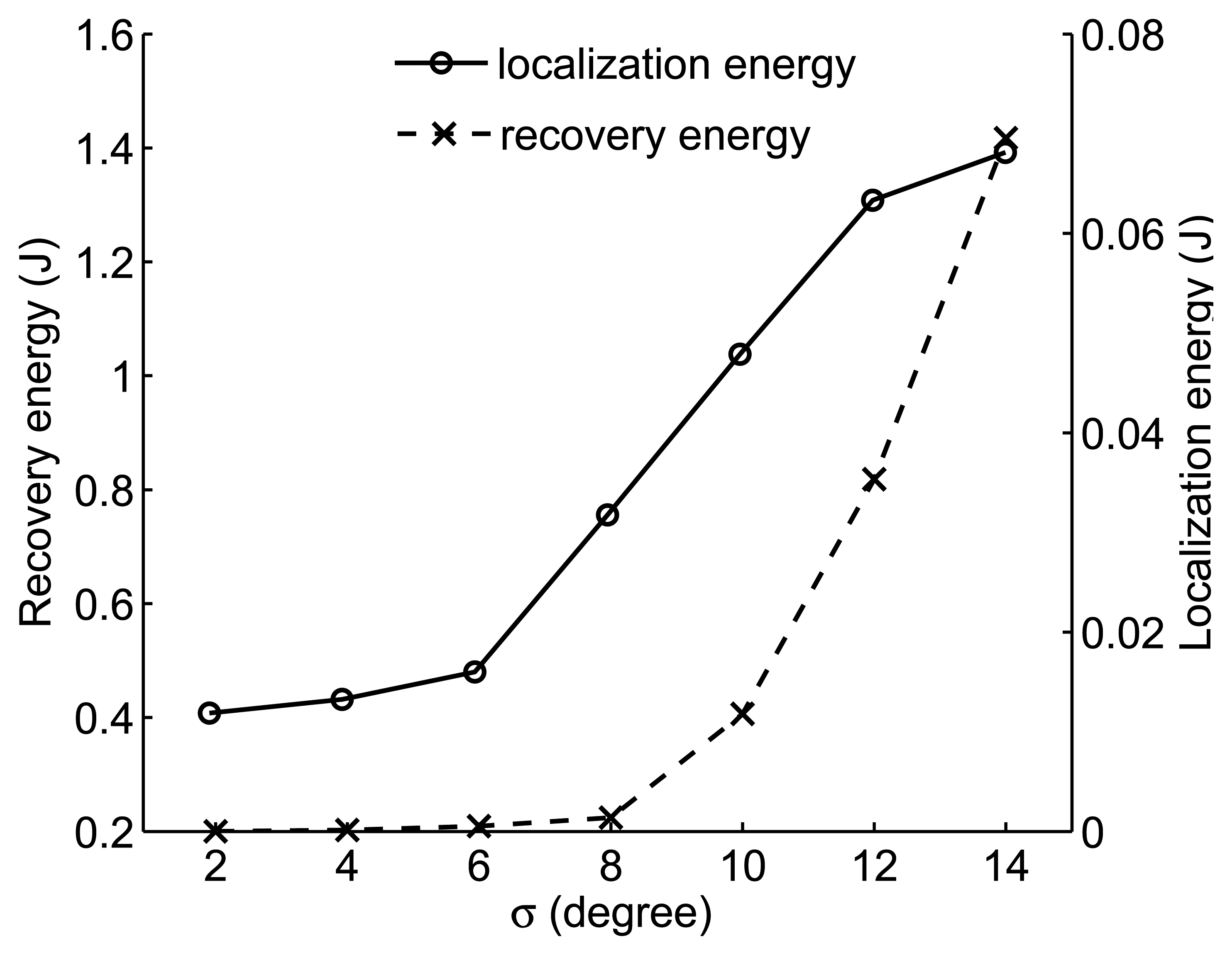
4.4. Impact of sensor node observation deviation
Standard deviation of sensor node observation σ is another crucial factor that impacts the network energy consumption. Moreover, σ is closely relative to the overhead of sensor node. Obviously, small σ value makes sensor nodes expensive. Because of the large number of sensor nodes, WSN is very sensitive to the overheads of sensor node. To prolong the lifetime of the network and reduce network overhead as well, it is important to design the network with appropriate sensor node accuracy.
Figure 13 shows the impact of σ on the network energy consumption, which are the averages of 100 iterations. When the value of σ increases, the network needs more sensor nodes for collaborative sensing so that the localization error could be smaller than εa. It also becomes much more difficult to reach the accuracy within the limited awakening steps. Both two reasons make recovery mechanism performs more frequently, and the energy consumption for localization and recovery rises.
5. Conclusions
Target tracking applications in WSN require high tracking accuracy and low energy consumption. This paper proposes an energy-efficient optimization approach that enables reorganization of WSNs. The basic idea of the approach is to keep sensor nodes sleeping as long as possible. The proposed target tracking approach typically goes through the two phases of prediction and localization. In the prediction phase, the sink node performs a particle filter algorithm to forecast target movement based on past information and awakens a sensor node near the predicted target location. When the prediction is over, the localization phase starts immediately. The current active sensor node calculates mutual information and energy consumption of candidate sensor nodes, and then selects the most energy-efficient sensor node to locate target collaboratively. In cases where the current sensor node is blind to the target, the recovery phase is added after the prediction phase to recapture the target by awakening extra sensor nodes which are selected by a pre-performed genetic algorithm. At last, a series of experiments are carried out to investigate the performance of our approach. The impacts of localization error upper bound and standard sensor node observation deviation are also studied. It is verified that the proposed approach can satisfy tracking accuracy well. Moreover, it can reduce energy consumption, prolong the lifetime of network and decrease network overheads.
Acknowledgments
This paper is sponsored by National Grand Research 973 Program of China (No. 2006CB303000) and National Natural Science Foundation of China (No. 60673176, No.60373014, No. 50175056).
References and Notes
- Wang, X.; Wang, S. Collaborative signal processing for target tracking in distributed wireless sensor networks. Journal of Parallel and Distributed Computing 2007, 67, 501–515. [Google Scholar]
- Zhao, F.; Shin, J.; Reich, J. Information-driven dynamic sensor collaboration for tracking applications. IEEE Signal Processing Magazine 2002, 19, 61–72. [Google Scholar]
- Winter, J.; Xu, Y.; Lee, W. C. Prediction based strategies for energy saving in object tracking sensor networks. IEEE International Conference on Mobile Data Management 2004, 346–357. [Google Scholar]
- Xu, Y.; Lee, W. C. On localized prediction for power efficient object tracking in sensor networks. The Proceedings of Distributed Computing Systems Workshops 2003, 434–439. [Google Scholar]
- Guo, Z.; Zhou, M.; Lev, Z. Optimal tracking interval for predictive tracking in wireless sensor network. IEEE Communications Letters 2005, 7, 438–449. [Google Scholar]
- Yeow, W.; Tham, C.; Wong, W. Energy Efficient Multiple Target Tracking in Wireless Sensor Networks. IEEE Transaction on Vehicular Technology 2007, 56, 918–928. [Google Scholar]
- Pahalawatta, P.; Pappas, T.; Katsaggelos, A. Optimal sensor selection for video-based target tracking in a wireless sensor network. Proceedings of the International Conference on Image Processing; 2004; 5, pp. 3073–3076. [Google Scholar]
- Wang, H.; Yao, K.; Estrin, D. Information-theoretic approaches for sensor selection and placement in sensor networks for target localization and tracking. Journal of Communications and Networks 2004, 36–45. [Google Scholar]
- Kaplan, L. Global node selection for localization in a distributed sensor network. IEEE Transactions on Aerospace and Electronic Systems 2006, 42, 113–135. [Google Scholar]
- Yang, L.; Feng, C.; Rozenblit, J. W. Adaptive tracking in distributed wireless sensor networks. Proceedings of the 13th Annual IEEE International Symposium and Workshop on Engineering of Computer Based Systems; 2006. [Google Scholar]
- Zhong, L. C..; Shah, R.; Guo, C. An ultra-low power and distributed access protocol for broadband wireless sensor networks. IEEE Broadband Wireless Summit 2001. [Google Scholar]
- Jung, E. S.; Vaidya, N. H. A power control MAC protocol for ad hoc networks. ACM Proceedings of the 8th Annual International Conference on Mobile Computing and Networking; 2002; pp. 36–47. [Google Scholar]
- Zou, Y.; Chakrabarty, K. Sensor deployment and target localization based on virtual forces. Proceedings of the IEEE INFOCOM 2003, 1293–1303. [Google Scholar]
- Li, S.; Xu, C.; Pan, W. Sensor deployment optimization for detecting maneuvering targets. Proceedings of the 7th International Conference on Information Fusion; 2005; pp. 1629–1635. [Google Scholar]
- Liu, J.; Koutsoukos, X.; Reich, J. Sensing field: coverage characterization in distributed sensor networks. IEEE International Conference on Acoustics, Speech, and Signal Processing; 2003; pp. 173–176. [Google Scholar]
- Fox, D.; Hightower, J.; Liao, L. Bayesian filtering for location estimation. IEEE Pervasive Computing 2003, 2, 24–33. [Google Scholar]
- Heinzelman, W. R.; Chandrakasan, A.; Balakrishnan, H. Energy-efficient communication protocol for wireless micro sensor networks. International Conference on System Sciences; 2000; pp. 1–10. [Google Scholar]
- Duh, F. B.; Lin, C. T. Tracking a maneuvering target using neural fuzzy network. IEEE Trans. Syst. , Man, and Cybernetics 2004, 34, 16–33. [Google Scholar]
- Merwe, R.; Doucet, A.; Freitas, N.; Wan, E. The unscented particle filter. In Department of Engineering; Cambridge University; Technical Report CUED/F-INFENG/TR 380; 2000. [Google Scholar]
- Gustafsson, F.; Gunnarsson, F.; Bergman, N. Particle filters for positioning, navigation and tracking. IEEE Transaction on Signal Processing 2002, 50, 425–437. [Google Scholar]
- Wang, X.; Wang, S. An improved particle filter for target tracking in sensor system. Sensors 2007, 7, 144–156. [Google Scholar]
- Vaswani, N. Bound on errors in particle filtering with incorrect model assumptions and its implication for change detection. IEEE International Conference on Acoustics, Speech, and Signal Processing; 2004; pp. 17–21. [Google Scholar]
- Ertin, E.; Fisher, J. W.; Lee, C. P. Maximum mutual information principle for dynamic sensor query problems. IPSN2003 2003, 405–416. [Google Scholar]
- Liu, J.; Reich, J.; Zhao, F. Collaborative in-network processing for target tracking. Journal on Applied Signal Processing 2003, 23, 378–391. [Google Scholar]
- Noto, M.; Sato, H. A method for the shortest path search by extended dijkstra algorithm. IEEE International Conference on Systems, Man, and Cybernetics 2000, 3, 2216–2320. [Google Scholar]
- Burne, R. A.; Buczak, A. L.; Jin, Y. C. A self-organizing, cooperative sensor network for remote surveillance: current result. Proceedings of SPIE 13th Annual International Symposium on AeroSense Conference; 1999; pp. 238–248. [Google Scholar]
Figure 1.
Sensor node detection model with different parameters.
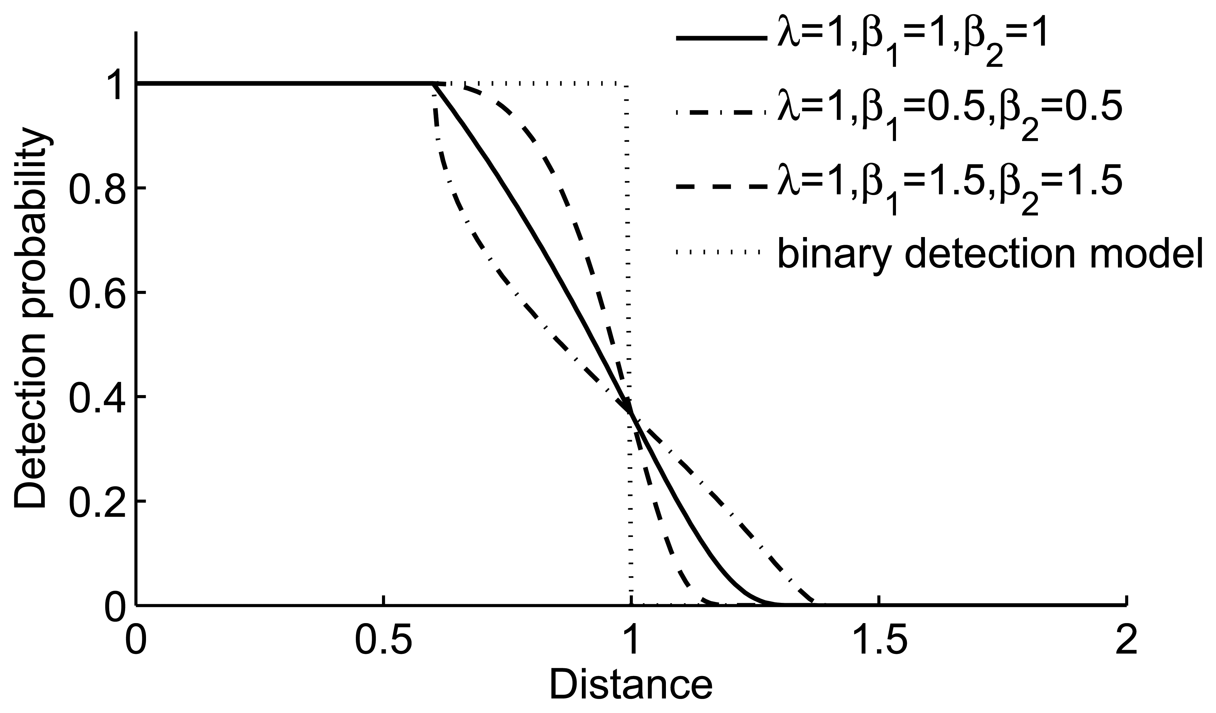
Figure 2.
Collaborative target localization scenario.
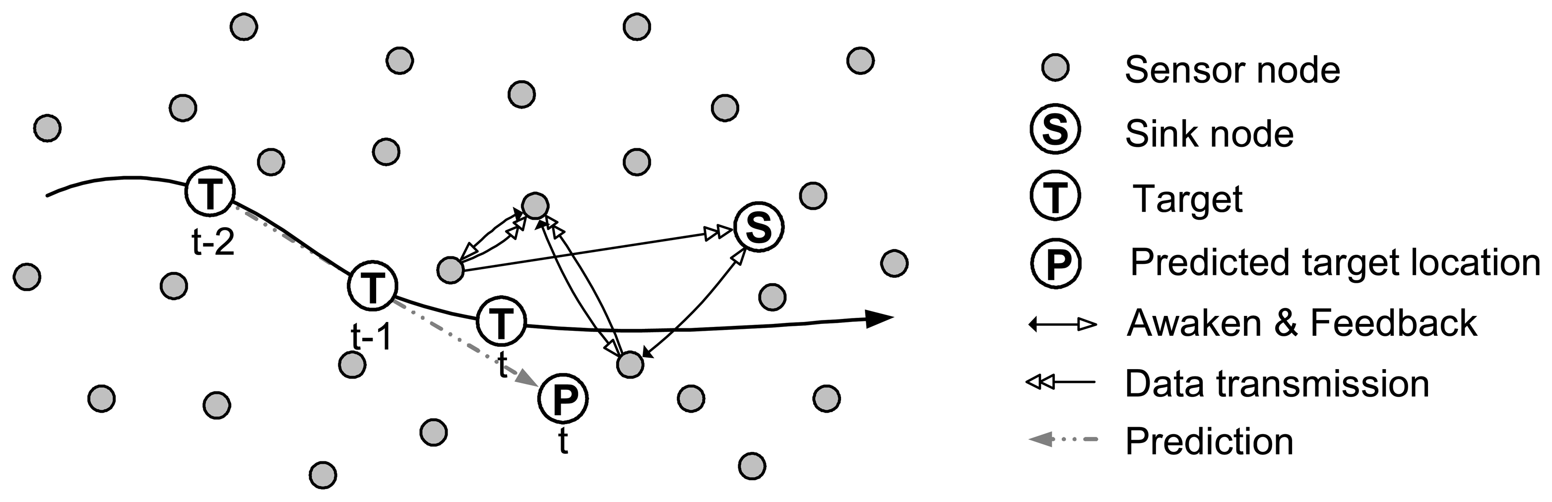
Figure 3.
Packet format for target location distribution.

Figure 4.
Recovery mechanism for target tracking failure.

Figure 5.
Recovery sensor nodes selected by GA.
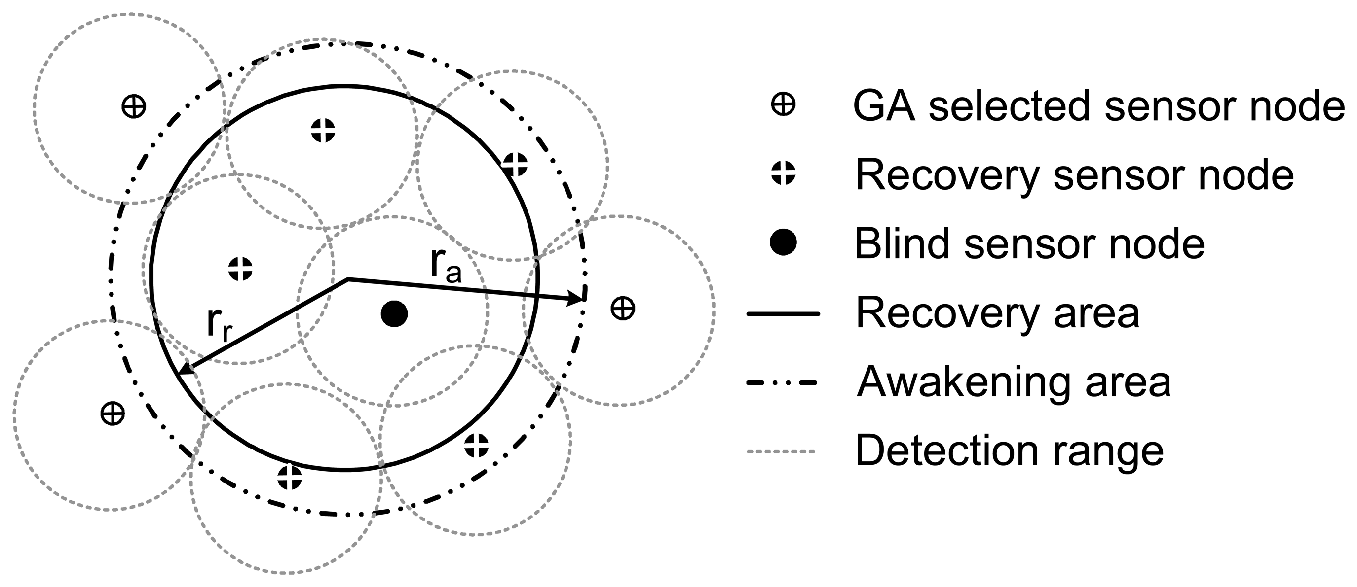
Figure 6.
Sensor node deployment and tracked vehicle trajectory.

Figure 7.
Prediction error and distance between predicted location and the predicted sensor node.

Figure 8.
Recovery mechanism to find the missing target.

Figure 9.
Tracking result with a localization error upper bound of 4 m.
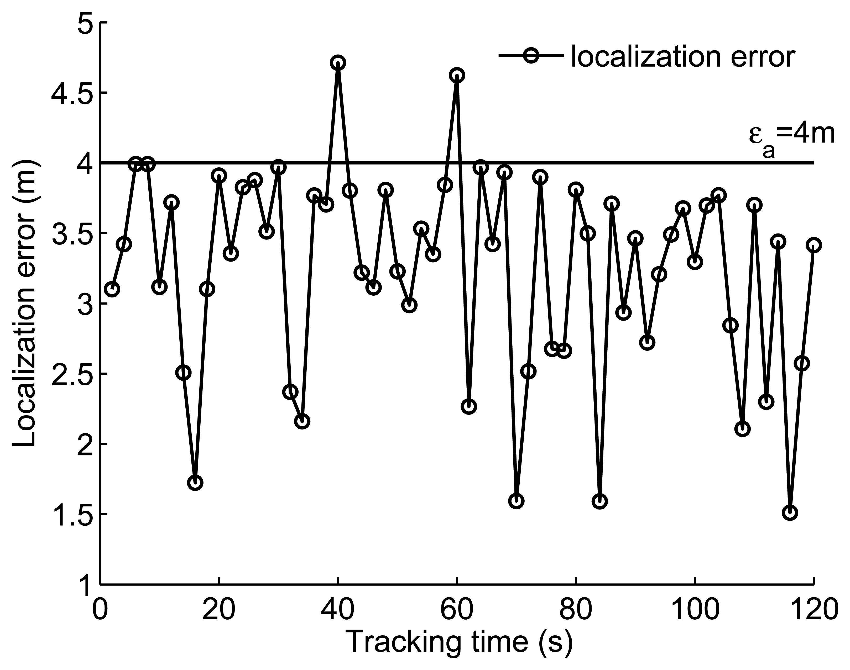
Figure 10.
Energy consumption of WSN in 60 tracking periods.
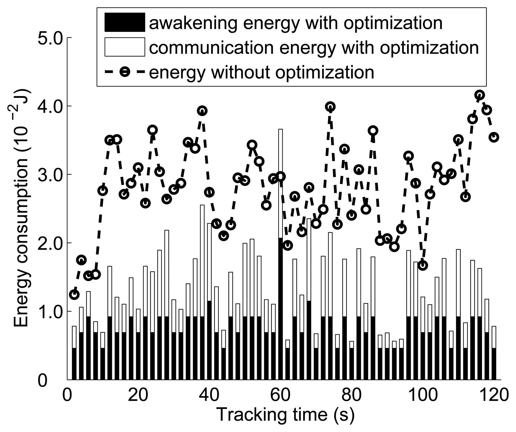
Figure 11.
Impact of localization error upper bound on energy consumption.
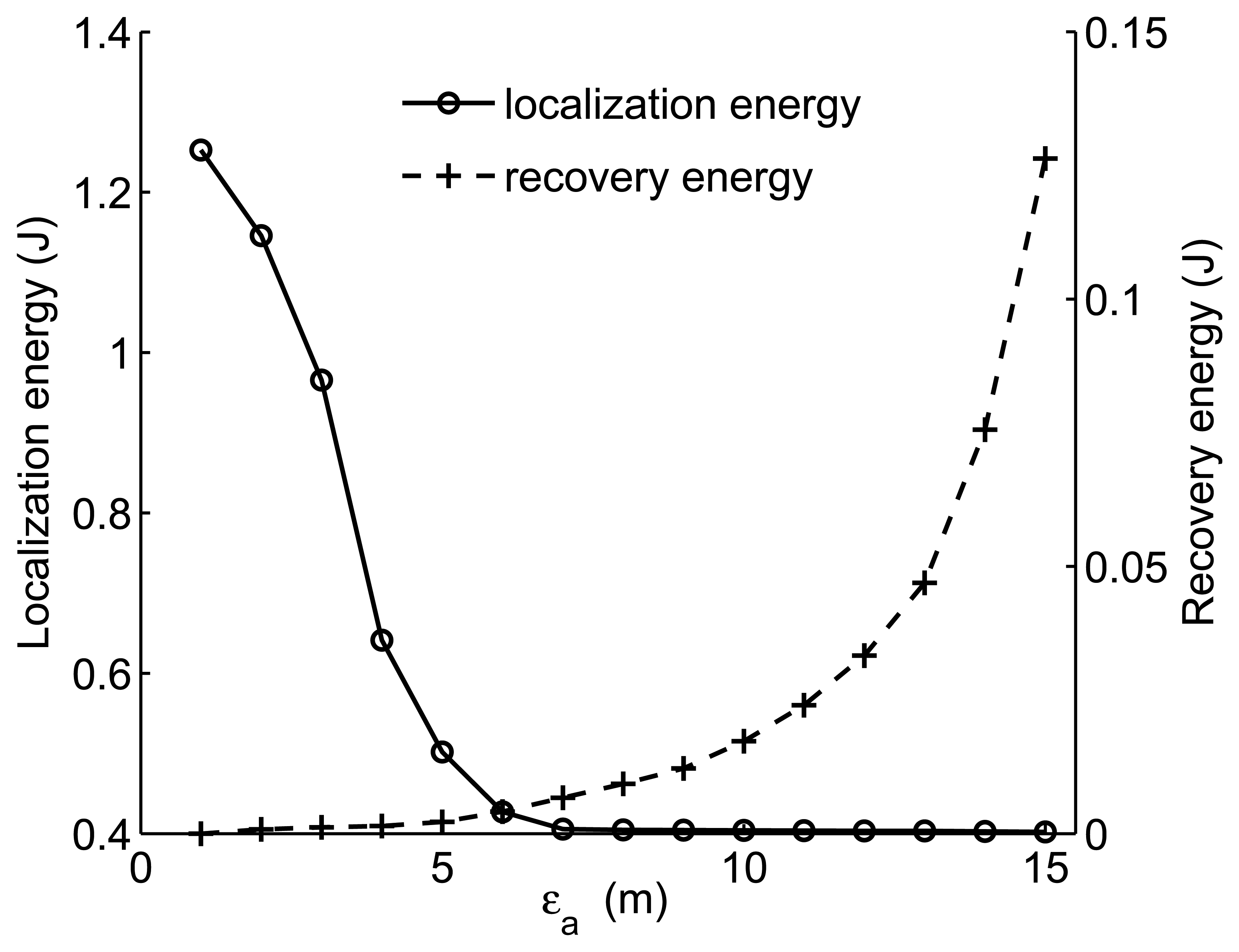
Figure 12.
Total energy consumption of WSN vs. localization error upper bound.
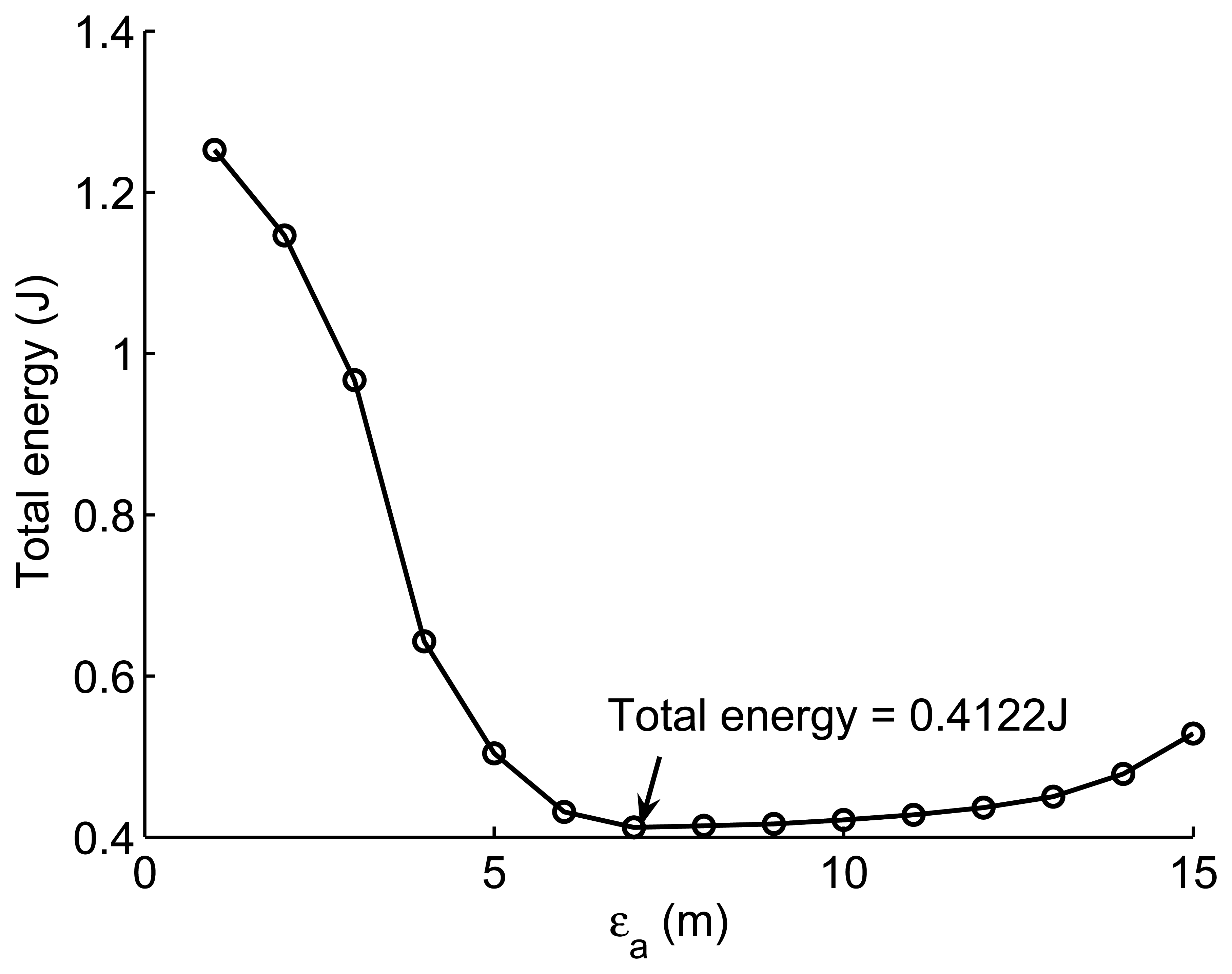
Figure 13.
Impact of sensor node observation standard deviation on energy consumption.

| Component | Mode | Energy consumption (mW) |
|---|---|---|
| Radio | Transmission | 35+PT |
| Radio | Receiving | 35+PR |
| Sensor | Active | 10 |
| MCU | Active | 20 |
| Parameters | Value |
|---|---|
| Transmitter circuitry (Ete) | 50nJ/bit |
| Transmit amplifier (εamp) | 100pJ/bit/m2 |
| Receiver circuitry (Ere) | 50nJ/bit |
© 2007 by MDPI ( http://www.mdpi.org). Reproduction is permitted for noncommercial purposes.
Share and Cite
MDPI and ACS Style
Wang, X.; Ding, L.; Bi, D.-W.; Wang, S. Energy-efficient Optimization of Reorganization-Enabled Wireless Sensor Networks. Sensors 2007, 7, 1793-1816. https://doi.org/10.3390/s7091793
AMA Style
Wang X, Ding L, Bi D-W, Wang S. Energy-efficient Optimization of Reorganization-Enabled Wireless Sensor Networks. Sensors. 2007; 7(9):1793-1816. https://doi.org/10.3390/s7091793
Chicago/Turabian StyleWang, Xue, Liang Ding, Dao-Wei Bi, and Sheng Wang. 2007. "Energy-efficient Optimization of Reorganization-Enabled Wireless Sensor Networks" Sensors 7, no. 9: 1793-1816. https://doi.org/10.3390/s7091793