Models of Hydrogel Swelling with Applications to Hydration Sensing

1
Northern Arizona University, Dept. of Physics, Flagstaff, AZ 86011, USA
2
Cantimer, Inc., Menlo Park, CA 94025, USA
*
Author to whom correspondence should be addressed.
Sensors 2007, 7(9), 1980-1991; https://doi.org/10.3390/s7091980
Submission received: 7 September 2007
/
Accepted: 21 September 2007
/
Published: 25 September 2007
Abstract
:Hydrogels, polymers and various other composite materials may be used in sensing applications in which the swelling or de-swelling of the material in response to some analyte is converted via a transducer to a measurable signal. In this paper, we analyze models used to predict the swelling behavior of hydrogels that may be used in applications related to hydration monitoring in humans. Preliminary experimental data related to osmolality changes in fluids is presented to compare to the theoretical models. Overall, good experimental agreement with the models is achieved.
1. Introduction
The swelling behavior (swelling or de-swelling) of hydrogels (gels) and polymers may be described using many different models. Understanding these models, and the situations in which they may apply, is important with regard to the use of these materials in sensors that make use of the swelling of the material to detect certain analytes. Sensors that currently use these materials as the active sensing element include coated microcantilever sensors [1], embedded piezoresistive microcantilever sensors [2,3], and chemiresistor sensors [4,5]. These sensors may be used in a variety of applications including sensing of volatile organic compounds [5,6], various gases [7,8], biological molecules [9-11], and other analytes.
Equilibrium hydrogel swelling refers to the steady-state, before and after conditions of the gel when a volume change has occurred as a result of exposure to a solvent (analyte). Equilibrium theory is based on a statistical mechanics treatment of the initial and final state of the gel. This type of equilibrium theory has been well described in the literature [12,13], and may be useful in certain situations in which the transient behavior of the gel does not need to be described. In most real-world sensing applications, however, we will need to describe the swelling behavior of the gel material in a more real-time fashion. This will require the use of dynamic hydrogel swelling theory. As with steady-state theory, there is considerable literature published describing the dynamic swelling of various hydrogel materials.
Most dynamic gel swelling models are based in some way on Fick's laws of diffusion. For example, in one dimension, Fick's second law of diffusion (Equation 1) may used to obtain the time-dependent concentration profile of a diffusing species (analyte) in a gel when the concentration of the diffusion species, c, and the diffusion coefficient D are known.
In many cases, Fick's second law is adequate for a description of gel swelling owing to diffusion. For many gels, we must also consider the mass transport of solvent or analyte molecules via convection mechanisms as well. A modified form of Fick's second law, in which there is an additive term to account for convection effects [14], is shown in Equation 2.
In this equation, v represents the “convective velocity” of the glassy/rubbery front of solvent and gel molecules progressing through the gel via convective means. In many systems that do not exhibit much swelling, where the relaxation time of the polymer is much shorter than the characteristic diffusion time for solvent transport, standard Fickian diffusion is generally observed [15]. Here, solvent transport is controlled by a simple concentration gradient, and solvent uptake by the material exhibits 1/√t dependence, with the resulting swelling exhibiting √t dependence (Equation 1). When gel relaxation is the predominant mechanism involved in solvent transport (convection), time-independent diffusion is observed [15], and the swelling would depend linearly with time t. In many cases, however, analyte uptake actually results in an intermediate type of transport mechanism, which is referred to as anomalous transport [16]. In this paper, we will look at numerical and closed-form solutions to anomalous diffusion models, and compare their predictions of gel swelling and de-swelling to preliminary data we have taken on a PVA-based gel system with applications in hydration monitoring.
2. Anomalous Diffusion Models
The solutions to Equation 2 generally fall into three categories: approximate methods, numerical methods, and closed-form solutions. For this paper, dealing with applications in hydration monitoring, we will focus primarily on the numerical and closed-form solutions. Approximate solutions to Equation 2 may also be useful in some cases, so a brief outline of these solutions is given. The final change in volume of a gel, ΔV, is usually approximated by a power law [15], for example:
In Equation 3, n is treated as an adjustable parameter and D(x,t) as a function of position and time within the gel. Note that if D were to be constant and n=1/2, then we have pure Fickian diffusion, and if n=1 we would have pure convection dependent diffusion. Values of n lying between ½ and 1 result in anomalous diffusion. The function D(x,t) will depend on many structural and chemical factors of the gel. Many times, D(x,t) is modeled according to the function [17]
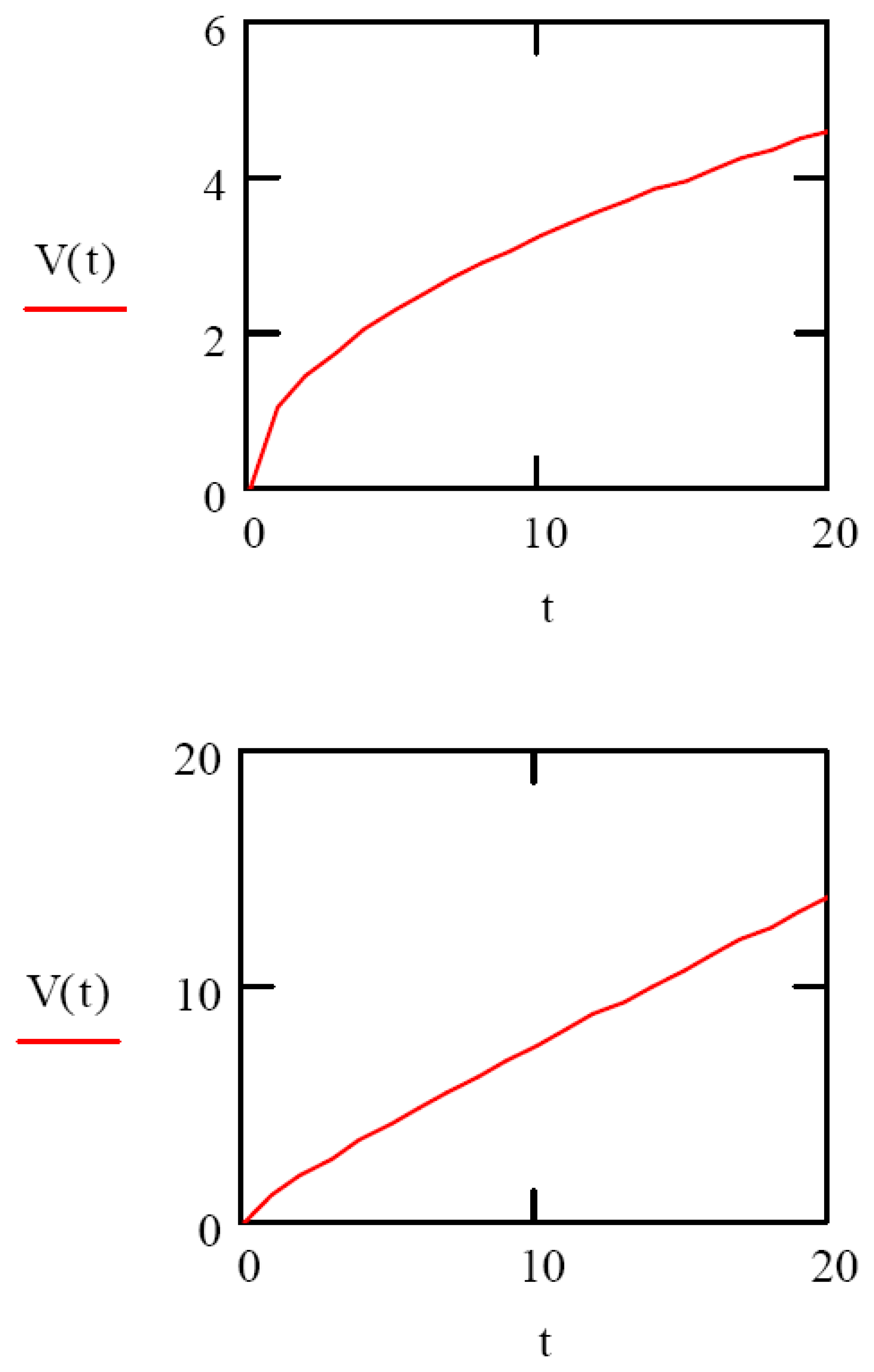
In this expression, ε(x,t) is the volume fraction of solvent in the gel, εr is the gel relaxation constant, and Do is the initial diffusion coefficient. As an illustrative example, we plot two extreme cases of gel volume changes as a function of time using the expression Equation 3 in Figure 1. In Figure 1 (top), using nominal values for D, and n=1/2, we see that the volume change as a function of time is purely Fickian. In Figure 1 (bottom), we use the value n=1 to illustrate the case when the volume change is due to convection only.
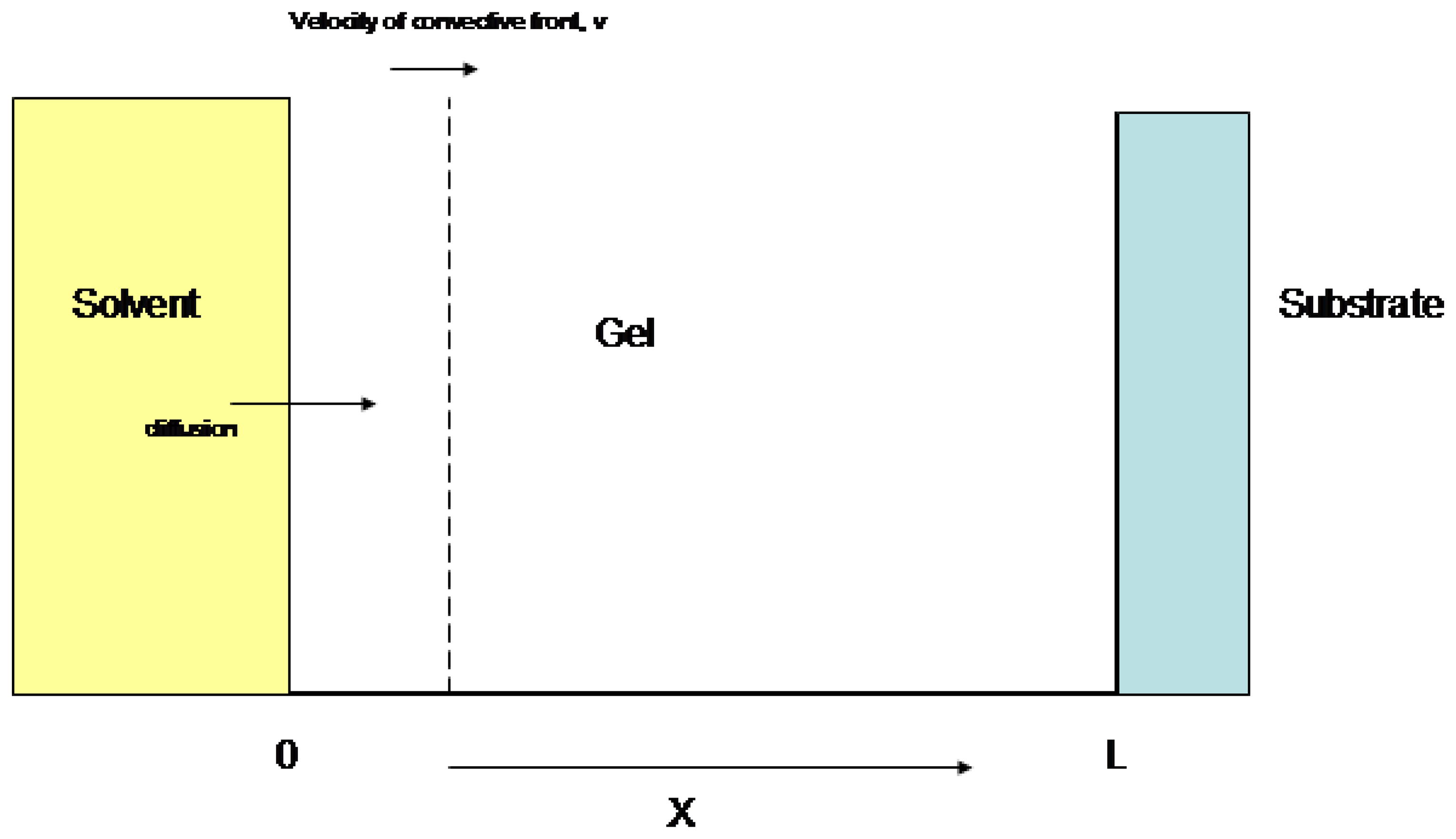
In order to set up the numerical solutions to Equation 2, we need to define many parameters involved in a physical situation similar to that used in embedded piezoresistive microcantilever (EPM) sensors (refer to Figure 2) used in hydration monitoring applications [18]. Typically, these sensors involve a layer of gel (thickness L) deposited on a substrate. In an EPM sensor [2], the microcantilever would be partially embedded in this gel layer in order to measure gel volume changes. Further, let C be the solvent concentration in solution, and D be the Diffusion coefficient of solvent in gel (depends on crosslink density, solvent molecular size, etc.). The value of this parameter describes the relative influence of convection, or gel swelling on the total overall solvent uptake. Finally, let v be the velocity of glassy front (parameter that depends on solvent and gel properties), T be the total diffusion time, f(x) be the initial solvent profile in gel (may be zero if gel starts in dry state), and c(x,t) be the solvent concentration profile in the gel. We will assume that the diffusion into the gel has both a Fickian component and a convective component, taking into account gel relaxation or swelling.
We will also assume some simple boundary conditions for the solution of Equation 2, again referring to Figure 2. We assume:
| c(x,0) = f(x) | initial concentration profile of solvent in gel |
| c(o,t) = C | solvent concentration at solvent-gel interface |
| c(L,t) = 0 | solvent concentration at gel-substrate interface |
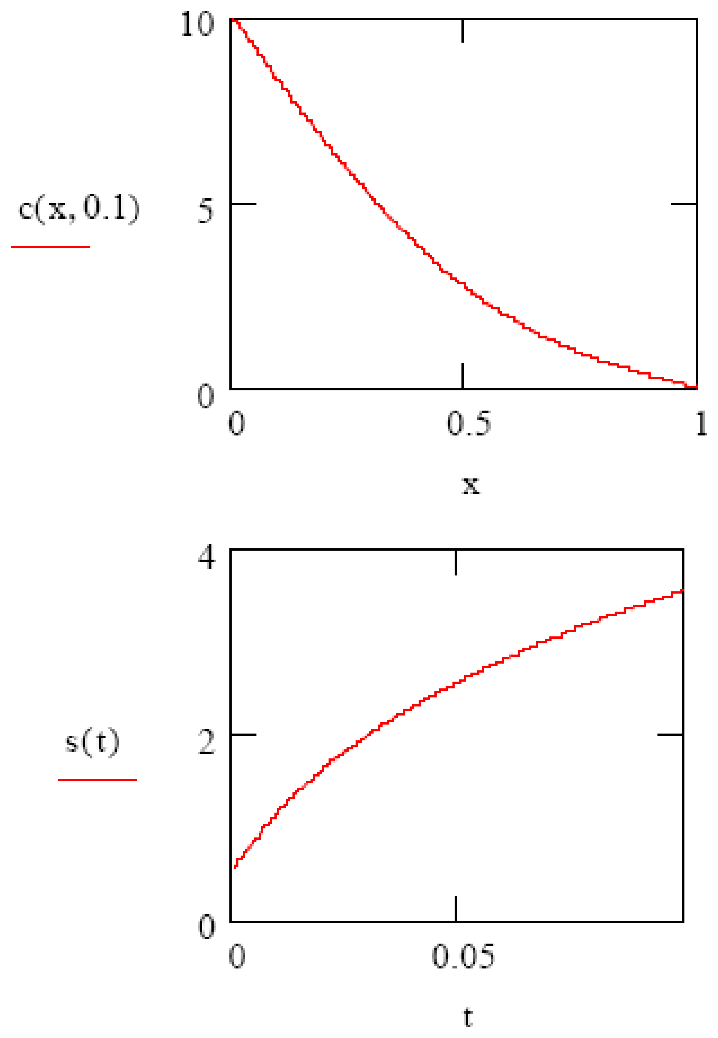
The last boundary condition is needed for the numerical solutions to converge. The solvent concentration at gel-substrate interface will not remain zero forever, however, instead rising as the gel swelling mechanism transitions from the “initial” to the “equilibrium” phases. As an initial calculation, we choose the following arbitrary values: D = 1, L = 1, C= 10, T = 1, v = 0.1, f(x) = 0. In Figure 3, we show the numerical solutions to Equation 2, giving the analyte concentration profile c(x) in the gel at time t=0.1 sec. (top), and the integral of this function s(t), giving the volume change of the gel as a function of time. Note that the appearance of this last plot (Figure 3 bottom) appears in form to be intermediate between the pure Fickian and pure convection gel swelling cases (Figure 1).
The diffusion equation may also be solved in certain circumstances in closed form [19]. Using Fourier transform methods, we may write the solution to Equation 2 in the form
And
These solutions apply to two distinct regions within the gel film. The top equation applies in the region “behind” the convective front, while the second equation, Equation 6, applies to the region in the gel “ahead” of the convective front. We may integrate these two expressions over the appropriate intervals in order to obtain an expression for the total swelling as a function of time
Here, L is the thickness of the gel film. In these expressions D is the Diffusion coefficient, v is the velocity of convective front, t is the time of diffusion experiment, and x = position in gel (x=0 corresponds to gel-solvent interface). We note that since these expressions are valid for the dynamic diffusion region, we must set the total time (t) to some value less than the value of L/v.
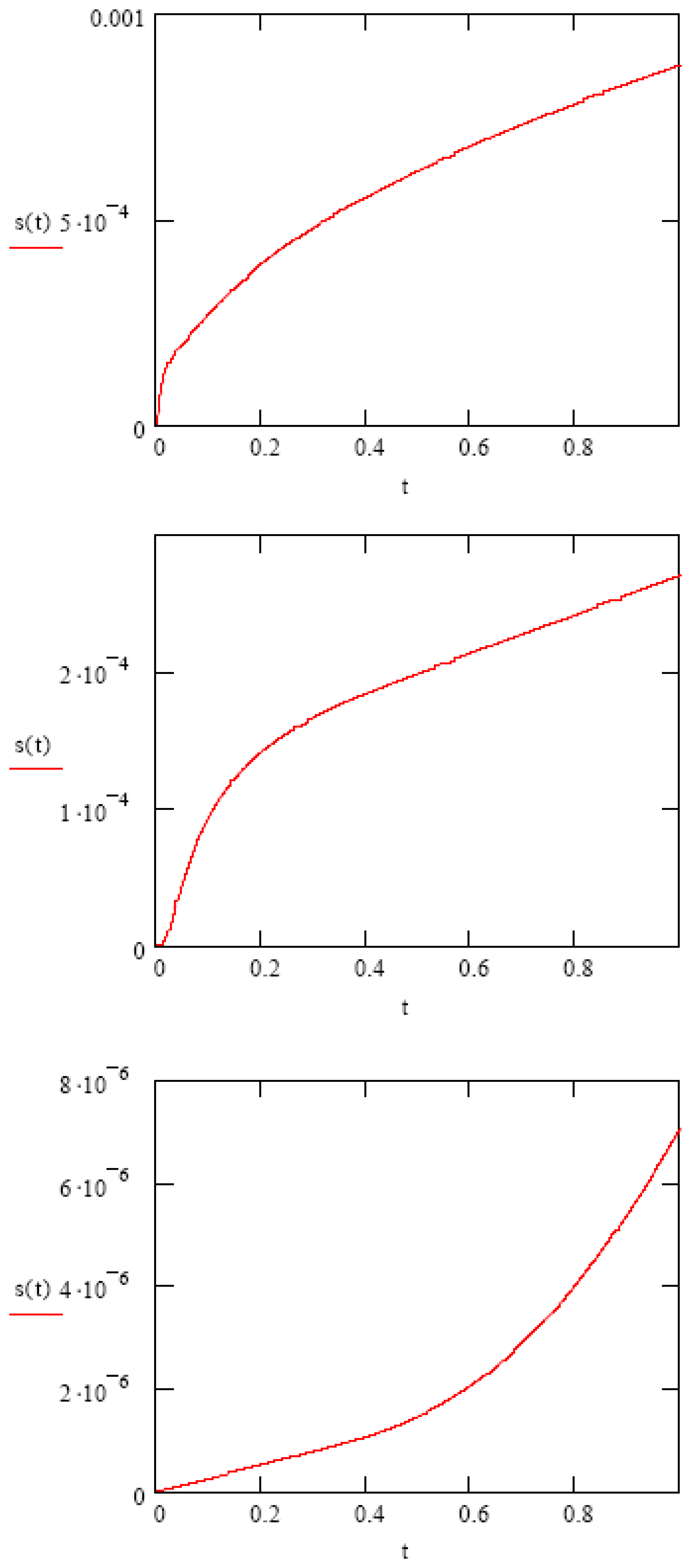
In the next figure (Figure 4), we use published experimentally measured data on crosslink density, diffusion coefficient, and convective front velocity to obtain the swelling profiles of two polymers using equation 7 [15]. In the first example (Figure 4 top), p(HEMA) was prepared with a crosslink density of 0.1 (ratio of crosslinked to non-crosslinked). This is considered to be fairly low crosslinking. The measured diffusion coefficient was 6 × 10⁻⁷ cm2/s, and the experimentally measured front velocity was 3.8 × 10⁻⁶ cm/s. A film thickness of 1 mm is used in the calculation (this is the actual experimental thickness used later), and a diffusion time of 1 second (again, typical for our experiments). This swelling profile is predominantly Fickian, with only a small convective component. In the second example (Figure 4 middle), a moderately crosslinked PVA-c was used. The diffusion coefficient for water in this material is 0.6 × 10⁻⁷ cm2/sec, and the frontal velocity was measured to be 2.4 × 10⁻⁶ cm/s. Again, the gel thickness was 1 mm, and the diffusion time was 1 sec. This swelling profile is anomalous, with both Fickian and convective components. Finally (Figure 4 bottom), a highly crosslinked PVA-c was used. Here, D = 1 × 10⁻⁸ cm2/s, and v = 5 × 10⁻⁶ cm/s. In this case, the diffusion (swelling) profile is predominantly convection, with a small Fickian component.
3. Hydration Monitoring and the Effects of Osmolality
When we look specifically at hydration monitoring [18], it is not just the diffusion or convection of water molecules into the gel that matters, but the effects of the solution osmolality on that diffusion or convection of water molecules into the gel. When we look at the diffusion equation, the only adjustable parameters are the diffusion coefficient D, the convection front velocity v, and the boundary conditions used when the equation is solved. One reasonable assumption may be that the “diffusing species remains water, and water only, even in the more complex solutions used for the hydration monitor application. If this is the case, or nearly the case, then the diffusion coefficient D, and the front velocity v, remain unchanged. Therefore, using this approximation, the only “solvent” under consideration within the gel itself is individual water molecules.
What then, is the effect of osmolality on the swelling? One major component of the solution to Equation 2 is the boundary condition at the solvent-gel interface (x=0 in the examples). Here, we set the value of the solvent concentration in solution, C. If the only solvent under consideration is single water molecules, then there will generally be two factors that change this boundary condition when the osmolality of the solution at the gel surface changes. They are: dissolved proteins and other large molecules – effectively reduce the solvent (water) concentration, and ions in solution when hydrated are no longer “single water molecules”. They become larger structures, in fact, ions surrounded by partially oriented water molecules. If these species are large compared to the open pore sizes in the gel, they will either not diffuse, or will diffuse slowly compared to the single water molecules. The effect of hydrated ions is thus to reduce the solvent concentration at the interface.
Both of these factors will reduce swelling, depending on the relative degree of dissolved proteins and dissolved ions. Also, we would need experimental data to estimate the relative influence of each mechanism. For example, a series of experiments in which only the dissolved proteins, or only the dissolved ions is changed, and the resulting swelling profiles are measured. Once some effective parameters are calculated, then a predictive model may be used determine swelling based on any possible combination of dissolved proteins or ions.
This same procedure, varying only the “solvent concentration” at the solution-gel interface may also be used to predict or model de-swelling. First, the solvent concentration in the gel is at some equilibrium or high value based upon exposure to a “large” solution solvent concentration, C. Then, the solvent concentration is reduced, either through an increase in dissolved ions, or dissolved proteins, or both. Now, the boundary conditions for the solution of Equation 2 become different. The initial solvent profile in the gel, f(x), is not zero, but some large value. The effect of these boundary changes alone is to now allow for diffusion of solvent molecules out of the gel, or de-swelling of the material.
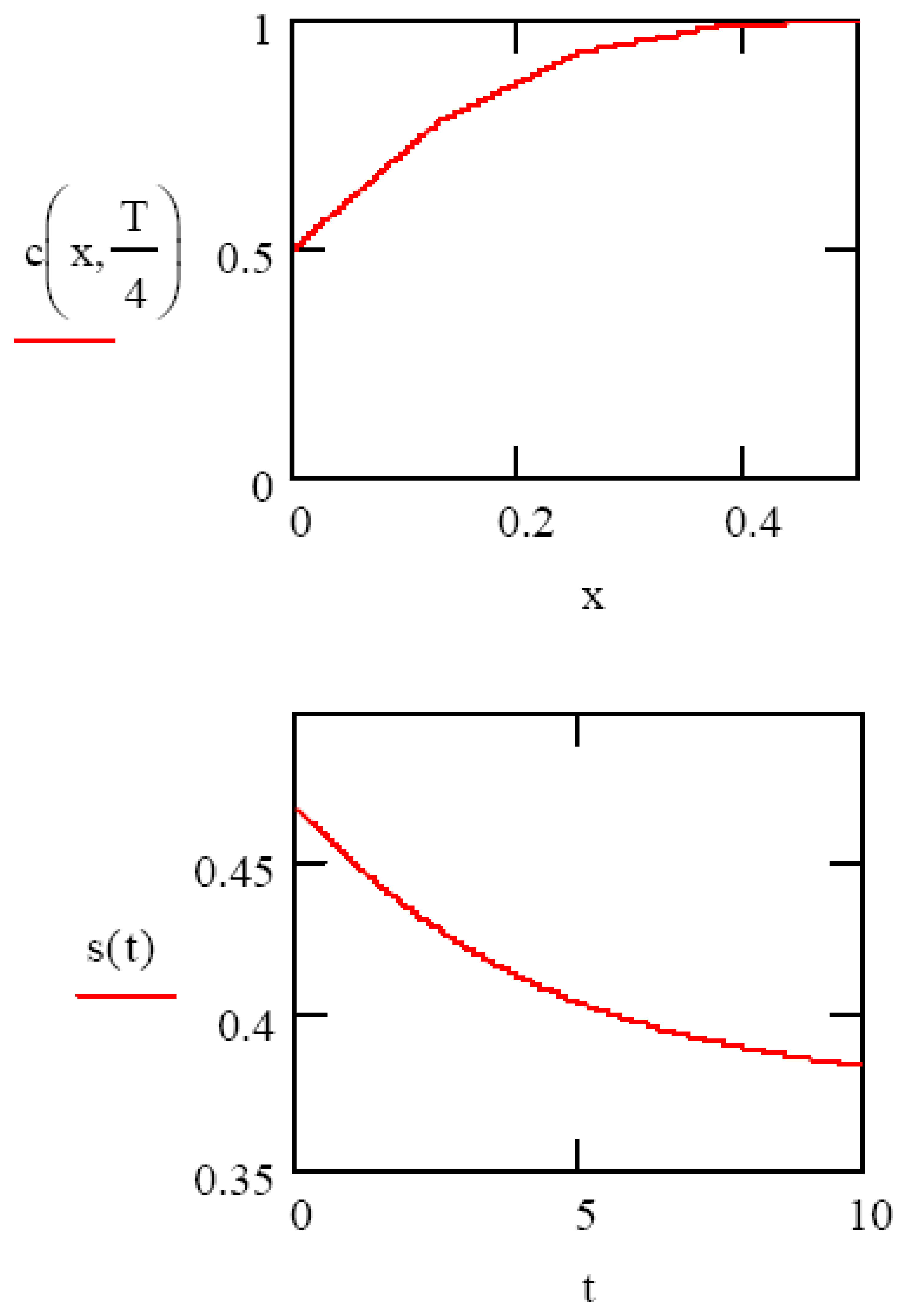
As an example of this, suppose we begin with a gel that has achieved an equilibrium solvent concentration profile of “1” throughout the gel. We then reduce the solvent concentration just outside the gel by some amount, say from 1 to 0.5. The result is the gel will de-swell over time. In this example, the same conditions are used as in the previous “anomalous” diffusion example (Figure 4 middle). Instead of beginning at zero initial solvent concentration in the gel, we use a constant value of 1, an indication that some equilibrium condition has been reached. The solvent concentration outside the gel is then reduced from 1 to 0.5, through an increase in dissolved ions or proteins. Figure 5 shows the numerical solutions in this case, the solvent concentration profile in the gel at time T/4 (top), and the total de-swelling over the full time interval T (bottom).
We can compare these various models to preliminary experimental data taken with an EPM sensor exposed to abrupt changes in solution osmolality and resultant gel de-swelling. An EPM sensor was first fabricated according to previously published techniques [2]. For this experiment the piezoresistive microcantilever was partially embedded in a layer moderately crosslinked PVA, or PVAc synthesized by Cantimer, Inc., Menlo Park, CA. After drying for 72 hours, the sensor was immersed in DI water and allowed to come to full, saturated equilibrium. The microcantilever resistance was then monitored using a simple Wheatstone bridge, and the voltage change across the bridge plotted vs. time. At the time indicated by the arrow in Figure 6, the sensor solution was abruptly changed from DI water to water containing 4% NaCl. This would correspond to a fairly small change in solution osmolality, only a few percent. We can see from Figure 6, the gel begins to de-swell almost immediately. The time dependence of the de-swelling shows a good fit to the theoretically modeled de-swelling shown in Figure 5.
We note that the voltage drop across the cantilever during the osmolality change is approximately 0.3 V. For the current used through the cantilever in these experiments, this corresponds to a cantilever bending of 40 μm. For an initial gel thickness of 1mm, the percentage change in thickness of the gel is approximately 4%. Using the force constant of the cantilever, the contact area of the cantilever on the polymer, and the above deflection, we calculate the additional pressure exerted on the polymer just under the cantilever to be approximately 8 × 10⁴ N/m2, or about 8/10 of 1 ATM. For the moderately crosslinked polymer used in these experiments, we feel that the effects of this additional pressure are very small when compared with the other swelling mechanisms involved. We have also previously studied the swelling/de-swelling reversibility of material as the solution osmolality is changed then brought back to original values [18]. This previous study indicated almost perfect reproducibility during these changes.
4. Conclusions
The swelling behavior of hydrogels has been studied extensively in the literature. Several models and mathematical approaches may be used to describe the swelling or de-swelling of these gels. For the type of gels used in EPM sensors, models of “anomalous” gel swelling most accurately take into account the mechanisms needed to accurately predict the gel swelling behavior. Using anomalous swelling theory, we can use numerical or closed-form solutions to obtain predictions for gel swelling as a function of time. Preliminary data taken with PVAc gel EPM sensors show good agreement with predictions during gel de-swelling in solutions in which there are changes in osmolality.
References and Notes
- Thundat, T.; Chen, G.Y.; Warmack, R.J.; Allison, D.P.; Watcher, E.A. Vapor Detection Using Resonating Microcantilevers. Anal. Chem. 1995, 67, 519–521. [Google Scholar]
- Porter, T.L.; Eastman, M.P.; Macomber, C.; Delinger, W.G.; Zhine, R. An Embedded Polymer Piezoresistive Microcantilever Sensor. Ultramicroscopy 2003, 97, 365–369. [Google Scholar]
- Porter, T.L.; Eastman, M.P.; Pace, D.L.; Bradley, M. Polymer based materials to be used as the active element in microsensors: A scanning Force Microscopy Study. Scanning 2000, 22, 1–5. [Google Scholar]
- Lundberg, B.; Sundqvist, B. Resistivity of a Composite Conducting Polymer as a Function of Temperature, Pressure, and Environment: Applications as a Pressure and Gas Concentration Transducer. J. Appl. Phys. 1986, 60, 1074–1079. [Google Scholar]
- Lonergan, M.C.; Severin, E.J.; Doleman, B.J.; Beaber, S.A.; Grubbs, R.H.; Lewis, N.S. Array-Based Vapor Sensing Using Chemically Sensitive Carbon Black-Polymer Resistors. Chem. Mater. 1996, 8, 2298–2312. [Google Scholar]
- Porter, T.L.; Eastman, M.P.; Pace, D.L.; Bradley, M. Sensor Based on Piezoresistive Microcantilever Technology. Sensors and Actuators A 2001, 88, 47–51. [Google Scholar]
- Kooser, A.; Gunter, R.L.; Delinger, W.G.; Porter, T.L.; Eastman, M.P. Gas Sensing Using Embedded Piezoresistive Microcantilever Sensors. Sensors and Actuators B 2004, 99(2-3), 430–433. [Google Scholar]
- Porter, T.L.; Vail, T.L.; Eastman, M.P.; Stewart, R.; Reed, J.; Venedam, R.; Delinger, W. A Solid-State Sensor Platform for the Detection of Hydrogen Cyanide Gas. Sensors and Actuators B 2007, 123, 313–317. [Google Scholar]
- Porter, T.L.; Delinger, W.; Kooser, A.; Manygoats, K.; Gunter, R. Viral Detection Using an Embedded Piezoresistive Microcantilever Sensor. Sensors and Actuators A 2003, 107(3), 219–224. [Google Scholar]
- Gunter, R.L.; Zhine, R.; Delinger, W.G.; Manygoats, K.; Kooser, A.; Porter, T.L. Investigation of DNA Sensing Using Piezoresistive Microcantilever Probes. IEEE Sensors Journal 2004, 4(4), 430–433. [Google Scholar]
- Kooser, A.; Manygoats, K.; Eastman, M.P.; Porter, T. L. Investigation of the Antigen Antibody Reaction Between Anti-Bovine Serum Albumin and Bovine Serum Albumin Using Piezoresistive Microcantilever Sensors. Biosensors and Bioelectronics 2003, 19, 503–508. [Google Scholar]
- Flory, P.J.; Rehner, J. Statistical Mechanics of Cross-Linked Polymer Networks. J. Phys. Chem 1943, 11, 512–520. [Google Scholar]
- Flory, P.J.; Rehner, J. Statistical Mechanics of Cross-Linked Polymer Networks II. J. Phys. Chem. 1943, 11, 521–526. [Google Scholar]
- Brazel, C.S.; Peppas, N.A. Dimensionless Analysis of Swelling of Hydrophilic Glassy Polymers With Subsequent Drug Release From Relaxing Structures. Biomaterials 1999, 20, 721–732. [Google Scholar]
- Cussler, E.L. Diffusion - Mass Transfer in fluid Systems; Cambridge University Press: Cambridge, United Kingdom, 1997. [Google Scholar]
- Hopfenberg, H.B.; Frisch, H.L. Transport of Organic Macromolecules in Amorphous Polymers. Polymer Letters 1969, 7, 405–409. [Google Scholar]
- Buchhold, R.; Nakladal, A.; Gerlach, G.; Herold, M.; Gauglitz, G.; Sahre, K.; Eichhorn, K.-J. Swelling Behavior of Thin Anisotropic Polymer Layers. Thin Solid Films 1999, 350, 178–185. [Google Scholar]
- Gunter, R.L.; Delinger, W.; Porter, T.L.; Stewart, R.; Reed, J. Hydration Level Monitoring Using Embedded Piezoresistive Microcantilever Sensors. Medical Engineering and Physics 2005, 27, 215–220. [Google Scholar]
- Farlow, S. J. Partial Differential Equations for Scientists and Engineers; Dover; New York, 1993. [Google Scholar]
Figure 1.
(top) Purely Fickian volume change as a function of time (n=1/2), and volume change owing to convection (bottom) only (n=1).
Figure 1.
(top) Purely Fickian volume change as a function of time (n=1/2), and volume change owing to convection (bottom) only (n=1).

Figure 2.
Schematic setup of EPM sensor with sensing gel layer on fixed substrate.

Figure 3.
(top) Numerical solution to Equation 2 showing analyte (or solvent) concentration in gel at time t=0.1 sec. (bottom) Resultant gel swelling as a function of time.
Figure 3.
(top) Numerical solution to Equation 2 showing analyte (or solvent) concentration in gel at time t=0.1 sec. (bottom) Resultant gel swelling as a function of time.

Figure 4.
Closed form models of Fickian (top), anomalous (middle), and convective (bottom) diffusion into a gel and the resultant gel swelling.
Figure 4.
Closed form models of Fickian (top), anomalous (middle), and convective (bottom) diffusion into a gel and the resultant gel swelling.

Figure 5.
Solvent concentration (top) and volume change (bottom) as a result of gel de-swelling. Osmolality outside of gel has risen to a higher value after gel reached equilibrium with a lower osmolality solution.
Figure 5.
Solvent concentration (top) and volume change (bottom) as a result of gel de-swelling. Osmolality outside of gel has risen to a higher value after gel reached equilibrium with a lower osmolality solution.

Figure 6.
Experimental PVAc gel de-swelling swing to osmolality change. The sensor was moved abruptly from DI water to 4% NaCl solution at the time indicated by the arrow.
Figure 6.
Experimental PVAc gel de-swelling swing to osmolality change. The sensor was moved abruptly from DI water to 4% NaCl solution at the time indicated by the arrow.

© 2007 by MDPI ( http://www.mdpi.org). Reproduction is permitted for noncommercial purposes.
Share and Cite
MDPI and ACS Style
Porter, T.L.; Stewart, R.; Reed, J.; Morton, K. Models of Hydrogel Swelling with Applications to Hydration Sensing. Sensors 2007, 7, 1980-1991. https://doi.org/10.3390/s7091980
AMA Style
Porter TL, Stewart R, Reed J, Morton K. Models of Hydrogel Swelling with Applications to Hydration Sensing. Sensors. 2007; 7(9):1980-1991. https://doi.org/10.3390/s7091980
Chicago/Turabian StylePorter, Timothy L., Ray Stewart, Jim Reed, and Kathryn Morton. 2007. "Models of Hydrogel Swelling with Applications to Hydration Sensing" Sensors 7, no. 9: 1980-1991. https://doi.org/10.3390/s7091980