Application of Multiplexed FBG and PZT Impedance Sensors for Health Monitoring of Rocks

1
School of Civil and Environmental Engineering, Nanyang Technological University, 50 Nanyang Avenue, Singapore 639798
2
Building and Infrastructure Division, Defense Science & Technology Agency, Singapore 109679
*
Author to whom correspondence should be addressed.
Sensors 2008, 8(1), 271-289; https://doi.org/10.3390/s8010271
Submission received: 23 December 2007
/
Accepted: 11 January 2008
/
Published: 21 January 2008
(This article belongs to the Special Issue Sensors for Urban Environmental Monitoring)
Abstract
:Reliable structural health monitoring (SHM) including nondestructive evaluation (NDE) is essential for safe operation of infrastructure systems. Effective monitoring of the rock components of civil infrastructures such as tunnels and caverns remains challenging. The feasibility of employing smart optical fibre sensor (OFS) and piezoelectric impedance sensor made up of lead zirconate titanate (PZT) for comprehensive health monitoring of rocks, covering load history monitoring/retrieval as well as damage assessment is presented in this paper. The rock specimens are subjected to cyclic loading and their conditions are continuously monitored using OFS and PZT sensors. OFS based multiplexed fibre Bragg grating (FBG) sensors are surface bonded on the rock specimens. Their strain sensing performance is compared with the conventional electric strain gauges (ESGs). In addition, PZT patches are also bonded on the specimens to study the damage pattern during different loading cycles. Unlike the FBGs or ESGs, PZT patches are used as bi-functional sensors and actuators, enabling them to be efficient detectors of incipient damages using the principle of electromechanical impedance. The experimental study demonstrated superior performance of these smart FBG and PZT impedance sensors. This work is expected to be useful for SHM based NDE application of rock structures such as caverns and tunnels.
1. Introduction
Owing to the scarcity of land, Singapore is looking towards underground space (i.e., tunnels and caverns) to meet the ever increasing residential, commercial and transportation demands. However, constructing underground structures is not an easy task, especially in the densely populated areas like the central business district. Lack of comprehensive monitoring can seriously endanger the lives of the construction personnel as well as the safety of the employees/ residents in the buildings or the motorists traveling nearby. This is proven by the tunnel collapse at the Heathrow Airport in London (during October 1994) and that of the Nicoll Highway in Singapore (during April 2004). There is an increasing demand for providing online structural health monitoring (SHM) systems to underground construction in order to guarantee safety and to optimize financial and natural resources. Civil engineering structures especially underground constructions deteriorate with time as a result of aging of materials, excessive use, overloading, climatic conditions, inadequate maintenance and deficiencies in inspection methods. All these factors contribute to the obsolescence of constructed systems. As a result, timely SHM, retrofit, rehabilitation and replacement become necessary to ensure the safety of the public.
An effective and reliable monitoring system should be supported by high performance sensory technology which fulfill ‘A-to-E’ characteristics as follows, (A)ccuracy: sensor should have a reliable accuracy; (B)enefit: commercial price of the sensor should be in a reasonable cost; (C)ompact: sensor should be small in size, especially for embedded installation inside concrete structure; (D)urable: serviceability of the sensor should be long-lived; and (E)asy: sensor should be easy to operate and time consumed for retrieving data should be close to real time measurement [1]. Bhalla et al. [2] presented a detailed review of the available sensor technologies and methods for comprehensive monitoring with special emphasis on conditions encountered underground. Practical benefits arising out of such monitoring are also highlighted, with the help of several real-life case studies involving underground structures.
Continuous measurement of strains represents an important part of SHM systems. If the locations and orientations of the sensors are selected according to the specific characteristics of the structural system, the measured strains provide valuable information about the integrity, the stiffness and the load level. Existing monitoring systems are primarily based on the conventional sensors such as electric strain gauges (ESGs) operating on electrical or vibrating wire principles. These sensors typically require long cables, are prone to noise and electro-magnetic interference, and are not robust enough to sustain the harsh working conditions encountered underground. Fibre Bragg grating (FBG) sensors which belong to optical fibre sensors (OFS) are promising for monitoring of underground or other civil engineering structures.
Generally damages change the load carrying capacity of structures and results in modified strains. However the strain variations due to the incipient damage are difficult to determine. On the other hand, piezoceramics such as lead zirconate titanate (PZT) based electromechanical impedance (EMI) technique is very promising for detecting the incipient damage [3,4]. Thus, the combination of FBG and PZT technologies result in the essential warning for the possibility of any incipient damage.
Thus, this paper examines a low-cost, reliable and generic SHM and safety monitoring system for continuous real-time monitoring of laboratory sized rock components by using smart multiplexed FBG sensors and PZT impedance sensors. Smart sensing technologies are relatively new, careful laboratory evaluation is essential before they could be employed in real-life monitoring of rock structures such as caverns and tunnels. Another purpose served by laboratory tests is to calibrate PZT sensors against damage for the rocks (granite) encountered in Singapore. Finally, the combination of PZT and FBG for successful SHM is presented.
2. FBG Sensors
Although the formation of fiber gratings was reported in 1978 [5], intensive study on fiber gratings began after a controllable and effective method for their fabrication was devised in 1989 [6]. In recent years, there have been a number of research initiatives towards the development and deployment of FBG based sensors for sensing applications in civil and structural engineering [7-9]. FBG sensors offer a wide number of advantages over traditional sensors. These include immunity to electromagnetic interference, electrically passive, long term stability, light weight, small size, multiplex capabilities, ease of installation and durability. A Bragg grating is a periodic structure, fabricated by exposing a photosensitised fibre to an ultraviolet light. When light from a broad band source interacts with the grating, a single wavelength, known as the Bragg wavelength, is reflected back whereas the rest of the signal is transmitted. An external mechanical strain in the fibre (a stimulus) shifts the Bragg wavelength (response of the fibre) through expansion/contraction of the grating periodicity and the photo elastic effect. Similarly, a temperature variation (stimulus) causes thermal expansion/contraction of the grating periodicity and also changes the refractive index (responses). These effects provide the means of employing the FBG written fibres as the sensor elements for measuring strains and temperatures.
Figure 1 illustrates the working principle of the FBG based strain gauge. When light from a broad band source interacts with the grating, the Bragg wavelength is reflected back whereas the rest of the signal is transmitted. The Bragg wavelength λB depends both on the physical characteristics of the fiber and on the geometrical characteristics of the grating, that is
where neff is the effective refractive index of the mode propagating along the fiber and Λ is the period of the FBG. Both the effective refractive index and the grating period vary with changes in strain Δε, a temperature change ΔT and a pressure change ΔP, imposed on the fiber. An applied strain and pressure will shift the Bragg wavelength through expansion or contraction of the grating periodicity and through the photo elastic effect. Temperature affects the Bragg wavelength through thermal expansion and contraction of the grating periodicity and through thermal dependence of the refractive index. If only the dominant linear effects of these three factors on an FBG sensor are considered, neglecting higher-order cross-sensitivities, then the amount of Bragg wavelength shift is given by [10]
where Kε, KP and KT are the respective wavelength sensitivity coefficients for strain, temperature and pressure for an FBG given by
where ρ11 and ρ12 are the components of the fiber optic strain tensor; v is the Poisson's ratio; ξ is the thermo-optic coefficient; and E is the Young's modulus.
Owing to the harsh environments found in the construction and operation of the underground structures, the sensors selected should be robust, rugged and easy to use and economical. Thus, FBG sensors were selected as one of the smart sensors in this paper, the feasibility and effectiveness of these FBG sensors for monitoring the rock cube are demonstrated in the later experimental sections.
3. Damage Detection Using PZT Impedance Sensors
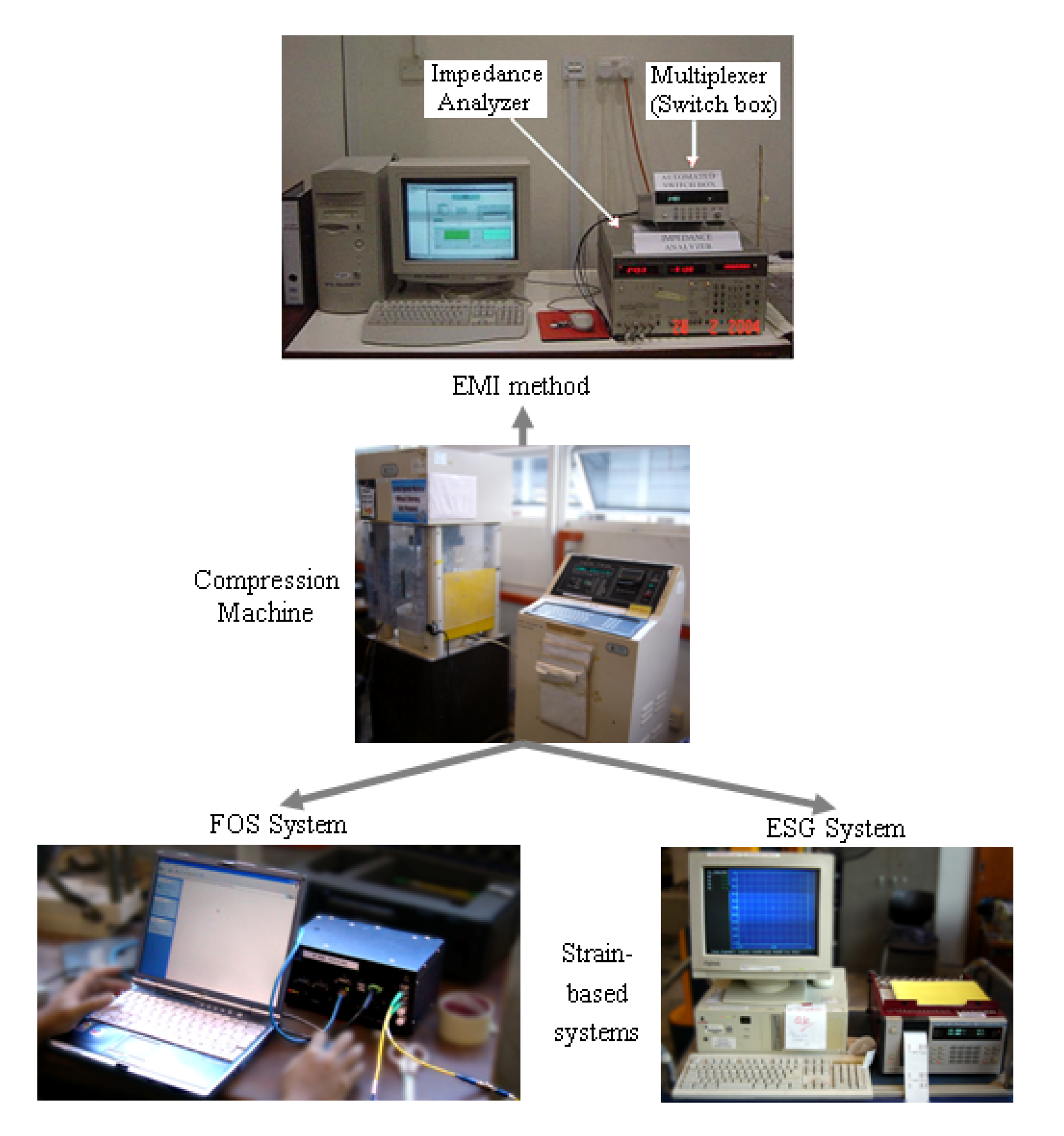
PZT impedance sensors, usually in the shape of small patches, which do not measure direct physical parameters like stress, strain or temperature, are relatively new sensors, barely two decades old. PZT patches are usually bonded on the surface or embedded inside the host structure to be monitored. The basic concept of the electromechanical (EM) impedance (EMI) based SHM approach is that the presence of damage in the host structure will affect its mechanical impedance, and thus the EM admittance (inverse of impedance) of the PZT patch, which can be directly measured by an electrical impedance analyzer, such as the HP 4192A impedance analyzer as shown in Figure 2. The impedance analyzer imposes an alternative voltage signal of 1 volt via a 40-channel multiplex to the bonded PZT patch over the user specified frequency range. The changes in extracted admittance signature are indication of the presence of structural damages, which can be used for damage assessment. The PZT admittance signature is a function of the stiffness, mass and damping of the host structure, and the properties of the PZT patch [11,12]. In principle, the EMI technique is similar to the conventional global vibration techniques. The major difference is only with respect to the frequency range employed, which is typically 30-400 kHz for the EMI techniques against less than 100 Hz for the global vibration technique. The EMI technique has several advantages over the conventional load/stress/strain measurement based techniques, since it does not warrant any complex analytical/numerical modelling of the monitored structure. It employs low-cost and low-power demanding PZT impedance sensors, which can be non-intrusively bonded to the structure and can be interrogated without removal of finishes. Neither complex data processing nor expensive hardware is necessary, and it also does not necessitate the structure to be placed out of service. By means of an array of such patches, damage location and/or severity can be identified [4]. The technique has far greater sensitivity to structural damages than the conventional global vibration techniques. The data acquisition is also much more simplified than the traditional accelerometer-shaker combination employed in the global vibration techniques.
Liang et al. [13] first proposed a one-dimensional impedance approach to model PZT-structure EM interaction. Subsequently, a number of two-dimensional models have been developed [12,14]. For simplicity, Liang's model will be used in this paper. In this model, the host structure is simplified as a skeletal structure and the PZT impedance sensor as a thin bar undergoing axial vibration. Based on the piezoelectric effect of imparting mechanical strain when subjected to an electric field and the converse piezoelectric effect of generating electric charges in response to a mechanical strain, the EM admittance of the PZT sensor is expressed as
where Za and Z are the mechanical impedances of the PZT and the host structure, respectively; j is the imaginary unit; ω is the angular frequency of the driving voltage; wa, la and ha are the width, length and thickness of the PZT patch, respectively;
is the complex Young's modulus of the PZT material at zero electric field; d31 is the piezoelectric constant;
is the complex dielectric constant; η and δ denote the mechanical loss factor and the dielectric loss factor of the PZT material, respectively; κ is the wave number which is related to the angular frequency of excitation ω by
; and ρ is the material density of the structure.
Equation (3) indicates that the EM admittance of PZT sensor is directly related to the mechanical impedance of the host structure. Therefore, any change in the EM admittance signatures is the indication of a change in the structural integrity which may be caused by the appearance of structural damage.
During the last decade, the EMI technique has demonstrated its potential to be an efficient and cost-effective SHM technique for a wide variety of engineering structures. Various issues such as EMI modeling [12,14,15,16], PZT sensing region [17,18], and applications [3,11,19,20,21] related to the EMI technique have been extensively studied.
In all the EMI models, conductance (real part of admittance) is considered to be more important as compared to its counterpart susceptance (imaginary part of admittance) [4,11] and hence it has been used for damage assessment in almost all the applications. This paper demonstrates the feasibility of employing PZT patches for SHM of rocks by means of a detailed experimental study as described in the next section.
4. Health Monitoring of Rocks Using FBG and PZT Sensors
The overall experimental setup is shown in Figure 2, which consists of a compression machine and the EMI, OFS and ESG measurement systems. The EMI system is impedance-based, while the OFS and ESG systems are strain-based. The OFS system consists of an optical spectrum analyzer SM125-500 model [22] which is controlled by a personnel computer (PC). A multiplexed optic fibre is connected to the analyzer and the strain measurements are thus obtained. Another strain measuring system which is based on the ESG sensor is logged by a portable data logger model TDS-302 [23] controlled by a PC to obtain the strain reading at certain predetermined loadings. Lastly, the compression testing and load readout is obtained via a DMG Compression Testing Machine.
A total of three rock specimens (1, 2 and 3) were cut to obtain 150mm cubes from the blast fragments (mostly granite) from a underground construction site in Singapore. All three specimens were instrumented with ESG, PZT and FBG sensors on four side surfaces, leaving the top and bottom surfacees for compression purpose as shown in Figure 3.
First, a single fibre with a total of 5 multiplexed FBG sensors, one of which was the temperature sensor and the other four were strain sensors, was installed on each specimen. The four FBG strain sensors were bonded to the four side surfaces named Face 1, 2, 3 and 4, with one sensor on each face. The temperature sensor is for the temperature compensation purpose, thus it was left free without being bonded to the specimen. Second, one ESG sensor was bonded to each face at the symmetric location of the FBG sensor. Installed in this way, the ESG add FBG sensors were expected to obtain the same strain measument for performance comparison. A total of four ESGs were used for each specimen and they were connected to the data logger with their supplied test leads. Finally, one PZT patch was also installed on each face. All four PZT patches were connected to the impedance analyzer using four pairs of wires. Figure 4 shows the schematic layout of the three types of sensors on one face of a specimen. The PZT patches (grade PIC 151) [24] employed in this study were 15mm square in size and 0.3mm in thickness. The multiplexed FBG strain sensors (model SIFU-SS-CF) [25] and ESG sensors [23] had the same gauge length of 60mm. A two part epoxy adhesive (type RS 850-940) [26] was used in bonding the ESG and PZT patches to the rock cube while the FBG strain sensors were bonded with the Araldite Rapid Fast-setting two part epoxy [27].
The specimens were tested through various load cycles with the DMG compression machine set to a constant loading rate of 330 kN/minute. Readings from the FBG and ESG were taken at predetermined load intervals. The PZT patches were interrogated at a frequency range of 40 to 100 kHz at steps of 0.2 kHz. The admittance signatures were acquired only after each loading cycle was completed and the specimen was fully unloaded. The details of load cycles and the measurement intervals are listed in Table 1.
4.1 Strain measurement using FBG and ESG sensors
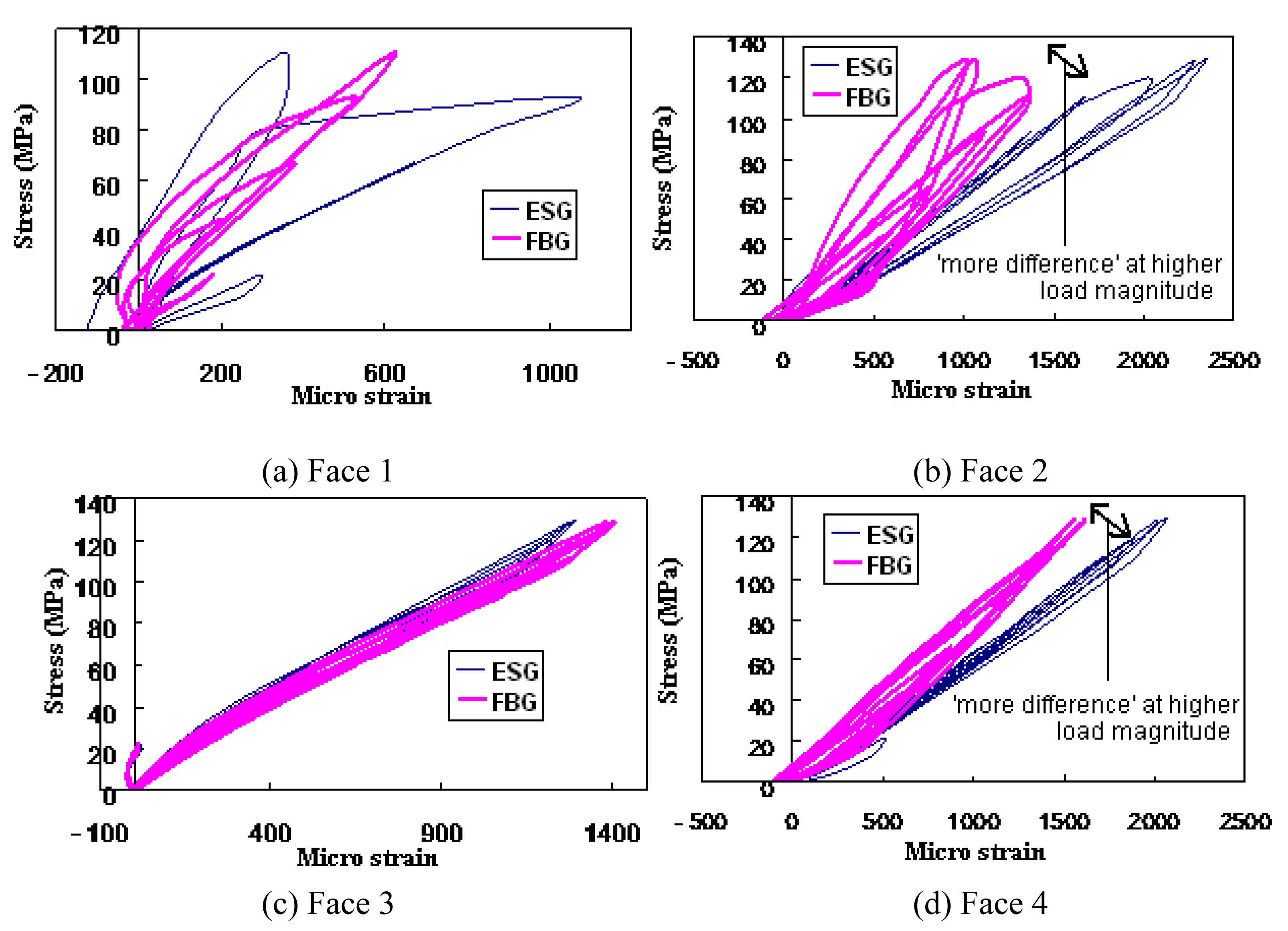
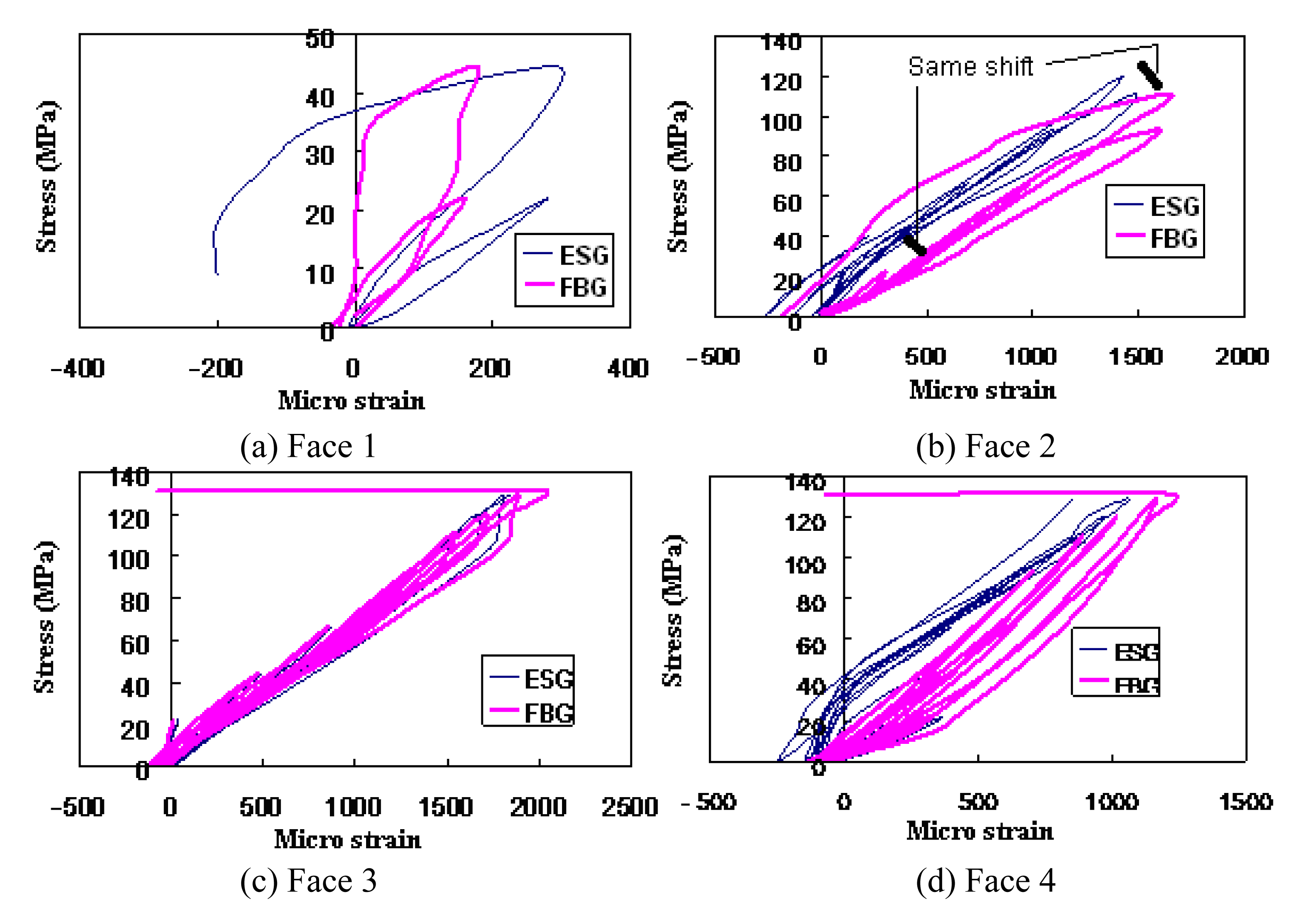
Figures 5, 6 and 7 show the comparison of the stress-strain history of four faces of Specimens 1, 2 and 3 obtained by the ESG and FBG sensors, respectively. However in Figure 6, the strain readings exhibit some abnormality after a few load cycles. The stress-strain curves from the FBG and ESG sensors for Face 1 of Specimen 2 started to show increasing hysteresis and slope after load cycle 1, thus indicating that the area close to the sensors may have developed some damage. Hence, close attention was paid to the surface of this particular face during the test but no obvious cracks were observed. However, during load cycle 6, a loud noise was heard followed by the shearing off of Face 1. The damage was captured and can be seen in Figure 8. Since the fault lies on a plane parallel to the plane of the strain measurement, the stress-strain behaviour was not suitable for the indication of such a potential damage.
In addition, some slight changes in strain history for Faces 2 and 4 of Specimen 3 were observed, i.e., FBG had resulted higher strain variations as compared to ESG (Figure 7). This is because, even though both type of sensors were placed at approximately symmetric locations (Figure 4) the pressure of loading might be a little eccentric (not exactly at the centre) on the specimen. Hence a downward shift of the FBG curves was noticed as compared to the ESG curves for Faces 2 and 4. Nonetheless, the stress-strain curves for all specimens obtained from FBG and ESG sensors match well, i.e., the strain history retrieved by the ESG sensors is similar to that by the FBG strain sensors, which demonstrates the effectiveness of FBG sensors for strain measurement of rocks.
4.2 Admittance signature measured from PZT patches
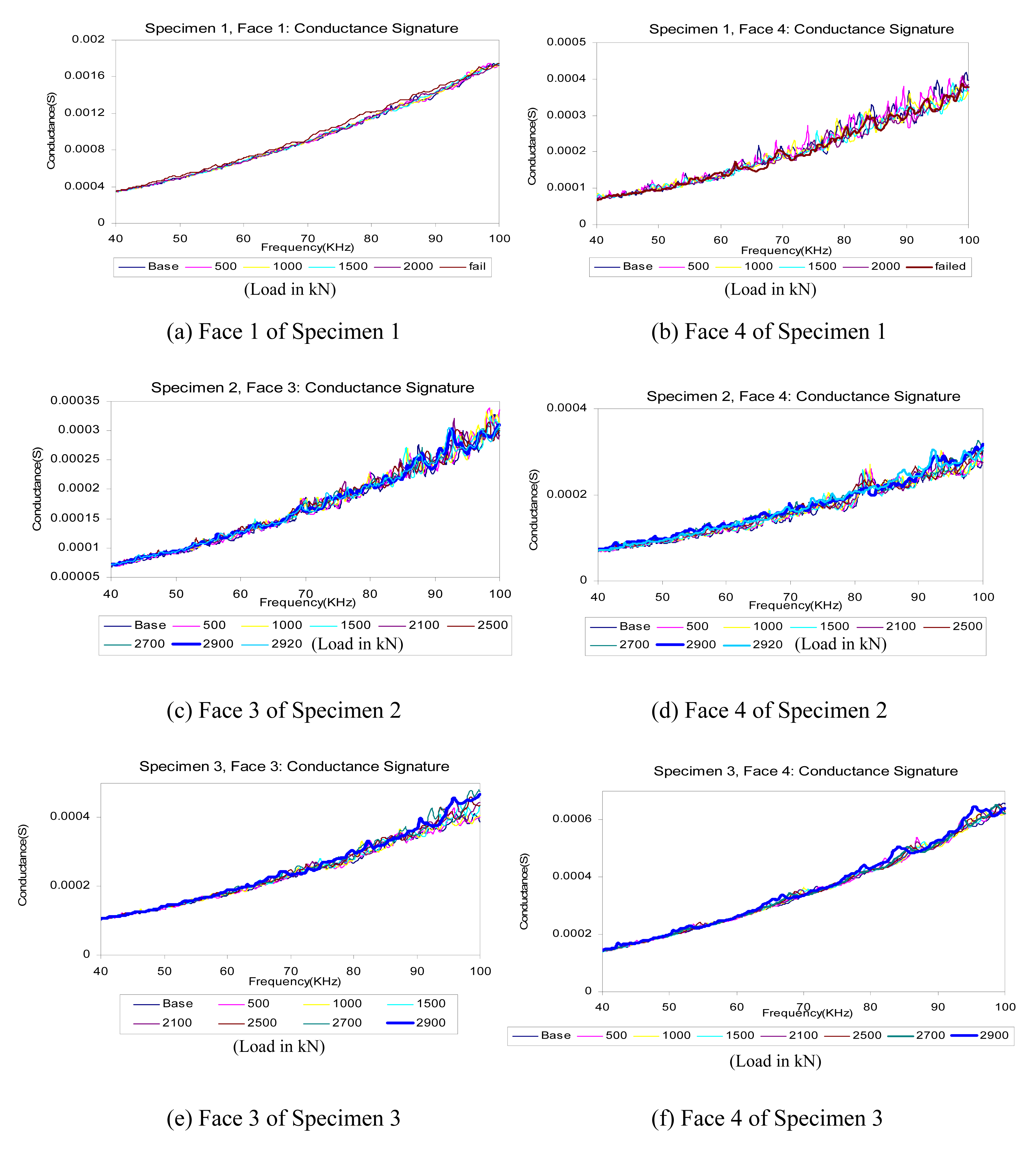
Figure 9 shows the typical experimental conductance signatures for the three test specimens. Figures 9(a,b), (c,d) and (e,f) show the signatures recorded until failure of Specimens 1, 2 and 3, respectively. The respective failure loads are 2765 kN, 2920 kN and 2900 kN. The damage level in the specimens can be assessed by using the root mean square deviation (RMSD). The RMSD values calculated from the conductance signatures for all the faces of Specimens 1, 2 and 3 are shown in Figure 10. Figure 10(a) shows that for Specimen 1, Face 1 was the last to fail because its RMSD value is the smallest as compared to Faces 2, 3 and 4. In fact, it was observed from the RMSD indices that the order of failures should be Face 2 first, followd by Faces 3, 4 and 1. This is in accordance with the experimental observation. Similarly, the variations for the RMSD values of Specimens 2 and 3 also matched the experimental observations. The above experimental results indicates that based on the PZT conductance signatures, the RMSD index could be a good indicator for failure sequence in rocks. Further research work is desirable to confirm this finding.
4.3 Extraction of structural mechanical impedance from admittance signature
The above damage assessment using the RMSD index was based on the raw PZT admittance signature. An alternative is to use the mechnical impedance of the host structure rather than the PZT admittance [18]. The structural mechanical impedance is expected to give more accurate damage information because it excludes the influence of PZT properties on the admittance signature. The following derivation illustrates the procedure of extracting the structural mechanical impedance from the PZT admittance.
The complex mechanical impedances of the host structure and the PZT patch in Eqn.(3) can be written as
where xa and ya are the real and imaginary parts of the mechanical impedance of the PZT patch, respectively; and x and y the real and imaginary parts of the structural mechnical impedance, respectively.
Substituting Eqns. (4) and (5) into (3) and solving the complex Equation (3), we can obtain
where
where r and t can be obtained from the following equation
and GA and BA can be obtained from
Following this computational procedure, the structural mechanical impedance can be extracted from the measured admittance signature of the PZT patch. In this computation, r and t must be calculated precisely from Eqn.(11) using the complex algebra. In addition, PZT mechanical impedance za (or xa and ya) needs to be determined from the experimental test by recording the signature of a PZT patch in the free-free condition.
Taking Face 1 of Specimen 1 as an example, the structural mechanical impedance (real part x and imaginary part y) is extracted from the PZT admittance signature, as plotted in Figure 11. A close look at Figure 11 indicates that the dynamic behaviour of this face is similar to that of a system with parallelly connected spring and damper, for which the following relations hold true [28]
Hence, solving Eqn. (13), system parameters k and c can be derived at any frequency as
In practice, parameter k which represents the stiffness of the structure is of more interest and will be used for damage assessment in the next section. The average value of k over different load cycles is plotted in Figure 11.
4.4 Calibration of PZT patch for damage assessment
Bhalla [29] presented an impedance based damage model for concrete based on the identified stiffness parameter k. At the jth frequency, a damage variable, Dj, can be defined in terms of the identified stiffness as
where koj is the equivalent spring stiffness at the jth measurement point in the pristine state and kdj represents the corresponding value after damage. Thus, Dj is expected to increase in magnitude with damage severity. From the theory of continuum damage mechanics, an element can be deemed to fail if D > Dc, where Dc is the critical value of damage variable. However, it is not possible to define a unique value of Dc due to the unavoidable uncertainties related to rock and PZT patches. Therefore, it is proposed to define the critical value of the damage variable using the theory of fuzzy sets.
The formulation given in Eqn. (16) has an inherent assumption that does not take into account the type of material being analyzed. Additionally, it is assumed that after the occurrence of damage in the structure, the stiffness at each frequency will reduce with respect to the baseline. Again taking Face 1 of Specimen 1 as an example, it is obvious from Figure 12, the plot of stiffness against frequency that stiffness does not necessarily reduce unilaterally as the load increases. In addition, this trend can be observed in all the three specimens. One reasonable explanation for this could be that the stiffness calculated at different actuation frequencies differs, some more sensitive than other, resulting in non-uniform change of the stiffness values for different load cycles. Thus, a slightly modified version of Eqn. (16) can be given as
where the minimum of the ratio between the post-damaged stiffness and the baseline stiffness can be used to compute the damage index. This is to reflect that the stiffness values will tend to decrease as the loading increases until the failure of the specimen.
Using the fuzzy set theory, a fuzzy region may be defined in the interval (DL, DU) where DL and DU respectively represent the lower and the upper limits of the fuzzy region [30,31]. D > DU represents a failure region with 100% failure possibility and D < DL represents a safe region with 0% failure possibility. In the fuzzy region, the failure possibility could vary between 0% and 100%. A characteristic or a membership function fm could be defined (0<fm(D)<1) to express the grade of failure. The fuzzy failure probability (FFP) can then be determined as [31]
where p(D) is the probability density function of damage variable D, which in the present case complies with normal distribution. Based on the experimental observations, DL and DU were chosen as 0.0 and 0.12 respectively. Further, the sinusoidal membership function as given by the following equation was adopted.
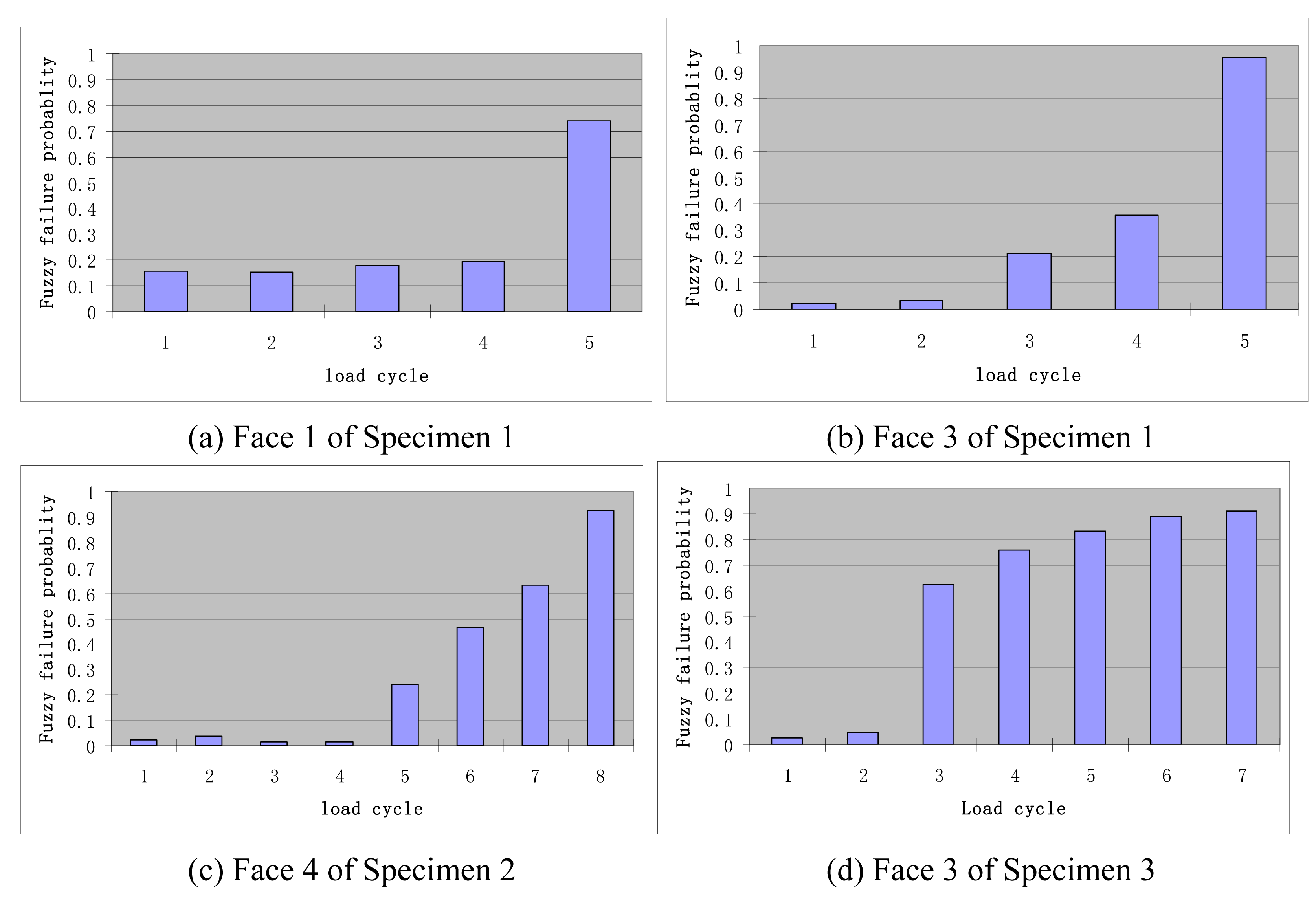
From practical experience, it has been observed that the damage variable typically follows the trend of an S-curve, i.e. initially rising steeply with damage progression and then attaining saturation. This is represented very well by the sinusoidal membership function. Making use of this membership function, the FFP was worked out for the specimens at each load ratio. A load ratio, defined as the ratio between the current load and the failure load, of 0.7 can be regarded as severe damage since the specimens are under near ‘ultimate loads’. For this load ratio, the specimens exhibited a FFP of greater than 70%.
Figure 13 shows the FFP results of each specimen at various test stages. From observations during the tests on rock specimens, following FFP-based classification of damage was recommended.
| (1) FFP < 30% | Incipient damage (Micro-cracks) |
| (2) 30% < FFP < 50% | Moderate damage (Cracks opening up) |
| (3) 50% < FFP < 70% | Severe damage (large visible cracks) |
| (4) FFP > 70% | Failure imminent |
Thus, the fuzzy probabilistic approach quantifies the extent of damage on a uniform 0-100% scale, which can be employed to evaluate damage in real-life rock structures. From these results, it can be found that the EMI method can produce the reasonable FFP for the specimen during the test, and the results can give warning before the structure damaged, showing its potential for practical applications.
5. Conclusion
An SHM scheme was established by using different types of sensors on rock specimens. Different types of sensors offer redundancy in the monitoring system, which is very important in keeping the system functioning even when some of the sensors fail during their service life. In addition, the risk of having total breakdown of the monitoring system due to the failure of one instrument is reduced. From the study, the complementary nature of FBG and PZT smart sensors is shown to be valuable in a comprehensive SHM system, especially for underground structures, where the environment is generally harsh and hazardous. Additionally, if the structural material is non-homogeneous like granite having a number of different chemical constituent with natural faults and cracks, it may take more time for monitoring using conventional sensors like ESGs. The strain measurement can be achieved by the use of FBG sensors with ease. Similarly, other valuable structural information can be gleaned from the PZT signatures. The combination of smart FBG and PZT sensors provides a promising alternative for practical SHM applications.
References and Notes
- Sumitro, S.; Tominaga, M.; Kato, Y. Monitoring Based Maintenance for Long Span Bridges. Presented on First International Conference on Bridge Maintenance, Safety and Management, Barcelona, Spain, 14- 17 July, 2002.
- Bhalla, S.; Yang, Y.W.; Zhao, J.; Soh, C.K. Structural Health Monitoring of Underground Facilities – Technological Issues and Challenges. Tunnelling and Underground Space Technology 2006, 20, 487–500. [Google Scholar]
- Ayres, J.W.; Lalande, F.; Chaudhry, Z.; Rogers, C.A. Qualitative Impedance-Based Health Monitoring of Civil Infrastructures. Smart Materials and Structures 1998, 7, 599–605. [Google Scholar]
- Xu, J.F.; Yang, Y.W.; Soh, C.K. Electromechanical Impedance-Based Structural Health Monitoring with Evolutionary Programming. Journal of Aerospace Engineering 2004, 17, 182–193. [Google Scholar]
- Hill, K.O.; Fujii, Y.; Johnson, D.C.; Kawasaki, B.S. Photosensitivity in Optical Fiber Waveguides: Application to Reflection Filter Fabrication. Applied Physics Letters 1978, 32, 647–649. [Google Scholar]
- Meltz, G.; Morey, W.W.; Glenn, W.H. Formation of Bragg Gratings in Optical Fibers by a Transverse Holographic Method. Optics Letters 1989, 14, 823–825. [Google Scholar]
- Maaskant, R.; Alaie, A.T.; Measures, R.M.; Tadros, G.; Rizkalls, S.H.; Guha-Thakurta, A. Fiber-Optic Bragg Grating Sensors for Bridge Monitoring. Cement and Concrete Composites 1997, 19, 21–33. [Google Scholar]
- Todd, M.D.; Johnson, G.A.; Vohra, S.T. Deployment of Fiber Bragg Grating-Based Measurement System in a Structural Health Monitoring Application. Smart Materials and Structures 2001, 10, 534–539. [Google Scholar]
- Moyo, P.; Brownjohn, J.M.W.; Suresh, R.; Tjin, S.C. Development of Fibre Bragg Grating Sensors for Monitoring Civil Infrastructure. Engineering Structures 2005, 27, 1828–1834. [Google Scholar]
- Kersey, A.D.; Davis, M.A.; Patrick, H.J. Fiber Grating Sensor. Journal of Lightwave Technology 1997, 15, 1442–1461. [Google Scholar]
- Sun, F.P.; Chaudhry, Z.; Rogers, C.A.; Majmundar, M.; Liang, C. Automated Real-Time Structural Health Monitoring via Signature Pattern Recognition. Proceedings of SPIE 1995, 2443, 236–247. [Google Scholar]
- Yang, Y.W.; Xu, J.F.; Soh, C.K. Generic Impedance-Based Model for Structure-Piezoceramic Interacting System. J of Aerospace Engineering 2005, 18, 93–101. [Google Scholar]
- Liang, C.; Sun, F.P.; Rogers, C.A. Coupled Electro-Mechanical Analysis of Adaptive Material Systems - Determination of the Actuator Power Consumption and System Energy Transfer. Journal of Intelligent Material Systems and Structures 1994, 5, 12–20. [Google Scholar]
- Zhou, S.; Liang, C.; Rogers, C.A. An Impedance-Based System Modeling Approach for Induced Strain Actuator-Driven Structures. Journal of Vibration and Acoustics 1996, 118, 323–331. [Google Scholar]
- Annamdas, V.G.M.; Yang, Y.W.; Soh, C.K. Influence of Loading on Electromechanical Admittance of Piezoceramic Transducers. Smart Materials and Structures 2007, 16, 1888–1897. [Google Scholar]
- Yang, Y.W.; Hu, Y.H. Electromechanical Impedance Modeling of PZT Transducers for Health Monitoring of Cylindrical Shell Structures. Smart Materials and Structures 2008, 17, 015005. [Google Scholar]
- Hu, Y.H.; Yang, Y.W. Wave Propagation Modeling of PZT Sensing Region for Structural Health Monitoring. Smart Materials and Structures 2007, 16, 706–716. [Google Scholar]
- Yang, Y.W.; Hu, Y.H.; Lu, Y. Sensitivity of PZT Impedance Sensors for Damage Dection of Concrete Structures. Sensors 2008, 8, 327–346. [Google Scholar]
- Park, G.; Cudney, H.H.; Inman, D.J. Impedance-Based Health Monitoring of Civil Structural Components. Journal of Infrastructure Systems 2000, 6, 153–160. [Google Scholar]
- Park, G.; Cudney, H.H.; Inman, D.J. Feasibility of Using Impedance-Based Damage Assessment for Pipeline Structures. Earthquake Engineering and Structural Dynamics 2001, 30, 1463–1474. [Google Scholar]
- Giurgiutiu, V.; Zagrai, A.N. Embedded Self-Sensing Piezoelectric Sensors for On-Line Structural Identification. Journal of Vibration and Acoustics 2002, 124, 116–125. [Google Scholar]
- Micron Optics. http://www.micronoptics.com/.
- Tokyo Sokki Kenkyujo Co. Ltd. TML Products Guide; Tokyo, Japan, 2004. [Google Scholar]
- PI Ceramic. http://www.piceramic.de.
- SiF Universal. http://sif-u.com/.
- RS Components. http://www.rs-componenets.com.
- Huntsman Advanced Materials. http://www.adhesives.vantico.com/.
- Hixon, E.L. Mechanical Impedance. In Shock and Vibration Handbook, 3rd edition; Harris, C.M., Ed.; McGraw Hill: New York, 1988; pp. 10.1–10.46. [Google Scholar]
- Bhalla, S. A Mechanical Impedance Approach for Structural Identification, Health Monitoring and Non-Destructive Evaluation Using Piezo-Impedance Transducer. PhD Thesis, Nanyang Technological University, Singapore, 2004. [Google Scholar]
- Valliappan, S.; Pham, T.D. Fuzzy Finite Element Analysis of a Foundation on an Elastic Medium. International Journal for Numerical and Analytical Methods on Geomechanics 1993, 17, 771–789. [Google Scholar]
- Wu, C.Q.; Hao, H.; Zhou, Y.X. Fuzzy-Random Probabilistic Analysis of Rock Mass Responses to Explosive Loads. Computers and Geotechnics 1999, 25, 205–225. [Google Scholar]
Figure 1.
Principle of FBG sensors.
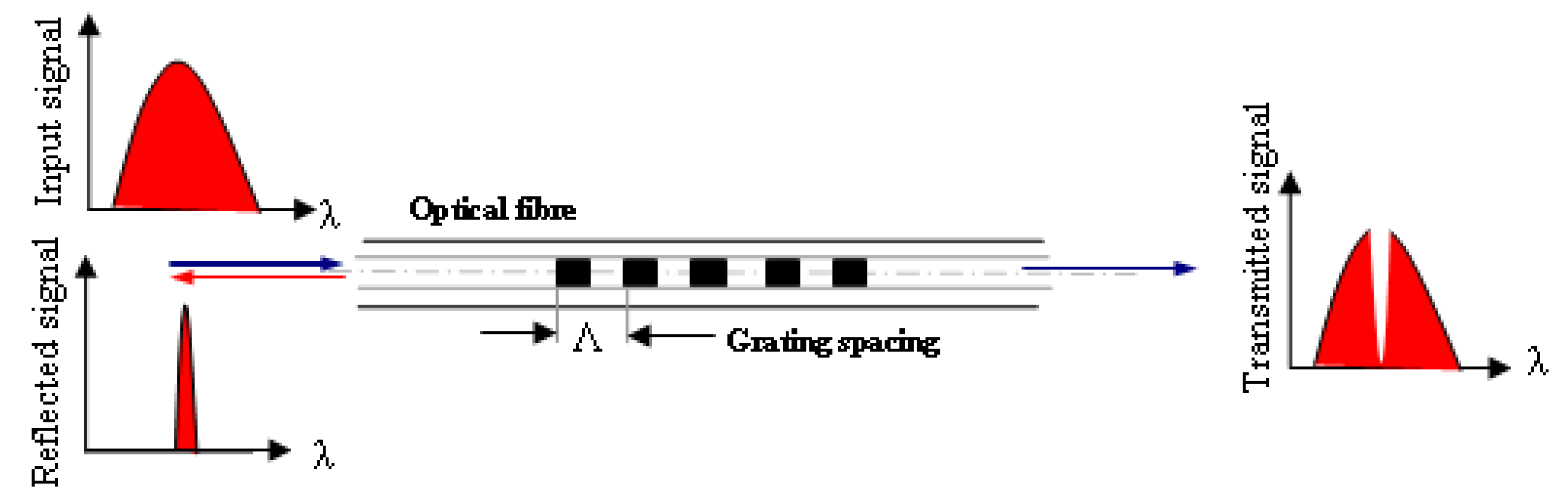
Figure 2.
Experimental equipments.

Figure 3.
A specimen with PZT, FBG and ESG sensors installed.
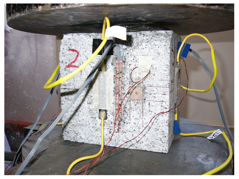
Figure 4.
Locations of ESG, FBG and PZT sensors on rock specimen.
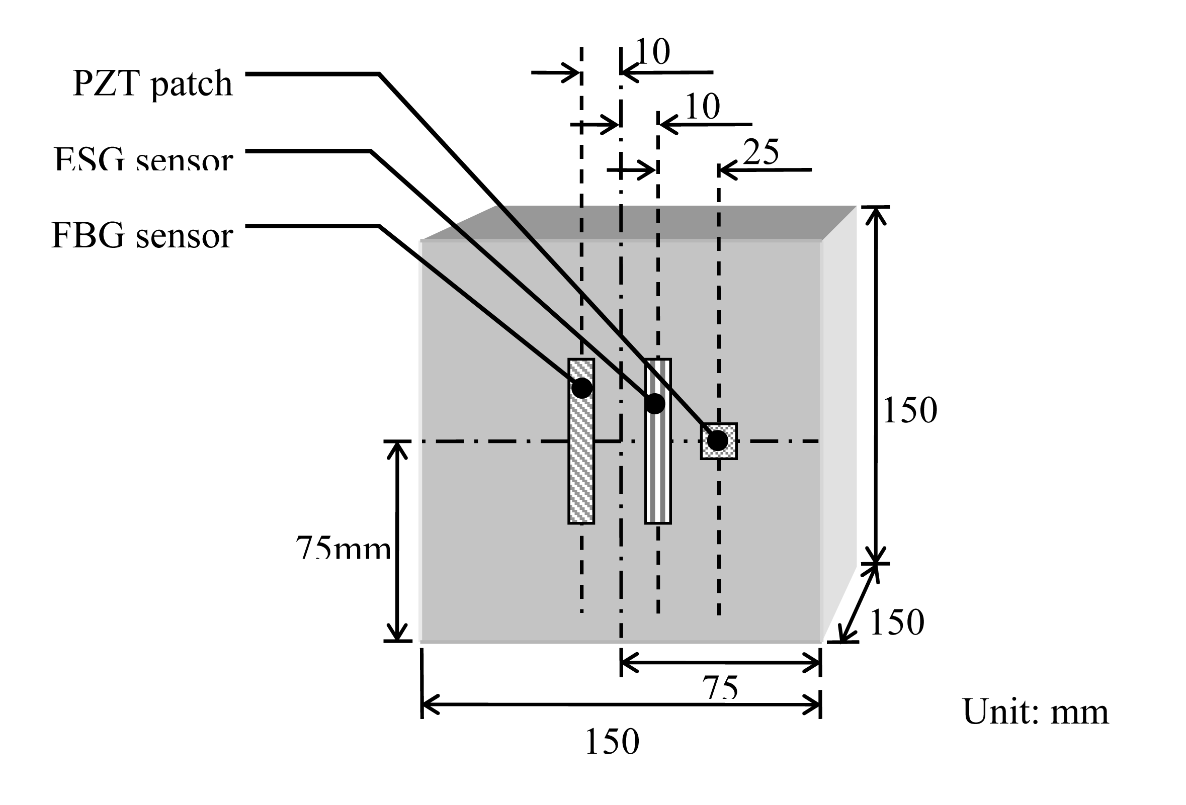
Figure 5.
Comparison of stress-strain relationship measured by ESG and FBG sensors on Specimen 1.
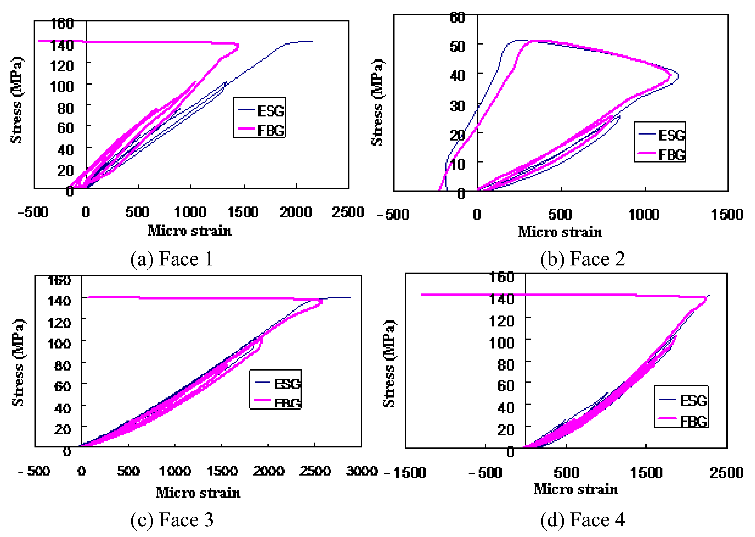
Figure 6.
Comparison of stress-strain relationship measured by ESG and FBG sensors on Specimen 2.

Figure 7.
Comparison of stress-strain relationship measured by ESG and FBG sensors on Specimen 3.

Figure 8.
Specimen 2 after failure (Face 1 being sheared off).
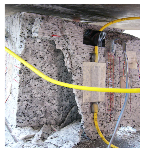
Figure 9.
Conductance signatures of PZT sensors at various loading stages.

Figure 10.
RMSD variations of conductance for all specimens.

Figure 11.
Plot of extracted mechanical impedance (x and y) and equivalent stiffness

Figure 12.
A comparison of stiffness at various frequencies for different load cycles.
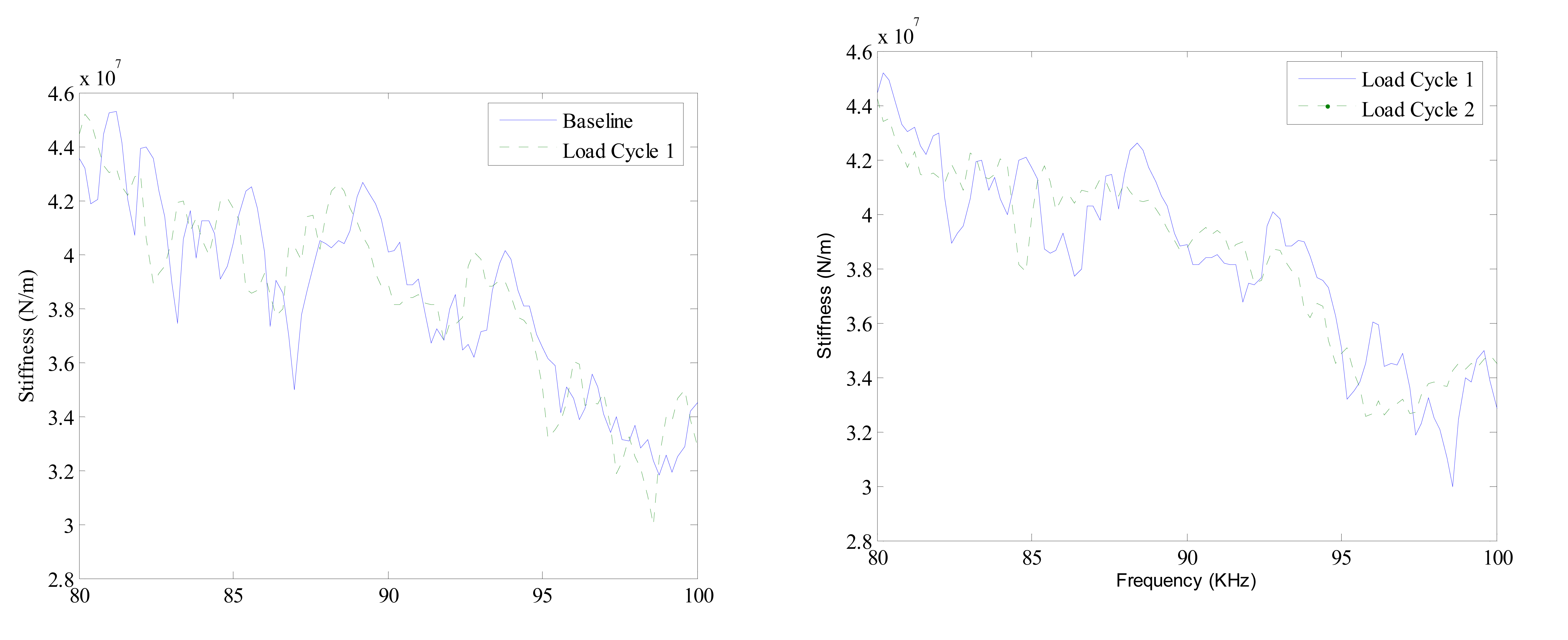
Figure 13.
Fuzzy failure probability for different specimens.

| Load Cycle Number | Maximum Load (KN) | Strain measurement interval (KN) |
|---|---|---|
| 1 | 500 | 100 |
| 2 | 1000 | 200 |
| 3 | 1500 | 300 |
| 4 | 2000 | 300 |
| 5 | 2500 | 300 |
| 6 | 2700 | 300 |
| 7 | 2900 | 300 |
| 8 | 2950 | 300 |
© 2008 by MDPI Reproduction is permitted for noncommercial purposes.
Share and Cite
MDPI and ACS Style
Yang, Y.; Annamdas, V.G.M.; Wang, C.; Zhou, Y. Application of Multiplexed FBG and PZT Impedance Sensors for Health Monitoring of Rocks. Sensors 2008, 8, 271-289. https://doi.org/10.3390/s8010271
AMA Style
Yang Y, Annamdas VGM, Wang C, Zhou Y. Application of Multiplexed FBG and PZT Impedance Sensors for Health Monitoring of Rocks. Sensors. 2008; 8(1):271-289. https://doi.org/10.3390/s8010271
Chicago/Turabian StyleYang, Yaowen, Venu Gopal Madhav Annamdas, Chao Wang, and Yingxin Zhou. 2008. "Application of Multiplexed FBG and PZT Impedance Sensors for Health Monitoring of Rocks" Sensors 8, no. 1: 271-289. https://doi.org/10.3390/s8010271