Spatially Explicit Large Area Biomass Estimation: Three Approaches Using Forest Inventory and Remotely Sensed Imagery in a GIS

Abstract

Forest inventory data often provide the required base data to enable the large area mapping of biomass over a range of scales. However, spatially explicit estimates of above-ground biomass (AGB) over large areas may be limited by the spatial extent of the forest inventory relative to the area of interest (i.e., inventories not spatially exhaustive), or by the omission of inventory attributes required for biomass estimation. These spatial and attributional gaps in the forest inventory may result in an underestimation of large area AGB. The continuous nature and synoptic coverage of remotely sensed data have led to their increased application for AGB estimation over large areas, although the use of these data remains challenging in complex forest environments. In this paper, we present an approach to generating spatially explicit estimates of large area AGB by integrating AGB estimates from multiple data sources; 1. using a lookup table of conversion factors applied to a non-spatially exhaustive forest inventory dataset (R² = 0.64; RMSE = 16.95 t/ha), 2. applying a lookup table to unique combinations of land cover and vegetation density outputs derived from remotely sensed data (R² = 0.52; RMSE = 19.97 t/ha), and 3. hybrid mapping by augmenting forest inventory AGB estimates with remotely sensed AGB estimates where there are spatial or attributional gaps in the forest inventory data. Over our 714,852 ha study area in central Saskatchewan, Canada, the AGB estimate generated from the forest inventory was approximately 40 Mega tonnes (Mt); however, the inventory estimate represents only 51% of the total study area. The AGB estimate generated from the remotely sensed outputs that overlap those made from the forest inventory based approach differ by only 2 %; however in total, the remotely sensed estimate is 30 % greater (58 Mt) than the estimate generated from the forest inventory when the entire study area is accounted for. Finally, using the hybrid approach, whereby the remotely sensed inputs were used to fill spatial gaps in the forest inventory, the total AGB for the study area was estimated at 62 Mt. In the example presented, data integration facilitates comprehensive and spatially explicit estimation of AGB for the entire study area.

1. Introduction

Forest biomass is defined by [1] as the above-ground portion of live trees per unit area. In addition to widespread use in carbon budget models [2, 3, 4, 5, 6], biomass estimates are important for a broad range of applications, including: characterizing forest conditions and processes [7, 8, 9, 10]; estimating forest productivity [11, 12, 13, 14]; modeling impacts of fire and other disturbances [15, 16, 17, 18]; and, for modeling the environmental and economic consequences of energy production from biomass [19, 20, 21, 22]. Monitoring changes to biomass over time has also emerged as an important activity for many of these aforementioned applications [23, 24, 25].

Biomass estimates may range from local to global scales, and for some regions, particularly tropical forest regions, there are large variations in the estimates reported in the literature [5, 26, 27, 28, 29]. Global and national estimates of forest above-ground biomass (AGB) are often aspatial estimates, compiled through the tabular generalization of national level forest inventory data [1, 30, 31, 32, 33, 34, 35, 6]. Methods and data sources for generating spatially explicit large-area AGB estimates have been the subject of extensive research [8, 25, 28, 36, 37, 38, 39].

1.1 Biomass Estimation Methods

A variety of approaches and data sources have been used to estimate forest above ground biomass (AGB). A comprehensive review of remote sensing-based estimates of AGB has been completed, categorized by data source: (i) field measurement; (ii) remotely sensed data; or (iii) ancillary data used in GIS-based modeling [40]. Estimation from field measurements may entail destructive sampling [21, 41] or direct measurement [42] and the application of allometric equations [43, 44, 45]. Allometric equations estimate biomass by regressing a measured sample of biomass against tree variables that are easy to measure in the field (e.g., diameter at breast height, height). 607 different equations have been identified in the literature for estimating AGB for tree species growing in Europe [46]. Although equations may be species- or site-specific, they are often generalized to represent mixed forest conditions or large spatial areas [11, 47]. Biomass is commonly estimated by applying conversion factors (biomass expansion factors) to tree volume (either derived from field plot measures or forest inventory data) [1, 2, 11, 30, 32, 48]. Relationships between biomass and other inventory attributes (e.g., basal area) [49] have also been reported. The use of existing forest inventory data to map large area tree AGB has been explored [8]; conversion tables were developed to estimate biomass from attributes contained in provincial forest inventory data, including species composition, crown density, and dominant tree height. Guidance on the selection, development, and application of appropriate biomass factors and allometric equations for large-scale biomass estimation was provided [29].

Remotely sensed data have become an important data source for biomass estimation. The remotely sensed data types and approaches used for biomass estimation have been summarized [40, 50]. Generally, biomass is either estimated via a direct relationship between spectral response and biomass using multiple regression analysis [51], k-nearest neighbor [52], neural networks [53], or through indirect relationships, whereby attributes estimated from the remotely sensed data, such as leaf area index (LAI), structure (crown closure and height) or shadow fraction are used in equations to estimate biomass [12, 36, 38, 54, 55, 56]. Four different remotely sensed methods for AGB estimation were compared for a test area in western Newfoundland and the relative advantages of the different approaches were assessed, concluding that the choice of method depends on the required level of precision and the availability of plot data [57]. Some methods, such as k-nearest neighbor require representative image-specific plot data, whereas other methods are more appropriate when scene-specific plot data are limited [36].

A variety of remotely sensed data sources continue to be employed for biomass mapping including coarse spatial resolution data such as SPOT-VEGETATION and AVHRR [25, 58] and MODIS [12, 47, 59, 60, 61]. To facilitate the linkage of detailed ground measurements to coarse spatial resolution remotely sensed data (e.g., MODIS, AVHRR, IRS-WiFS), several studies have integrated multi-scale imagery into their biomass estimation methodology and incorporated moderate spatial resolution imagery (e.g., Landsat, ASTER) as an intermediary data source between the field data and coarser imagery [52, 60, 62, 63]. Research has demonstrated that it is more effective to generate relationships between field measures and moderate spatial resolution remotely sensed data (e.g., Landsat), and then extrapolate these relationships over larger areas using comparable spectral properties from coarser spatial resolution imagery (e.g., MODIS). Following this approach alleviates the difficulty in linking field measures directly to coarse spatial resolution data [40].

Landsat TM and ETM+ data are the most widely used sources of remotely sensed imagery for forest biomass estimation [36, 37, 38, 53, 57, 58, 63,], but data from other moderate spatial resolution sensors have also been used, including ASTER [60] and Hyperion data [64]. Similarly, high spatial resolution data such as QuickBird [56] and IKONOS [65] have been used for forest biomass estimation. Numerous studies have generated stand attributes from LIDAR data, and then used these attributes as input for allometric biomass equations [66, 67, 68, 69, 70]. Other studies have explored the integration of LIDAR and RADAR data for biomass estimation [71, 72, 73].

GIS-based modeling using ancillary data exclusively, such as climate normals, precipitation data, topography, and vegetation zones is another approach to biomass estimation [74, 75]. Some studies have also used geostatistical approaches (i.e., kriging) to generate spatially explicit maps of AGB from field plots [24, 28], or to improve upon existing biomass estimation [76]. More commonly, GIS is used as the mechanism for integrating multiple data sources for biomass estimation (e.g., forest inventory and remotely sensed data) [9, 37, 77, 78]. MODIS, JERS-1, QuickSCAT, SRTM, climate and vegetation data have been combined to model forest AGB in the Amazon Basin [27]. Similarly, a combination of MODIS and ancillary data (precipitation, temperature, and elevation) has been used to model AGB over large areas [59].

The advantage of approaches that incorporate some form of remotely sensed data, is through provision of a synoptic view of the area of interest, thereby capturing the spatial variability in the attributes of interest (e.g., height, crown closure) [63]. The spatial coverage of large area biomass estimates that are constrained by the limited spatial extent of forest inventories may be expanded through the use of remotely sensed data [8]. Similarly, remotely sensed data can be used to fill spatial, attributional, and temporal gaps in forest inventory data, thereby augmenting and enhancing estimates of forest biomass and carbon stocks derived from forest inventory data [79]. Such a hybrid approach is particularly relevant for non-merchantable forests where basic inventory data required for biomass estimation are lacking.

1.2 Biomass: The Canadian Context

As discussed previously, some methods for biomass estimation, such as the k-nearest neighbor rely on the link between ground plots and satellite imagery [80, 81, 82, 83, 84]. Methods such as these are routinely applied in countries where an extensive regional network of field plots is exploited. One of the limitations to using this approach in Canada is the scarcity of ground-based inventory plots. The lack of sufficient and high-quality sample plots has been identified as a major barrier to the development of robust AGB estimates, and to the subsequent validation of these estimates [40]. The total area of forest and other wooded land in Canada covers an estimated 402.1 Mha [85]. Management of these forests is largely under provincial and territorial government jurisdiction, resulting in differences in forest inventory strategies and methods [86]. A new National Forest Inventory program will provide a framework for the provincial and federal governments to harmonize inventory data collection for national reporting purposes [87, 88]. In the interim, since some provinces have limited or outdated plot information, there are merits to developing a method for estimating biomass that does not rely on an extensive network of ground plots. The ability to generate a forest stand map from interpreted aerial photography (the typical inventory scenario in Canada) provides an important source of information for estimating and mapping biomass [89]. Furthermore, data collection over large areas is facilitated by the synoptic coverage of satellite images [90, 91, 92] and may be used as input for models or for mapping forest biophysical attributes [93].

Estimates of forest AGB are required input for Canada's national forest Carbon Monitoring, Accounting and Reporting system [2, 94, 95], designed to fulfill Canada's reporting requirements under the 1997 Kyoto Protocol [23]. The first national-level forest biomass estimate for Canada was compiled from forest inventory data [1] and subsequently updated [32]. Forest AGB is an important attribute in Canada's new National Forest Inventory [87, 88], and national tree AGB biomass equations have been developed [96] and applied [97] to generate regional and national estimates of forest biomass [89].

In Canada, stand level forest inventory data are collected (at the provincial level) to aid foresters with management decisions, the latter of which are largely a function of forest stand volume, by species. Consequently, forest inventory data are structured to provide volume (by species) exclusively for merchantable stands [98]. Merchantable timber is defined as “a tree or stand that has attained sufficient size, quality and/or volume to make it suitable for harvesting” [99]. Only a limited suite of attributes are typically collected (through air photo interpretation) for stands considered non-merchantable or non-productive, and typically, no structural or volume attributes are recorded. As a result, inventory-to-biomass conversion equations cannot be applied to these stands, resulting in spatial gaps in biomass estimates relying on specific attributes in the forest inventory data [8, 32, 89]. In the most recent national estimation of biomass, attributional gaps in forest inventory data (i.e., records with no volume data) were circumvented by either (i) generating missing volumes for merchantable stands using lookup tables of average volume per hectare; and, using lookup tables of average biomass per ha, (ii) driven by ecozone and predominant genus (for treed, non-merchantable stands); or (iii) driven by land cover type (for vegetated, non-treed records). For (ii) and (iii), lookup tables were generated using permanent or temporary sample plot data and published information [97].

1.3 Objective

Given the advantages of using remotely sensed data for AGB estimation, the integration of multi-source data (which includes remotely sensed data) within a GIS is one possible approach to generating spatially explicit estimates of AGB over large areas [40]. The objective of this investigation was to demonstrate how data integration can facilitate spatially explicit AGB estimation over a large area where forest inventory exists but is not spatially exhaustive, and where only a sparse set of field data are available. To achieve this objective, three different approaches to AGB estimation are implemented and reported upon. First, spatially explicit AGB is estimated using forest inventory data that is not spatially or attributionally comprehensive for the study area. Second, spatially explicit AGB for the entire study area is estimated using land cover and vegetation density outputs generated from moderate resolution remotely sensed imagery. Finally, a hybrid approach is followed whereby AGB estimates generated from the forest inventory are augmented with estimates of AGB generated from the remotely sensed data in areas where the forest inventory data has attributional or spatial gaps. The intent is to demonstrate how spatially explicit estimates of biomass may be generated by using the forest inventory data where available, and by filling gaps in these estimates with other data sources in order to provide a complete and spatially explicit representation of biomass resources.

2. Study Area and Data

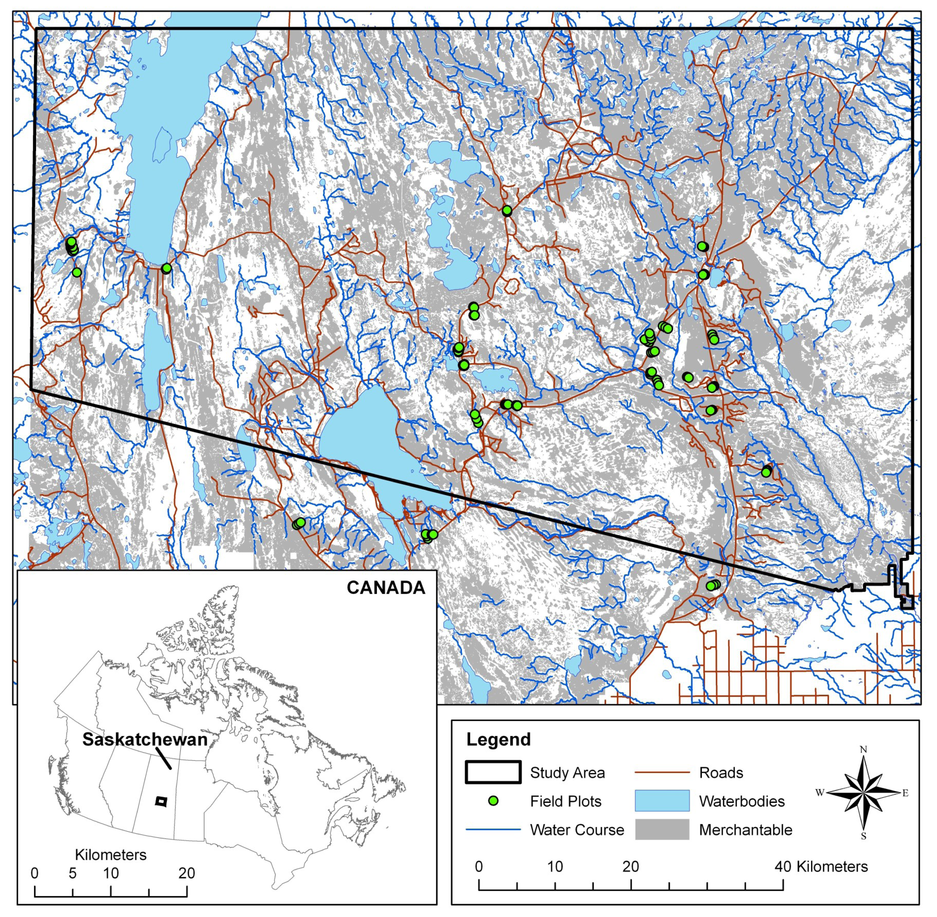
2.1. Study Area

The study area, located in central Saskatchewan, Canada, encompasses approximately 714,852 ha and was selected to represent a variety of boreal forest conditions and species types (Figure 1). Located near the Southern Study Area established as a component of the BOReal Ecosystem Atmosphere Study (BOREAS) [100, 101], the study area is found largely within the boreal plains ecoregion, with a tree species transition from deciduous-dominated mixedwoods in the southern portion, to coniferous-dominated mixedwoods in the northern portion [102, 103]. The area contains mixed boreal forest, composed of aspen (Populus tremuloides) and white spruce (Picea glauca) which are common where the sites are well drained. Jack pine (Pinus banksiana) and black spruce (Picea mariana) are found on dry sites composed of coarse-textured soils. In poorly drained areas, bogs support black spruce and tamarack (Larix laricina). Also present are fen areas, which are composed mostly of sedge vegetation with discontinuous cover of tree species such as tamarack. Forest disturbance is largely the result of localized logging operations and fire. Recent fires have been limited in their spatial extent and frequency through a comprehensive forest fire suppression program [104].

The study area is characterized by a continental climate, with a range of temperature and precipitation conditions found seasonally. For example, monthly precipitation ranges from approximately 19 to 74 mm, between January and July, and constitutes one of the most important limiting factors for ecosystem productivity. Average daily temperature ranges from approximately -22 to 17 °C [105]. The growing season is from March to November and the mean number of growing degree days is 1300 over the range of elevation and latitude within the study area, based upon 1951 to 1980 climate norms [106].

Located within the Saskatchewan Plains Region of the Great Plains Province of North America, the topography of the study area is of gentle relief, with elevations ranging from 400 to 700 m. The dominant landforms consist of glacial till plains, and rolling or hilly moraines. The geomorphological origin of the landforms found in the pilot region are glaciofluvial, glaciolacustrine, fluvial lacustrine, alluvial, and aeolian. As a result, soil development has been upon thick glacial deposits. Soils range from grey wooded to degraded black with brunisolic, gleysolic, chernozemic, luvisolic and organic soil orders [104].

2.2. Field Data

As a component of the BOREAS project [101], forest mensuration data were collected at 130 sample locations during the summer of 1994. Published data describe in detail the plot locations [107], measurement methods, and overstorey characteristics [108]. Trees were considered appropriate for overstorey sampling based upon a height greater than 1.3 m. Point-samples (with a Basal Area Factor ranging from 0.394 to 3 m² ha^-1) or fixed-area plots (ranging in size from 25 to 100 m²) were used for overstory measurements [109]. For each overstorey plot, a number of attributes were collected including DBH, species, canopy class, and health status. For a sub-sample of trees within each plot, representing a range of canopy classes and species, additional attributes were collected including: height, crown diameter, and core samples (for age determination). Understorey measurements used fixed area plots of 4 or 25 m² and percent cover was estimated visually for all species present [109].

Stand basal area and stem density were calculated from these measured data [109]. Volume, or live stem volume, is an estimate of the total volume of wood in tree stems for the stand including the entire stem, not only the merchantable component of the tree as measured for commercial inventory purposes [108]. Tree volumes were calculated from estimated height (or measured height, if available) and measured DBH, multiplied by the number of stems per ha, and summed to estimate total plot volume [109]. Total AGB for each plot was estimated with regression equations [110], which use height, DBH, and species-specific allometric equations to estimate biomass for each tree [109]. In total, 124 of the BOREAS sample plots were available within our study area.

2.3. Forest Inventory Data

The inventory system in Saskatchewan is based upon the interpretation of 1:15,000 stereo aerial photographs, with re-inventory conducted on a 15-year (approximate) cycle [111]. Stereo aerial photographs were collected, interpreted, and digitised into a forest inventory GIS product over a 3.5-year period, starting in 1984 [111]. Delineation of the land base into homogenous units (hereafter referred to as forest inventory polygons) is guided by biophysical criteria that can be recognized and differentiated from the air photos (e.g., species, density, height) [112]. However, our entire study area was not re-inventoried in 1984, resulting in variable vintages for the forest inventory: approximately 8% of the study area was inventoried prior to 1984, 78% in 1984, and the remaining 14% of the study area was inventoried after 1985. The source year of the inventory was used to project dynamic inventory attributes (e.g. age, height, stocking class) to represent a constant base year, and to coincide with the date of field data collection in 1994. The study area contained 8 coniferous, 84 mixedwood, and 7 deciduous species groups. Forest inventory attributes were used in conjunction with provincially developed lookup tables to assign volumes to the merchantable portions of trees within each merchantable stand. There were 79,056 inventory polygons within the study area, of which 50,247 polygons were merchantable (Figure 1), accounting for 365,572 ha, or 51% of the total study area (

Table 1. Forest inventory summary for the study area.

COVER TYPE	NUMBER OFINVENTORYPOLYGONS	AREA (HECTARES)
Merchantable Forest Inventory Polygons (by leading species)
Black Spruce	19,483	109,850
Jack Pine	17,333	158,974
Balsam Fir	3	6
Tamarack	573	3,682
White Spruce	2,219	12,741
Trembling Aspen	10,307	78,191
Balsam Poplar	3	8
Paper Birch	326	2,120
SUB-TOTAL	50,247	365,572
Non-merchantable Forest Inventory Polygons
SUB-TOTAL	28,809	309,081
Non-Inventoried Portion of Study Area
SUB-TOTAL	0	40,199
TOTAL STUDY AREA	79,056	714, 852

).

2.4. Remotely Sensed Data

Landsat TM data were selected for AGB estimation due to its suitability in terms of resolution and practical considerations associated with its use [40]; the spatial resolution of approximately 30 m by 30 m is adequate to assess information at the forest stand level, and this imagery has a minimum mapping area of about 0.5 ha, which is compatible with standard forestry mapping practices [86, 113]. The Landsat TM image, path 37, row 22, acquired July 1994, was georectified using a first-order polynomial rectification, resulting in an RMS error of 0.80 pixels (24m). A top-of-atmosphere correction was applied to convert the image to TOA reflectance [114]. This correction accounts for differences in sensor and viewing geometry, but does not correct for variations in absolute atmospheric conditions.

3. Methods

3.1. Remotely Sensed Image Classification

The Landsat TM image was classified using a hyperclustering and labeling approach with an unsupervised K-means algorithm [95]. The original 241 clusters were manually merged to 16 broad land cover classes (

Table 2. Summary of land cover and density classes estimated from the Landsat TM data.

COVER TYPE	AREA (HECTARES)
Forested Cover Types
Coniferous, Dense	171,604
Coniferous, Open	99,711
Coniferous, Sparse	55,911
Deciduous, Dense	42,357
Deciduous, Open	20,909
Deciduous, Sparse	1,762
Mixed, Dense	99,973
Mixed, Open	16,393
Mixed, Sparse	5,569
SUBTOTAL	514,189
Non-Forested Cover Types
Shrubs	31,819
Wetland Non-Treed	70,694
Non-Treed Herbaceous	16,441
Exposed Land	21,178
High Biomass Cropland	32
Low Biomass Cropland	1,956
Water bodies	58,543
SUBTOTAL	200,663
TOTAL	714,852

). These classes are similar to those defined in Level 4 of the NFI classification schema [115], with the addition of some of the classes used for large area land cover mapping in Canada with AVHRR data (NBIOME), such as low and high biomass croplands [116]. A sample of aerial photography (1:15,000), collected in 1984 for the forest inventory program, was made available by the Saskatchewan government to assist in assigning the spectral clusters to the appropriate land cover classes.

Following [117], a maximum likelihood approach was used to estimate stand density classes (also following NFI defined categories;

Table 3. NFI and corresponding Saskatchewan forest inventory density classes. The forest inventory classes, as defined in Saskatchewan's forest inventory, do not exactly match the NFI density classes. As a result, the forest inventory ranges were reassigned to a NFI category to provide compatibility between the remote sensing and stand map-derived layers, and to enable cross-referencing and estimation.

NFI DENSITY (%)	NFI CLASS	SASKATCHEWAN FOREST INVENTORY DENSITY (%)
61 – 100	Dense	56 – 80; > 81
26 – 60.9	Open	31 – 55
10 – 25.9	Sparse	10 – 30

) for each forest stand type (i.e., coniferous, mixedwood, deciduous) identified from the clustering and labeling of the Landsat TM image, as described above. Training data for the density classes were generated by interpreting the aforementioned air photos for a sample of each forest cover type. With the photo-interpreted crown closures as reference data, the six optical Landsat channels and the variance of Landsat TM channel 4 within a 3 by 3 pixel-window were input into a maximum likelihood classification. The variance texture measure is included to provide forest structural information to augment the spectral data [40]. Each stand type, as identified by the satellite image, was assigned a density class (dense, open, and sparse) using the maximum likelihood approach. Thus, from the remotely sensed data, two pieces of information required for AGB estimation were generated: stand type and stand density.

3.2. Validation of the classified Landsat imagery

Typically, to assess the accuracy of a remotely sensed image classification a source of ground validation data is required. The ground validation sample should capture all classes found in the classification and cover the range of conditions that may be encountered. These types of ground validation data are not always available [118]. The use of the forest inventory data as a validation source is problematic due to the age of the inventory and the methods used to delineate polygons; these factors often result in a poor agreement between data sources [119]. Additionally, within-polygon spectral heterogeneity [120], and the method for selecting a pixel within the polygon for comparison, are confounding issues [119]. The sample plot data collected for the BOREAS study included information on vegetation cover types; hence the field plot data were selected as the best source to validate the Landsat image classification results. Unfortunately, the field plots did not contain information for the mixedwood open and sparse classes, or for any the non-forest classes (Table 2).

3.3. Data Compatibility: Field Data and Remotely Sensed Outputs

In order to make comparisons between the BOREAS field plots and the remotely sensed outputs, the field plots had to be assigned a cover type and a density class matching those used in the image classification procedures (Table 2 and Table 3). Species and stem density information in the field plot data were used to assign each of the field plots a corresponding cover type and density class.

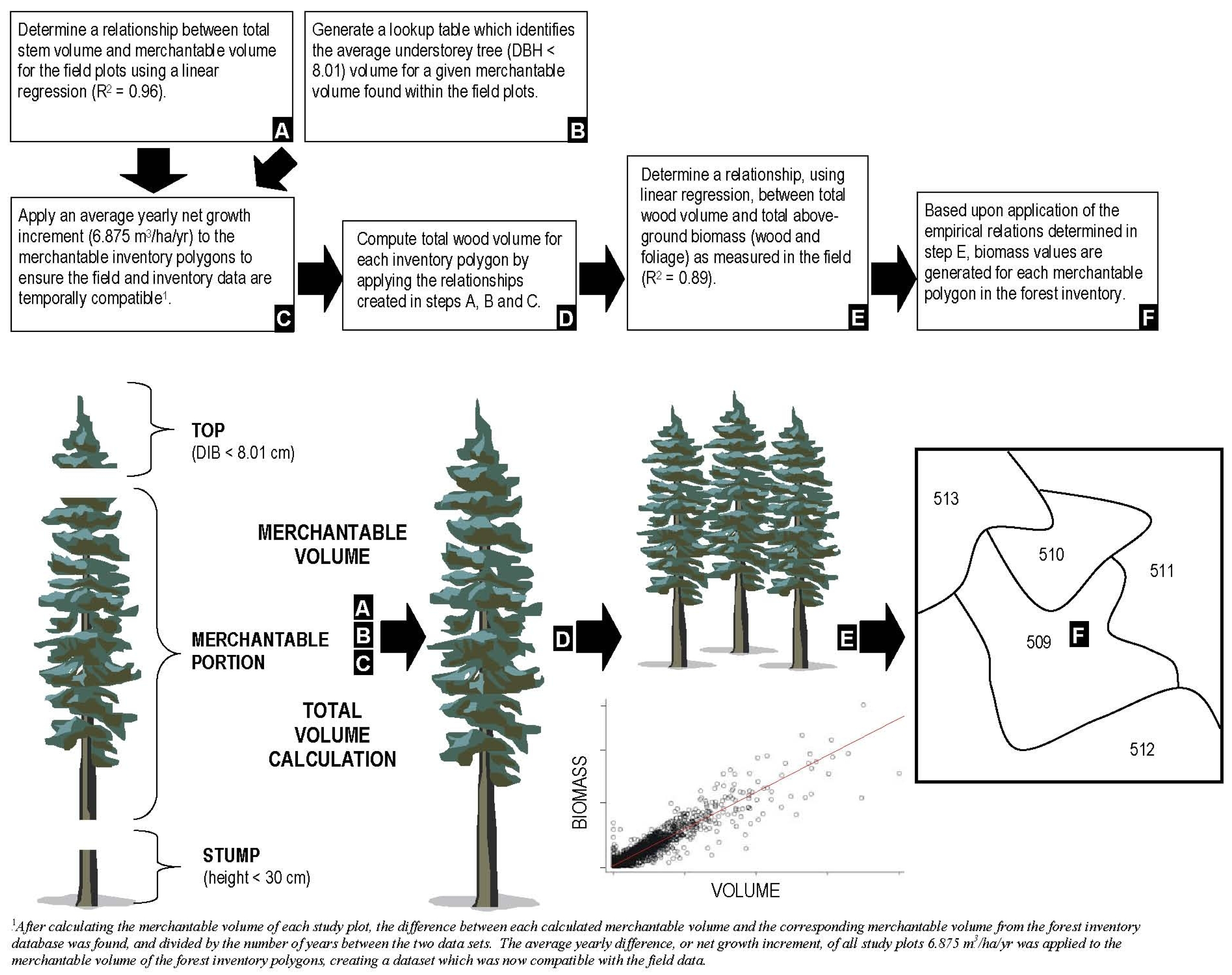
3.4. Data Compatibility: Field Data and Forest Inventory

In order to make comparisons between the field data and the inventory data, including timber volumes from lookup tables provided by the Saskatchewan government, two issues needed to be resolved: (i) the total stem volumes reported in the field data included merchantable and non-merchantable portions of all trees, whereas the volume figures provided in the forest inventory lookup tables included only the merchantable portion of trees with a DBH above the merchantable limit; and (ii), there was an age difference of up to 10 years between the field plot and forest inventory data, an amount of time in which trees can grow enough to markedly change the stand volume.

In accounting for non-merchantable and sub-merchantable timber volume in the forest inventory polygons, it was important first to understand how the total volumes reported for the field plots [108] were calculated. By following the steps outlined in the BOREAS documentation and seeking input from other forest inventory specialists where documentation was incomplete, it was possible to determine how the field volumes were calculated. As tree volumes were predicted using Kozak's variable exponent taper function [121], the key to matching the inventory merchantable volumes with those in [108] was in replicating how this formula was applied. The results in [108] were matched using the following procedure:

• For each of the 3,124 sampled trees, height was calculated as a function of DBH and tree species, using regression equations and parameters listed in [108]. Tree heights were then adjusted using a plot bias multiplier, as described in [108].
• Each tree was divided into ten segments—the stump segment was 30 cm in length, and the remaining nine segments were equal in length, i.e., segment_length= (tree_height-30cm)÷9 and Kozak's formula was used to predict the inside-bark diameter at the top, middle, and bottom of each of these segments. The parameters used for Saskatchewan tree species in Kozak's formula were taken from [122].
• The volume of the stump segment was calculated using the volume formula for a cylinder, and the volume of the top segment was calculated using the volume formula for a cone.
• Newton's formula for volume of a neiloid, cone, or paraboloid frustum [123] was used to calculate the volume of the remaining eight segments.
• The volumes of all segments of each tree were totaled, and the point sampling factors were applied to individual tree volumes to determine the per-hectare volume represented by each tree. Finally, the sum of each of these per-hectare volumes was found, the result being the total live stem volume of the study plot.

After completing this routine for all field plots and achieving results matching those presented in [108] (R² = 0.99) it was possible to move on to calculating the merchantable volume of each tree for the field data. For this study, merchantable volume was defined as the volume of wood in the stem of a tree between the top of the stump (at height = 30 cm), and the height at which the tree diameter inside bark was 8.01 cm. Finding merchantable volume involved the following steps:

• The volume of the stump was first subtracted from the total volume of each tree.
• Kozak's formula was applied in reverse, as described in [121], to determine the merchantable height of each tree, or the height at which the diameter inside bark was approximately 8.01 cm. The formula for volume of a cone was used to calculate the volume of wood above the merchantable height, and this amount was subtracted from the total volume.
• Point sampling factors were applied to the remaining volume of each tree as in step 5 above, and the merchantable stand volume in cubic meters per hectare was totaled for each study plot.

After calculating the merchantable volume of each study plot, the difference between each calculated merchantable volume and the corresponding merchantable volume from the forest inventory database was found, and divided by the number of years between the two data sets. The average yearly difference, or net growth increment, of all study plots was 6.875 m³ha^-1yr^-1 and this factor was applied to the merchantable volume of the forest inventory polygons, creating a dataset which was now compatible with the field data.

The final step in creating a forest inventory dataset which was compatible with the field data was to find the total stem volume of each forest polygon. A model needed to be found which predicted total stem volume by accounting for the sub-merchantable component which was important in stands with lower merchantable volume. In field plots with higher merchantable volume, the relationship of merchantable volume to total volume was nearly one to one. In field plots with lower merchantable volume, the contribution of the smaller trees to the total volume was greater and more variable. It was observed that, in general, the total volume of small trees in each stand was inversely related to merchantable stand volume, and several models predicting the volume of small trees as a function of merchantable stand volume were explored. Finding a curvilinear function which added a small trees component to the total volume proved unsuccessful, and it was finally decided that a lookup table which found the average sub-merchantable tree volume for a given merchantable volume would be adequate.

Predicting total volume by adding together the volume of large trees and the volume of small trees, both as functions of merchantable volume, was achieved in four steps:

• Field plots which fell in a single forest inventory polygon were grouped together, and values for sub-merchantable volume, total volume of big trees, and merchantable volume were averaged for these groups of field plots.
• The average merchantable volumes of the field plot groups were divided into 30 m³/ha classes. The variance and average total volume of small trees in each of these classes was found, and a lookup table to find the average volume of small trees for a given merchantable volume was created (

  Table 4. Average volume of small trees in each merchantable volume category. A lookup table based on these values was used in the total stem volume estimation model.

  VOLM RANGE (m3/ha)	VOLUME OF SMALL TREES (m3/ha)	VOLM RANGE (m3/ha)	VOLUME OF SMALL TREES (m3/ha)
  				0 – 29.9	23.8	180 – 209.9	2.9*
  30 – 59.9	29.7	210 – 239.9	2.6*
  60 – 89.9	42.7	240 – 269.9	2.2
  90 – 119.9	22.1*	270 – 299.9	1.2
  120 – 149.9	12.9*	300 – 329.9	0.6*
  150 – 179.9	3.6	330 +	0.0

  ^*these values were adjusted using the average of next and previous values to produce a smoother relationship between the two variables

  ). The volume of small trees for a given merchantable volume was adjusted in four instances to produce a smoother relationship between the two variables.
• For trees larger than 8.01 cm, linear regression analysis was used to predict the total volume of these big trees as a function of merchantable volume. The model,

  $${\mathit{\text{VOL}}}_B=1.117\cdot {\mathit{\text{VOL}}}_M,$$

  where VOL_B is the volume of big trees, and VOL_M is the merchantable volume, was found to be accurate, with an R² of 0.964.
• Volumes predicted in (2) and (3) above were totaled for each plot to find the total stem volume using:

  $${\mathit{\text{VOL}}}_T={\mathit{\text{VOL}}}_S+1.117\cdot {\mathit{\text{VOL}}}_M,$$

  where VOL_S is the volume of small, sub-merchantable trees from the lookup table (Table 4).

Total stem volumes were computed for each group of plots using the field data and the forest inventory data, and the results were compared. While a 1:1 relationship between the two sets would have been the ideal result, it was known that fundamental differences in the data sets would preclude this from happening (e.g., forest inventory volumes were in discrete classes, as opposed to the continuous values of the field data). Through the steps outlined above, compatible estimates of merchantable volume and total volume were possible from the field data and the forest inventory data.

3.5. Method 1: Biomass estimation from forest inventory

In the BOREAS field data, AGB and total stem volume for each stand were closely related. Figure 2 provides an overview of the process required to estimate biomass for the inventory polygons. The biomass estimation method followed was based upon the development of empirical relationships between the stand volumes assigned to the forest inventory polygons (using methods described above) and volumes from the BOREAS field plots. Of the 124 BOREAS field plots found within our study area, 95 were spatially coincident with the forest inventory polygons. In some cases, multiple field plots were found within a single polygon, or conversely, field plots straddled more than one inventory polygon. In order to build relationships between the plot-level data and the inventory data, weighted averages for field plot volume and biomass were calculated, proportional to the area of the field plot found within the inventory polygon. In total, 52 inventory polygons contained field plots, representing 26 coniferous, 11 deciduous, and 15 mixedwood inventory polygons.

There are two approaches to estimating biomass with the forest inventory data. One method determines the relationship for each structural cover type (i.e., coniferous, deciduous, or mixed) or preferably, each species, individually, and then combines these estimates to obtain an overall estimate of biomass [124]. Alternatively, the relationship between volume and biomass may be determined using a more generic model that encompasses all species or cover types [34, 92]. The former method is more accurate, provided there are sufficient ground samples to develop the appropriate allometric relationships; the latter method may be more practical for large areas of mixed cover types [125].

These two approaches were explored when developing a model to predict biomass using total volume estimates from forest inventory lookup tables. Individual cover types (ICT) models were based on regression relationships between total volume estimates and biomass measurements for each of hardwood, softwood, and mixed forest cover types. An all cover types model (ACT) was based on a single regression relationship between total volume estimates and biomass measurements for all forest cover types. Linear models were used in all cases, as biomass estimates from the non-linear models that were explored may have become unreasonably high for volume estimates greater than those used to calibrate the models.

In developing the ICT model, 52 paired AGB and total stem volume measurements were divided into three groups based on field plot forest cover type (i.e., coniferous, deciduous, mixedwood). Linear regression analysis was performed on the three data sets, and the regression parameters were used to calculate biomass in tonnes per hectare (t/ha) for each forest inventory polygon in the study area, using total volumes derived from lookup table estimates as described earlier in the Methods section.

Table 5. Formulas used to estimate biomass from regression relationships between total stem volume and AGB measured in the BOREAS field plots.

COVER TYPE	EQUATION	R2	RMSE	SAMPLE SIZE (N)
ICT Models
Deciduous	BIOM = 25.3247 + 0.4451 • VOLT	0.947	9.094	11
Coniferous	BIOM = 35.8934 + 0.3529 • VOLT	0.869	14.565	26
Mixedwood	BIOM = 26.3214 + 0.4617 • VOLT	0.934	18.378	15
ACT Model
All	BIOM = 29.2883 + 0.4123 • VOLT	0.892	16.047	52

contains the regression formulas used to estimate biomass for the forest inventory polygons.

After applying each of the models in Table 5 to the inventory polygons, the inventory-based biomass estimates were extracted from each polygon containing a corresponding field based estimate of biomass (n = 52). To determine the validity of the models in Table 5, regression relationships between the inventory-based AGB estimates, and field-based AGB were then found for each cover type.

3.6. Method 2: Biomass estimation from remotely sensed image outputs

The entire study area is contained within one Landsat TM scene, allowing for biomass estimates for the entire study area to be calculated from the combined cover type and density classes output from the image processing (Table 2 and Table 3). For each cover type-density combination, average AGB values for BOREAS field plots were calculated. These average AGB values were then used as AGB lookup values for the corresponding cover type-density combinations from the remotely sensed data. Since not all of the 16 cover type-density combinations listed in Table 2 were represented by the BOREAS field plots, two issues had to be addressed. First, for the forest cover type-density classes not represented by the field plots (mixedwood open and mixedwood sparse), biomass lookup values (in t/ha) were generated from those forest inventory polygons with similar forest cover type-density attributes. For example, to generate the biomass lookup value for mixedwood open, the mean biomass value was calculated from all the forest inventory polygons with a mixed species composition and a stand density between 31 and 55% (Table 3). Second, AGB lookup values were required for the non-forest land cover classes in the classified Landsat scene. Since these classes were not represented by the BOREAS field plots and corresponded (primarily) to the non-merchantable areas of the forest inventory data, appropriate biomass values were obtained through a literature review and consultation with other researchers familiar with specific cover types (Table 2). Once each cover type-density combination had a corresponding biomass value, a lookup table approach was followed to apply a biomass value to each pixel in the classified image. The lookup values for each of the cover types are provided in

Table 6. AGB lookup values used for each cover type.

COVER TYPE	AGB STANDARD (TONNES/HA)
Forested Cover Types
Coniferous, Dense	111
Coniferous, Open	94
Coniferous, Sparse	89
Deciduous, Dense	126
Deciduous, Open	95
Deciduous, Sparse	94
Mixed, Dense	118
Mixed, Open	95 1
Mixed, Sparse	92 1
Non-Forested Cover Types
Shrubs	35 2
Wetland Non-Treed	25 3
Non-Treed Herbaceous	3 4
Exposed Land	0
High Biomass Cropland	6 4
Low Biomass Cropland	3 4
Water bodies	0

¹Not represented in the BOREAS field plots, estimate generated from comparable polygons in the forest inventory.

²Source: [128] Kovda, V.A., 1976. The problem of biological and economic productivity of the earth's land areas. Soviet Geography, 12:6-23. Biomass for chernozem steppe.

³Source: [129] Bazilevich, N.I., L. Ye. Rodzin, and N.N. Rozov. 1971. Geographical aspects of biological productivity. Soviet Geography, 12:293-317. Biomass for Bogs.

⁴Source: Adrian Johnston, pers.comm.; Agriculture and Agrifood Canada, Lethbridge, AB.

.

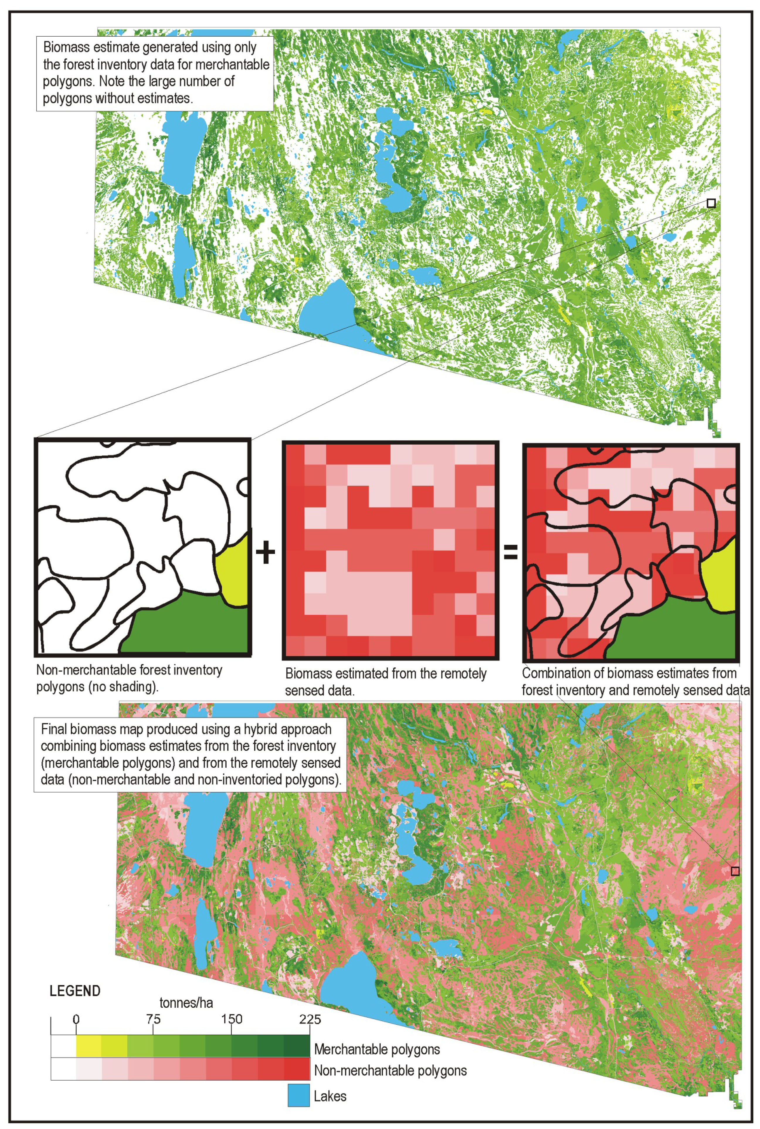
3.7. Method 3: Biomass estimation using a hybrid approach

The hybrid approach integrates the estimates generated from methods 1 and 2 above to create a complete, spatially explicit estimate of AGB for the entire study area. In this approach, spatial and attributional gaps in the forest inventory that preclude an estimation of biomass are filled by estimates generated from the remotely sensed data. In order to facilitate data integration, the non-merchantable forested inventory polygons are populated with the pixel based estimates from the imagery using a polygon decomposition method [126]. Polygon decomposition is the creation of new polygon attribute values by the summation of the pixels found within a given polygon (e.g., summing of all the pixel based biomass values for a polygon based estimate of biomass). This polygon decomposition approach facilitates the harmonization of the forest inventory estimates and the pixel based estimates from the remotely sensed imagery. For those portions of the study area where the forest inventory does not exist, the remotely sensed biomass estimates were used directly. The result is a spatially contiguous representation of biomass across the entire study area.

4. Results and Discussion

Applying the two different biomass estimation approaches (from forest inventory or from remotely sensed imagery) led to three possible approaches to estimate and map biomass in the study area: from the forest inventory exclusively, from remotely sensed image outputs exclusively, and from a hybrid approach where the forest inventory estimates were augmented with remotely sensed image estimates, where the forest inventory had spatial or attributional gaps.

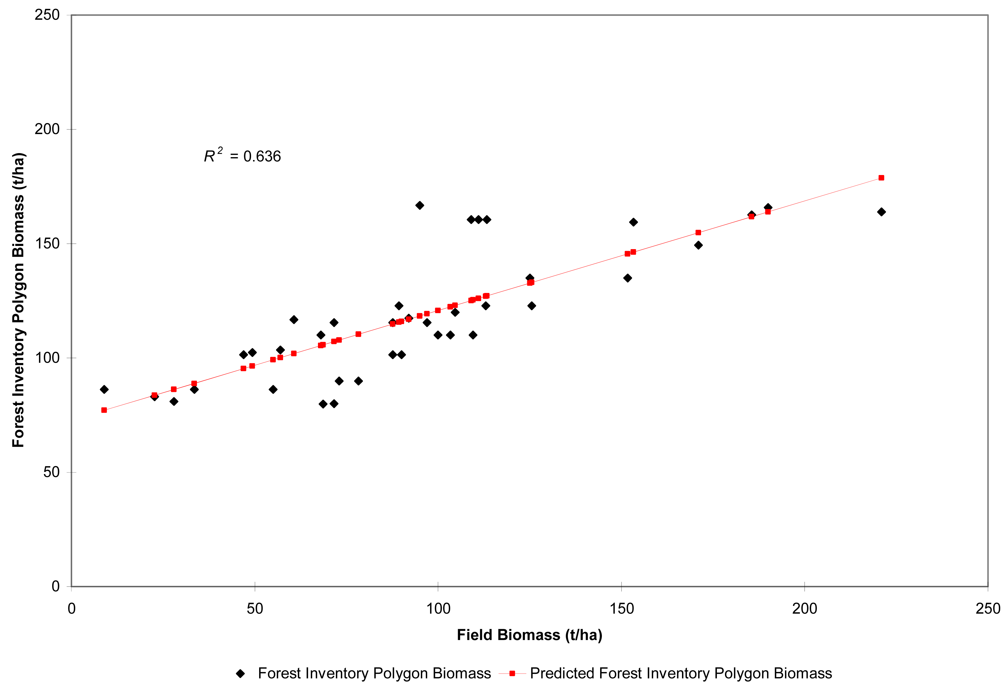
4.1. Method 1: Biomass estimation from forest inventory

After applying each of the models in Table 5 to the inventory polygons, the inventory-based biomass estimates were extracted from each polygon containing a corresponding field based estimate of biomass (n = 52). To determine the validity of the models in Table 5, regression relationships between the inventory-based AGB estimates, and field-based AGB were then found for each cover type. The results of the validation are summarized in

Table 7. Summary of regression statistics for comparisons of field-based biomass versus forest inventory polygon (predicted) AGB estimates.

MODEL	MULTIPLE R	R2	ADJUSTED R2	RMSE	SAMPLE SIZE (N)
ICT Models
Deciduous	0.345	0.119	-0.174	27.629	5
Coniferous	0.639	0.408	0.372	9.643	18
Mixed	0.878	0.771	0.754	21.220	15
ACT Model
All	0.803	0.645	0.636	16.949	38

. The ICT models were shown to be unpredictable, with R² values ranging from −0.174 to 0.754, and were based on too few instances of each cover type. In Figure 3, we present the regression relationship between the predicted and field measured biomass values illustrating a moderate positive relationship between the two estimates, with an R² of 0.64.

The ACT model was applied to all forest inventory polygons in the database, except those classified as non-merchantable. The AGB estimates derived from the forest inventory ranged, by species, from 1 to 209 t/ha. The remaining non-merchantable areas included waterbodies, disturbed land (including burn-overs and cut blocks), and land not inventoried, such as parks or private lands. Total AGB, representing only 51% of the study area, was estimated at approximately 40 Mt (

Table 8. Summary of AGB estimates generated from the forest inventory data.

COVER TYPE	BIOMASS (TONNES)
Merchantable Forest Inventory Polygons (by leading species)
Black Spruce	12,102,414
Jack Pine	15,972,510
Balsam Fir	927
Tamarack	360,509
White Spruce	1,846,504
Trembling Aspen	9,339,950
Balsam Poplar	499
Paper Birch	205,901
SUB-TOTAL	39,829,214
Non-Merchantable Forest Inventory Polygons
SUB-TOTAL	N/A
Non-Inventoried Portion of Study Area
SUB-TOTAL	N/A
TOTAL STUDY AREA	39,829,214

).

4.2. Validation of the classified Landsat imagery

For the forested classes represented in both the field data and the image classification, overall agreement between the assigned cover types was 80.1%. The overall level of agreement between the plot determinations of density and those derived from the Landsat image classification was 73.7%. The BOREAS field data provides an independent data source for validation, as none of the field plots were used for the unsupervised classification of land cover type or in the creation of the supervised maximum likelihood approach for deriving the density information.

4.3. Method 2: Biomass estimation from remotely sensed imagery

The total biomass estimated from the satellite image approach (covering the entire study area) was approximately 58 Mt (

Table 9. Summary of AGB estimates generated from the remotely sensed data.

COVER TYPE	BIOMASS (TONNES)
Forested Cover Types
Coniferous, Dense	19,048,053
Coniferous, Open	9,372,792
Coniferous, Sparse	4,976,068
Deciduous, Dense	5,337,024
Deciduous, Open	1,986,396
Deciduous, Sparse	165,655
Mixed, Dense	11,796,845
Mixed, Open	1,557,340
Mixed, Sparse	512,308
SUB-TOTAL	54,752,480
Non-Forested Cover Types
Shrubs	1,113,657
Wetland Non-Treed	1,767,362
Non-Treed Herbaceous	49,323
Exposed Land	0
High Biomass Cropland	194
Low Biomass Cropland	5,868
Water bodies	0
SUB-TOTAL	2,936,404
TOTAL STUDY AREA	57,688,884

). A regression of the remotely sensed estimates of AGB against the field measured biomass values resulted in an R² of 0.54 (Figure 4).

4.4. Method 3: Biomass estimation using a hybrid approach

Table 10. Using the hybrid approach for AGB estimation, estimates from Method 1 (forest inventory) and Method 2 (remotely sensed outputs) have been integrated to produce a spatially explicit estimate of biomass for the entire study area.

FORESTINVENTORYPOLYGONSTATUS	NUMBER OF INVENTORY POLYGONS	AREA (HECTARES)	METHOD 1FOREST INVENTORY	METHOD 2REMOTELYSENSEDDATA	METHOD 3DATAINTEGRATION
			AGB (TONNES)	AGB (TONNES)	AGB (TONNES)
			Merchantable	50,247	365,572	39,829,214	37,748,175	39,829,214
			Non-merchantable	28,809	309,081	N/A	19,940,709	19,940,709
Not inventoried	0	40,199	N/A	2,593,484	2,593,484
TOTAL	79,056	714,852	39,829,214	57,688,884	62,363,407

summarizes the results of the hybrid or integrated approach to generating an estimate of AGB for the entire study area. Biomass estimates for the non-merchantable classes from method 2 were decomposed to populate the non-merchantable polygons in the forest inventory. Similarly, those portions of the study area where there was no forest inventory data were infilled with the remotely sensed biomass estimates (Figure 5). Total biomass for the merchantable polygons is the same as for the inventory-exclusive approach (Table 8); total biomass for non-merchantable polygons and non-inventoried areas are generated from the remotely sensed data approach (Table 9). Total AGB for the study area was estimated at approximately 62 Mt.

The AGB estimated for the merchantable polygons with Method 2 was 5% lower than the AGB estimated from Method 1. This underestimation of forest biomass by remote sensing methods is a phenomena originally identified by [127]. Other studies have found a saturation effect, particularly in complex forest stands in tropical forests, whereby canopy reflectance becomes saturated when AGB approaches a certain level, and this effect, combined with the impact of canopy shadows, limits the ability of the data for detection of additional biomass beyond that level [40]. Given the capability for and the diligence with which the field and inventory data could be harmonized for this study, and the subsequent volume-biomass associations developed, it is not surprising that the there is a stronger positive relationship between the field and inventory estimates of AGB, when compared to the relationship between the field and remotely sensed estimates of AGB.

The robustness of the inventory estimates of AGB are a function of the photo interpretation, the volume tables generated, and the volume to biomass conversion. Similarly, the robustness of the remote sensing estimates must be considered as a function of the land cover classification, the density estimation approach, and the AGB lookup values applied. As common to most studies using GPS under a forest canopy, both approaches will be impacted by the positional accuracy of the field plot locations. Potential users of the AGB estimates must consider the factors influencing the accuracy of the approach used when applying the results.

For this study, the estimates generated from the forest inventory, where available, are assumed to be more robust than those generated from the remotely sensed outputs. As a result, we treat the inventory estimates of AGB as the best available estimates, and then augment these estimates where there are spatial or attributional gaps in the forest inventory. By integrating multiple data sources, we are able to generate a complete picture of AGB for the study area. If we had relied only on the estimate generated from the forest inventory, we would have underestimated total AGB for the study area by 20% because the inventory only provided estimates for 51% of the study area. By integrating the AGB estimates from the two approaches, we are able to generate a more complete estimate representing 100% of the study area. Equally important is the ability to generate a map of AGB in the study area, thereby not only providing a total estimate of biomass, but also indicating the spatial distribution of AGB across our area of interest (Figure 5). In turn, this spatially explicit estimate can be an important information source for a wide range of applications.

5. Conclusions

Three different approaches were used to generate an estimate of AGB for our study area. Using conversion factors applied to a non-spatially exhaustive forest inventory dataset produced an AGB estimate with a RMSE = 16.95 t/ha. With this approach, total AGB for the study area was estimated to be 40 Mt. Applying a lookup table to unique combinations of land cover and vegetation density outputs derived from remotely sensed data resulted in biomass estimates with a RMSE = 19.97 t/ha. This approach provided complete coverage for the study area with total AGB estimated at 58 Mt. The hybrid approach combined the increased accuracy of the inventory approach with the more spatially comprehensive remote sensing approach and produced a complete AGB map for the study area, with total AGB estimated at 62 Mt.

The forest inventory approach is the most well understood and commonly applied approach for large area biomass estimation. The remote sensing approach has the advantage in representing the natural variability of forest stands (and is a continuous dataset). The hybrid approach capitalizes upon the strengths of both the forest inventory and remotely sensed data sources, while the process of polygon decomposition facilitates the integration of the remotely sensed estimates into the non-merchantable forest inventory polygons. The close agreement of the results of the forest inventory and remote sensing approaches is encouraging - where there is spatial concordance between the two approaches, total AGB estimates varied by only 2%.

Biomass maps derived from forest inventory data exclusively are well established and understood by forest managers. These maps are highly correlated to stand volume, which is a well-documented attribute in forestry. The addition of remotely sensed imagery illustrates the importance of non-merchantable and non-inventoried vegetation for estimating biomass over large areas. The inclusion of the biomass conversion factors, applied to satellite images, for non-merchantable or non-inventoried polygons, adds value to the forest management database. In addition, models that require spatially explicit biomass estimates over extensive spatial coverage may require the comprehensive coverage offered by satellite imagery. This study has demonstrated a biomass mapping solution whereby data integration is shown as a viable approach for generating spatially explicit estimates of AGB over large areas.

References and Notes

1. Bonnor, G.M. Inventory of forest biomass in Canada; Canadian Forest Service: Hull, Quebec, 1985; Cat. No. FO42-80. [Google Scholar]
2. Kurz, W.A.; Apps, M.; Banfield, E.; Stinson, G. Forest carbon accounting at the operational scale. The Forestry Chronicle 2002, 78, 672–679. [Google Scholar]
3. Osborne, T.; Kiker, C. Carbon offsets as an economic alternative to large-scale logging: a case study in Guyana. Ecological Economics 2005, 52, 481–496. [Google Scholar]
4. de Wit, H.A.; Palosuo, T.; Hylen, G.; Liski, J. A carbon budget of forest biomass and soils in southeast Norway calculated using a widely applicable method. Forest Ecology and Management 2006, 225, 15–26. [Google Scholar]
5. Houghton, R.A. Aboveground forest biomass and the global carbon balance. Global Change Biology 2005, 11, 945–958. [Google Scholar]
6. Rokityanskiy, D.; Benitez, P.C.; Kraxner, F.; McCallum, I.; Obersteiner, M.; Rametsteiner, E.; Yamagata, Y. Geographically explicit global modeling of land-use change, carbon sequestration, and biomass supply. Technological Forecasting and Social Change 2007, 74, 1057–1082. [Google Scholar]
7. Landsberg, J.J.; Waring, R.H. A generalized model of forest productivity using simplified concepts of radiation-use efficiency, carbon balance and partitioning. Forest Ecology and Management 1997, 95, 209–228. [Google Scholar]
8. Fournier, R.A.; Luther, J. E.; Guindon, L.; Lambert, M.C.; Piercey, D.; Hall, R.J.; Wulder, M.A. Mapping above-ground tree biomass at the stand level from inventory information: test cases in Newfoundland and Québec. Canadian Journal of Forest Research 2003, 33, 1846–1863. [Google Scholar]
9. Feldpausch, T.R.; McDonald, A.J.; Passos, C.A.M.; Lehmann, J.; Riha, S.J. Biomass, harvestable area, and forest structure estimated from commercial timber inventories and remotely sened imagery in southern Amazonia. Forest Ecology and Management 2006, 233, 121–132. [Google Scholar]
10. Szwagrzyk, J.; Gazda, A. Above-ground standing biomass and tree species diversity in natural stands of Central Europe. Journal of Vegetation Science 2007, 18, 555–562. [Google Scholar]
11. Zhao, M.; Zhou, G. Estimation of biomass and net primary productivity of major planted forest in China based on forest inventory data. Forest Ecology and Management 2005, 207, 295–313. [Google Scholar]
12. Feng, X.; Liu, G.; Chen, J.M.; Chen, M.; Liu, J.; Ju, W.M.; Sun, R.; Zhou, W. Net primary productivity of China's terrestrial ecosystems from a process model driven by remote sensing. Journal of Environmental Management 2007, 85, 563–573. [Google Scholar]
13. Duursma, R.A.; Marshall, J.D.; Robinson, A.P.; Pangle, R.E. Description and test of a simple process-based model of forest growth for mixed-species stands. Ecological Modelling 2007, 203, 297–311. [Google Scholar]
14. Keeling, H.C.; Phillips, O.L. The global relationship between forest productivity and biomass. Global Ecology and Biogeography 2007, 16, 618–631. [Google Scholar]
15. Scheller, R.M.; Mladenoff, D.J. A forest growth and biomass module for a landscape simulation model, LANDIS: design, validation, and application. Ecological Modelling 2004, 180, 211–229. [Google Scholar]
16. Narayan, C.; Fernandes, P.M.; van Brusselen, J.; Schuck, A. Potential for CO2 emissions mitigation in Europe through prescribed burning in the context of the Kyoto protocol. Forest Ecology and Management 2007, 251, 164–173. [Google Scholar]
17. Syphard, A.D.; Yang, J.; Franklin, J.; He, H.S.; Keeley, J.E. Calibrating a forest landscape model to simulate frequent fire in Mediterranean-type shrublands. Environmental Modelling & Software 2007, 22, 1641–1653. [Google Scholar]
18. Urquiza-Haas, T.; Dolman, P.M.; Peres, C.A. Regional scale variation in forest structure and biomass in the Yucatan Peninsula, Mexico: Effects of forest disturbance. Forest Ecology and Management 2007, 247, 80–90. [Google Scholar]
19. Silversides, C.R. Energy from forest biomass – its effect on forest management practices in Canada. Biomass 1982, 2, 29–41. [Google Scholar]
20. Stupak., I.; Clarke, N.; Lunnan, A. Preface. Sustainable use of forest biomass for energy. In Biomass and Bioenergy, Proceedings of the WOOD-EN-MAN Session at the Conference Nordic Bioenergy 2005, Trondheim, Norway, 27 October 2005; 2007; 31, p. 665. [Google Scholar]
21. Mikšys, V.; Varnagiryte-Kabasinskiene, I.; Stupak, I.; Armolaitis, K.; Kukkola, M.; Wójcik, J. Above-ground biomass functions for Scots pine in Lithuania. Biomass and Bioenergy 2007, 31, 685–692. [Google Scholar]
22. Top, N.; Mizoue, N.; Ito, S.; Kai, S.; Nakao, T.; Ty, S. Re-assessment of woodfuel supply and demand relationships in Kampong Thom Province, Cambodia. Biomass and Bioenergy 2006, 30, 134–143. [Google Scholar]
23. IPCC. 2003; Good practice guidance for land use, land-use change and forestry; Hayama, Japan; IPCC National Greenhouse Gase Inventories Programme; p. 295. [Google Scholar]
24. Monserud, R.A.; Huang, S.; Yang, Y. Biomass and biomass change in lodgepole pine stands in Alberta. Tree Physiology 2006, 26, 819–831. [Google Scholar]
25. Tan, K.; Piao, S.; Peng, C.; Fang, J. Satellite-based estimation of biomass carbon stocks for northeast China's forests between 1982 and 1999. Forest Ecology and Management 2007, 240, 114–121. [Google Scholar]
26. Fang, J.; Brown, S.; Tang, Y.; Nabuurs, G.; Wang, X.; Shen, H. Overestimated biomass carbon pools of the northern mid- and high latitude forests. Climatic Change 2006, 74, 355–368. [Google Scholar]
27. Saatchi, S.S.; Houghton, R.A.; Dos Santos Alvalá, R.C.; Soares, J.V.; Yu, Y. Distribution of aboveground live biomass in the Amazon basin. Global Change Biology 2007, 13, 816–837. [Google Scholar]
28. Sales, M.H.; Souza, C.M., Jr.; Kyriakidis, P.C.; Roberts, D.A.; Vidal, E. Improving spatial distribution estimation of forest biomass with geostatistics: A case study for Rondônia, Brazil. Ecological Modelling 2007, 205, 221–230. [Google Scholar]
29. Somogyi, Z.; Cienciala, E.; Mäkipää, R.; Muukkonen, P.; Lehtonen, A.; Weiss, P. European Journal of Forest Research 2007, 126, 197–207.
30. Schroeder, P.; Brown, S.; Mo, J.; Birdsey, R.; Cieszewski, C. Biomass estimation for temperate broadleaf forests of the United States using inventory data. Forest Science 1997, 43, 424–434. [Google Scholar]
31. Turner, D.P.; Koerper, G.J.; Harmon, M.E.; Lee, J.J. A carbon budget for forests of the conterminous United States. Ecological Applications 1995, 5, 421–436. [Google Scholar]
32. Penner, M.; Power, K.; Muhairwe, C.; Tellier, R.; Wang, Y. Canada's forest biomass resources: Deriving estimates from Canada's forest inventory; Pacific Forestry Centre, Canadian Forest Service: Victoria, BC, 1997; Information Report BC-X-370. [Google Scholar]
33. Fang, J.; Wang, G.; Liu, G.; Xu, S. Forest biomass of China: An estimate based on the biomass-volume relationship. Ecological Applications 1998, 8, 1084–1091. [Google Scholar]
34. Brown, S.L.; Schroeder, P.; Kern, J.S. Spatial distribution of biomass in forests of the eastern USA. Forest Ecological and Management 1999, 123, 81–90. [Google Scholar]
35. Hese, S.; Lucht, W.; Schmuillius, C.; Barnsley, M.; Dubayah, R.; Knorr, D.; Neumann, K.; Riedel, T.; Schröter, K. Global biomasss mapping for an improved understanding of the CO2 balance – the Earth observation mission Carbon-3D. Remote Sensing of Environment 2005, 94, 94–104. [Google Scholar]
36. Luther, J.E.; Fournier, R.A.; Piercey, D.E.; Guindon, L.; Hall, R.J. Biomass mapping using forest type and structure derived from Landsat TM imagery. International Journal of Applied Earth Observation and Geoinformation 2006, 8, 173–187. [Google Scholar]
37. Meng, Q.; Cieszewski, C.J.; Madden, M.; Borders, B. A linear mixed-effects model of biomass and volume of trees using Landsat ETM+ images. Forest Ecology and Management 2007, 244, 93–101. [Google Scholar]
38. Zheng, G.; Chen, J.M.; Tian, Q.J.; Ju, W.M.; Xia, X.Q. Combining remote sensing imagery and forest age inventory for biomass mapping. Journal of Environmental Management 2007, 85, 616–623. [Google Scholar]
39. Zhou, X.; Peng, C.; Dang, Q.; Chen, J.; Parton, S. A simulation of temporal and spatial variations in carbon at landscape level: a case study for Lake Abitibi model forest in Ontario, Canada. Mitigation and Adaptation Strategies for Global Change 2007, 12, 525–543. [Google Scholar]
40. Lu, D. The potential and challenge of remote sensing-based biomass estimation. International Journal of Remote Sensing 2006, 27, 1297–1328. [Google Scholar]
41. Jia, S.; Akiyama, T. A precise, unified method for estimating carbon storage in cool-temperate deciduous forest ecosystems. Agriculture and Forest Meteorology 2005, 134, 70–80. [Google Scholar]
42. Liddell, M.J.; Nieullet, N.; Campoe, O.C.; Freiberg, M. Assessing the above-ground biomass of a complex tropical rainforest using a canopy crane. Austral Ecology 2007, 32, 43–58. [Google Scholar]
43. Montagu, K.D.; Düttmer, K.; Barton, C.V.M.; Cowie, A.L. Developing general allometric relationships for regional estimates of carbon sequestration – an example using Eucalyptus pilularis from seven contrasting sites. Forest Ecology and Management 2005, 204, 115–129. [Google Scholar]
44. Fehrmann, L.; Kleinn, C. General considerations about the use of allometric equations for biomass estimation on the example of Norway Spruce in central Europe. Forest Ecology and Management 2006, 236, 412–421. [Google Scholar]
45. Muukkonen, P.; Mäkipää, R. Empirical biomass models of understorey vegetation in boreal forests according to stand and site attributes. Boreal Environment Research 2006, 11, 355–369. [Google Scholar]
46. Ziannis, D.; Muukkonen, P.; Mäkipää, R.; Mencuccini, M. Biomass and stem volume equations for tree species in Europe. Silva Fennica 2005, 4, 1–63. [Google Scholar]
47. Zhang, X.; Kondragunta, S. Estimating forest biomass in the USA using generalized allometric models and MODIS land products. Geophysical Research Letters 2006, 33, 1–5. [Google Scholar]
48. Lehtonen, A.; Mäkipää, R.; Heikkinen, J.; Sievänen, R.; Liski, J. Biomass expansion factors (BEFs) for Scots pine, Norway spruce and birch according to stand age for boreal forests. Forest Ecology and Management 2004, 188, 211–224. [Google Scholar]
49. Mani, S.; Parthasarathy, N. Above-ground biomass estimation in ten tropical dry evergreen forest sites of peninsular India. Biomass and Bioenergy 2007, 31, 284–290. [Google Scholar]
50. Patenaude, G.; Milne, R.; Dawson, T.P. Synthesis of remote sensing approaches for forest carbon estimation: reporting to the Kyoto Protocol. Environmental Science and Policy 2005, 8, 161–178. [Google Scholar]
51. Roy, P.S.; Ravan, S.A. Biomass estimation using satellite remote sensing data – An investigation on possible approaches for natural forest. Journal of Bioscience 1996, 21, 535–561. [Google Scholar]
52. Tomppo, E.; Nilsson, M.; Rosengren, M.; Aalto, P.; Kennedy, P. Simultaneous use of Landsat-TM and IRS-1c WiFS data in estimating large area tree stem volume and aboveground biomass. Remote Sensing of Environment 2002, 82, 156–171. [Google Scholar]
53. Foody, G.M. Remote sensing of tropical forest environments: towards the monitoring of environmental resources for sustainable development. International Journal of Remote Sensing 2003, 24, 4035–4046. [Google Scholar]
54. Hall, R.J.; Skakun, R.S.; Arsenault, E.J.; Case, B.S. Modeling forest stand structure attributes using Landsat ETM+ data: Application to mapping of aboveground biomass and stand volume. Forest Ecology and Management 2006, 225, 378–390. [Google Scholar]
55. Suganuma, H.; Abe, Y.; Taniguchi, M.; Tanouchi, H.; Utsugi, H.; Kojima, T.; Yamada, K. Stand biomass estimation method by canopy coverage for application to remote sensing in an arid area of Western Australia. Forest Ecology and Management 2006, 222, 75–87. [Google Scholar]
56. Leboeuf, A.; Beaudoin, A.; Fournier, R.A.; Guindon, L.; Luther, J.E.; Lambert, M.-C. A shadow fraction method for mapping biomass of northern boreal black spruce forests using QuickBird imagery. Remote Sensing of Environment 2007, 110, 488–500. [Google Scholar]
57. Labrecque, S.; Fournier, R.A.; Luther, J.E.; Piercey, D. A comparison of four methods to map biomass from Landsat-TM and inventory data in western Newfoundland. Forest Ecology and Management 2006, 226, 129–144. [Google Scholar]
58. González-Alonso, F.; Merino-De-Miguel, S.; Roldán-Zamarrón, A.; García-Gigorro, S.; Cuevas, J.M. Forest biomass estimation through NDVI composites. The role of remotely sensed data to assess Spanish forests as carbon sinks. International Journal of Remote Sensing 2006, 27, 5409–5415. [Google Scholar]
59. Baccini, A.; Friedl, M.A.; Woodcock, C.E.; Warbington, R. Forest biomass estimation over regional scales using multisource data. Geophysical Research Letters 2004, 31, 1–4. [Google Scholar]
60. Muukkonen, P.; Heiskanen, J. Biomass estimation over a large area based on standwise forest inventory data and ASTER and MODIS satellite data: A possibility to verify carbon inventories. Remote Sensing of Environment 2007, 107, 617–624. [Google Scholar]
61. Blackard, J.; Finco, M.; Helmer, E.; Holden, G.; Hoppus, H.; Jacobs, D.; Lister, A.; Moisen, G.; Nelson, M.; Riemann, R.; Ruefenacht, B.; Salajanu, D.; Weyermann, D.; Winterberger, K.; Brandeis, R.; Czaplewski, R.; McRoberts, R.; Patterson, P.; Tymcio, R. Mapping U.S. forest biomass using nationwide forest inventory data and MODIS-based information. Remote Sensing of Environment. In Press. [CrossRef]
62. Häme, T.; Salli, A.; Andersson, K.; Lohi, A. A new methodology for estimation of biomass of conifer-dominated boreal forest using NOAA AVHRR data. International Journal of Remote Sensing 1997, 18, 3211–3243. [Google Scholar]
63. Zheng, D.; Heath, L.S.; Ducey, M.J. Forest biomass estimated from MODIS and FIA data in the Lake States: MN, WI, and MI, USA. Forestry 2007, 80, 265–278. [Google Scholar]
64. Kalacska, M.; Sanchez-Azofeifa, G.A.; Rivard, B.; Caelli, T.; White, H.P.; Calvo-Alvarado, J.C. Ecological fingerprinting of ecosystem succession: Estimating secondary tropical dry forest structure and diversity using imaging spectroscopy. Remote Sensing of the Environment 2007, 108, 82–96. [Google Scholar]
65. Proisy, C.; Couteron, P.; Fromard, F. Predicting and mapping mangrove biomass from canopy grain analysis using Fourier-based textural ordination of IKONOS images. Remote Sensing of Environment 2007, 109, 379–392. [Google Scholar]
66. Bortolot, Z.J.; Wynne, R.H. Estimating forest biomass using small footprint LIDAR data: An individual tree-based approach that incorporates training data. ISPRS Journal of Photogrammetry and Remote Sensing 2005, 59, 342–360. [Google Scholar]
67. Lefsky, M.A.; Turner, D.P.; Guzy, M.; Cohen, W.B. Combining LIDAR estimates of aboveground biomass and Landsat estimates of stand age for spatially extensive validation of modeled forest productivity. Remote Sensing of Environment 2005, 95, 549–558. [Google Scholar]
68. van Aardt, J.A.N.; Wynne, R.H.; Oderwald, R.G. Forest volume and biomass estimation using small-footprint Lidar-distributional parameters on a per-segment basis. Forest Science 2006, 52, 636–649. [Google Scholar]
69. Popescu, S.C. Estimating biomass of individual pine trees using airborne lidar. Biomass and Bioenergy 2007, 31, 646–655. [Google Scholar]
70. McRoberts, R.E.; Tomppo, E.O. Remote sensing support for national forest inventories. Remote Sensing of Environment 2007, 110, 412–419. [Google Scholar]
71. Rauste, Y. Multi-temporal JERS SAR data in boreal forest biomass mapping. Remote Sensing of Environment 2005, 97, 263–275. [Google Scholar]
72. Hyde, P.; Nelson, R.; Kimes, D.; Levine, E. Exploring LiDAR-RaDAR synergy – predicting aboveground biomass in a southwestern ponderosa pine forest using LiDAR, SAR, and InSAR. Remote Sensing of Environment 2007, 106, 28–38. [Google Scholar]
73. Nelson, R.F.; Hyde, P.; Johnson, P.; Emessiene, B.; Imhoff, M.L.; Campbell, R.; Edwards, W. Investigating RADAR-LIDAR synergy in a North Carolina pine forest. Remote Sensing of Environment 2007, 110, 98–108. [Google Scholar]
74. Brown, S.; Iverson, L.R.; Prasad, A.; Liu, D. Geographical distributions of carbon in biomass and soils of tropical Asian forests. Geocarto International 1993, 4, 45–59. [Google Scholar]
75. Brown, S.L. Estimating biomass and biomass change in tropical forests: A primer. In FAO Forestry Paper 134; FAO: Rome, 1997; p. 55. [Google Scholar]
76. Freeman, E.A.; Moisen, G.G. Evaluating Kriging as a Tool to Improve Moderate Resolution Maps of Forest Biomass. Environmental Monitoring Assessment 2007, 128, 395–410. [Google Scholar]
77. Rahman, M.M.; Csaplovics, E.; Koch, B. An efficient regression strategy for extracting forest biomass information from satellite sensor data. International Journal of Remote Sensing 2005, 26, 1511–1519. [Google Scholar]
78. Cihlar, J. Quantification of the regional carbon cycle of the biosphere: Policy, science and land-use decisions. Journal of Environmental Management 2007, 85, 785–790. [Google Scholar]
79. Birdsey, R. Data gaps for monitoring forest carbon in the United States: An inventory perspective. Environmental Management 2004, 33 supplement 1, S1–S8. [Google Scholar]
80. Fazakas, Z.; Nilsson, M.; Olsson, H. Regional forest biomass and wood volume estimation using satellite data and ancillary data. Agricultural and Forest Meterology 1999, 98-99, 417–425. [Google Scholar]
81. Tomppo, E.; Goulding, C.; Katila, M. Adapting Finnish multi-source forest inventory techniques to the New Zealand preharvest inventory. Scandinavian Journal of Forest Research 1999, 14, 182–192. [Google Scholar]
82. Nelson, R.F.; Kimes, D.S.; Salas, W.A.; Routhier, M. Secondary forest age and tropical forest biomass estimation using Thematic Mapper imagery. Bioscience 2000, 50, 419–431. [Google Scholar]
83. Franco-Lopez, H.; Ek, A.R.; Bauer, M.E. Estimation and mapping of forest stand density, volume and cover type using the k-nearest neighbours method. Remote Sensing of Environment 2001, 77, 251–274. [Google Scholar]
84. Katila, M.; Tomppo, E. Selecting estimation parameters for the Finnish multisource National Forest Inventory. Remote Sensing of Environment 2001, 76, 16–32. [Google Scholar]
85. Natural Resources Canada. The state of Canada's forests 2005-2006; Natural Resources Canada, Canadian Forest Service: Ottawa, Ontario, Canada, 2006; p. 79. [Google Scholar]
86. Gillis, M.D.; Leckie, D.G. Forest Inventory Mapping Procedures Across Canada; Forestry Canada, Petawawa National Forestry Institute: Chalk River, ON, 1993; Information Report PI-X-114. [Google Scholar]
87. Gillis, M.D. Canada's National Forest Inventory (Responding to current information needs). Environmental Monitoring and Assessment 2001, 67, 121–129. [Google Scholar]
88. Gillis, M.D.; Omule, A.Y.; Brierley, T. Monitoring Canada's forests: The National Forest Inventory. The Forestry Chronicle 2005, 81, 214–221. [Google Scholar]
89. Power, K.; Gillis, M.D. Canada's forest inventory 2001; Canadian Forest Service: Pacific Forestry Centre, Victoria, BC, 2006; Information Report BC-X-408E; p. 100. [Google Scholar]
90. Franklin, S.E.; Wulder, M.A. Remote sensing methods in medium spatial resolution satellite data land cover classification of large areas. Progress in Physical Geography 2002, 26, 173–205. [Google Scholar]
91. Wulder, M.A.; Dechka, J.A.; Gillis, M.; Luther, J.E.; Hall, R.J.; Beaudoin, A.; Franklin, S.E. Operational mapping of the land cover of the forested area of Canada with Landsat data: EOSD land cover program. The Forestry Chronicle 2003, 79, 1075–1083. [Google Scholar]
92. Tansey, K.J.; Luckman, A.J.; Skinner, L.; Baltzer, H.; Strozzi, T.; Wagner, W. Classification of forest volume resources using ERS tandem coherence and JERS backscatter data. International Journal of Remote Sensing 2004, 25, 751–768. [Google Scholar]
93. Gholz, H.L.; Nakane, K.; Shimoda, H. (Eds.) The Use of Remote Sensing in the Modelling of Forest Productivity; Kluwer Academic Publishers: Dordrecht, 1997; p. 336.
94. Apps, M.J.; Kurz, W.A.; Beukema, S.J.; Bhatti, J.S. 1999. Carbon budget of the Canadian forest product sector. Environmental Science and Technology 1969, 2, 25–41. [Google Scholar]
95. Wulder, M.A.; Kurz, W.A.; Gillis, M. National level forest monitoring and modeling in Canada. Progress in Planning 2004, 61, 365–381. [Google Scholar]
96. Lambert, M.-C.; Ung, C.-H.; Raulier, F. Canadian national tree aboveground biomass equations. Canadian Journal of Forest Research 2005, 35, 1996–2018. [Google Scholar]
97. Boudewyn, P.A.; Song, X.; Magnussen, S.; Gillis, M.D. Model-based volume-to-biomass conversion for forested and vegetated land in Canada; Natural Resources Canada, Canadian Forest Service: Pacific Forestry Centre: Victoria, BC, 2007; Information Report BC-X-411; p. 112. [Google Scholar]
98. Avery, T.E.; Burkart, H.E. Forest measurements; McGraw-Hill: New York, 2002; p. 480p. [Google Scholar]
99. Forestry Canada. Glossary of forestry terms; Pacific Forestry Centre: Victoria, British Columbia, 1993. Available online. http://warehouse.pfc.forestry.ca/pfc/2919.pdf (accessed October 25, 2007).
100. Sellers, P.; Hall, F.; Margolis, H.; Kelly, B.; Baldocchi, D.; Den Hartog, G.; Cihlar, J.; Ryan, M.; Goodison, B.; Crill, P.; Ranson, K.; Lettenmaier, D.; Wickland, D. The Boreal Ecosystem-Atmosphere Study (BOREAS): An Overview and Early Results from the 1994 Field Year. Bulletin of the American Meteorological Society 1995, 76, 1549–1577. [Google Scholar]
101. Gamon, J.A.; Huemmrich, K.F.; Peddle, D.R.; Chen, J.; Fuentes, D.; Hall, F.G.; Kimball, J.S.; Goetz, S.; Gu, J.; Mcdonald, K.C.; Miller, J.R.; Moghaddam, M.; Rahman, A.F.; Roujean, J.-L.; Smith, E.A.; Walthall, C.L.; Zarco-Tejada, P.; Hu, B.; Fernandes, R.; Cihlar, J. Remote sensing in BOREAS: Lessons learned. Remote Sensing of Environment 2004, 89, 139–162. [Google Scholar]
102. Rowe, J. Forest regions of Canada; Canadian Forest Service: Ottawa, ON, 1977. [Google Scholar]
103. Lowe, J.; Power, K.; Marsan, M. Canada's forest inventory 1991: Summary by terrestrial ecozones and ecoregions; Canadian Forest Service: Pacific Forestry Centre, 1996; Information Report BC-X-364E. [Google Scholar]
104. Sellers, P.; Hall, F.; Baldochi, D.; Cihlar, J.; Den Hartog, J.; Goodison, B.; Kelly, R.; Lettenmaier, D.; Margolis, H.; Ranson, J.; Ryan, M. Experiment plan: Boreal ecosystem atmosphere study (BOREAS); Version 3.0; NASA: Greenbelt, Maryland, 1994. [Google Scholar]
105. Peng, C.; Apps, M.; Price, D.; Nalder, I.; Halliwell, D. Simulating carbon dynamics along the boreal forest transect case study (BFTCS) in central Canada: 1. Model testing. Global Biogeochemical Cycles 1998, 12, 381–392. [Google Scholar]
106. Hogg, T. Climate change and the southern limit of the western Canadian boreal forest. Canadian Journal of Forest Research 1994, 24, 1835–1845. [Google Scholar]
107. Halliwell, D.; Apps, M. Boreal Ecosystem-Atmosphere Study (BOREAS) biometry and auxiliary sites: locations and descriptions; Natural Resources Canada, Canadian Forest Service, Northern Forestry Centre: Edmonton, Alberta, 1997a. [Google Scholar]
108. Halliwell, D.; Apps, M. Boreal Ecosystem-Atmosphere Study (BOREAS) biometry and auxiliary sites: overstorey and understorey data; Natural Resources Canada, Canadian Forest Service, Northern Forestry Centre: Edmonton, Alberta, 1997b. [Google Scholar]
109. Halliwell, D.H.; Apps, M.J.; Price, D.T. A survey of the forest site characteristics in a transect through the central Canadian boreal forest. Water, Air and Soil Pollution 1995, 82, 257–270. [Google Scholar]
110. Singh, T. Biomass equations for ten major tree species of the Prairie Provinces; Canadian Forest Service. Northern Forest Research Centre: Environment Canada, Edmonton, AB, 1982; Information Report NOR-X-242; p. 35. [Google Scholar]
111. Gillis, M.D.; Leckie, D.G. Forest inventory update in Canada. The Forestry Chronicle 1996, 72, 138–156. [Google Scholar]
112. Leckie, D.; Gillis, M. Forest inventory in Canada with an emphasis on map production. The Forestry Chronicle 1995, 71, 74–88. [Google Scholar]
113. Wulder, M. Optical remote sensing techniques for the assessment of forest inventory and biophysical parameters. Progress in Physical Geography 1998, 22, 449–476. [Google Scholar]
114. Markham, B.; Barker, J. Landsat MSS and TM post calibration dynamic ranges, exoatmospheric reflectances and at-satellite temperature. EOSAT Technical Notes 1986, 1, 3–7. [Google Scholar]
115. Wulder, M.A.; Nelson, T. EOSD Legend: Characteristics, Suitability, and Compatibility, Version 2; Natural Resources Canada, Canadian Forest Service, Pacific Forestry Centre: Victoria, BC, 2003. [Google Scholar]
116. Cihlar, J.; Beaubien, J. Land cover of Canada Version 1.1. Special Publication, NBIOME Project; Canada Centre for Remote Sensing and the Canadian Forest Service, Natural Resources Canada: Ottawa, Ontario, Canada, 1998. [Google Scholar]
117. Wulder, M.A.; Boudewyn, P. Remote estimation of forest density using empirical methods on image spectral and textural data. In Remote Sensing and Spatial Data Integration: Measuring, Monitoring and Modelling, Proceedings of the 22nd Symposium of the Canadian Remote Sensing Society, Victoria, British Columbia, August 20th to 25th; 2000; pp. 787–792. [Google Scholar]
118. Wulder, M.A.; White, J.C.; Magnussen, S.; McDonald, S. Validation of a large area land cover product using purpose-acquired airborne video. Remote Sensing of Environment 2007, 106, 480–491. [Google Scholar]
119. Wulder, M.A.; White, J.C.; Luther, J.E.; Strickland, G.; Remmel, T.K.; Mitchell, S. Use of vector polygons for the accuracy assessment of pixel-based land cover maps. Canadian Journal of Remote Sensing 2006, 32, 268–279. [Google Scholar]
120. Wulder, M.A.; Magnussen, S.; Boudewyn, P.; Seemann, D. Spectral variability related to forest inventory polygon stored within a GIS. Proceedings of the IUFRO Conference on Remote Sensing and Forest Monitoring, Rogow, Poland, June 1-3, 1999; 1999; pp. 141–153. [Google Scholar]
121. Kozak, A. A variable-exponent taper equation. Canadian Journal of Forestry Research 1998, 18, 1363–1368. [Google Scholar]
122. Gál, J.; Bella, I. New stem taper functions for 12 Saskatchewan timber species; Natural Resources Canada, Canadian Forest Service, Northern Forestry Centre: Edmonton, Alberta, 1994; Information Report NOR-X-338. [Google Scholar]
123. Husch, B.; Miller, C.; Beers, T. Forest Mensuration; The Ronald Press Company: New York, 1972. [Google Scholar]
124. Mickler, R.A.; Earnhardt, T.S.; Moore, J.A. Regional estimation of current and future biomass. Environmental Pollution 2002, 116, S7–S16. [Google Scholar]
125. Brown, S.L. Measuring carbon in forests: current status and future challenges. Environmental Pollution 2002, 116, 363–372. [Google Scholar]
126. Wulder, M.A.; Franklin, S.E. Polygon decomposition with remotely sensed data: rationale, methods and applications. Geomatica 2001, 55, 11–21. [Google Scholar]
127. Waring, R.H.; Way, J.B.; Hunt, E.R.; Morrissey, L.; Ranson, K.J.; Weishammpel, O.R.; Franklin, S.E. Imaging radar for ecosystem studies. Bioscience 1995, 45, 715–723. [Google Scholar]
128. Kovda, V.A. The problem of biological and economic productivity of the earth's land areas. Soviet Geography 1976, 12, 6–23. [Google Scholar]
129. Bazielvich, N.I.; Ye, L.; Rodziin, L. Y.; Rozov, N. N. Geographical aspects of biological productivity. Soviet Geography 1971, 12, 293–317. [Google Scholar]
Figure 1. The study area is indicated by the black outline. Merchantable forest inventory polygons are shaded grey.
Sensors 08 00529f1
Figure 2. An overview of the process used to estimate biomass from the forest inventory data.
Sensors 08 00529f2
Figure 3. Predicted biomass estimates for forest inventory polygons (using ACT model: BIOM = 29.2883 + 0.4123 · VOLT) compared to field-based biomass estimates (R2 = 0.64; RMSE = 16.95 t/ha; n = 38).
Sensors 08 00529f3
Figure 4. Predicted AGB estimates for the remotely sensed data compared to field-based biomass estimates (R2 = 0.52; RMSE = 19.97 t/ha; n = 52).
Sensors 08 00529f4
Figure 5. Spatially explicit AGB estimates for the study area generated from the integration of forest inventory and remotely sensed AGB estimates.
Sensors 08 00529f5