Article

Two Improvements of an Operational Two-Layer Model for Terrestrial Surface Heat Flux Retrieval

1
Key Laboratory of Water Cycle and Related Land Surface Processes, Institute of Geographical Sciences and Natural Resources Research, Chinese Academy of Sciences, Beijing, 100101, P.R. China
2
Synthesis Center of Chinese Ecosystem Research Network, Institute of Geographical Sciences and Natural Resources Research, Chinese Academy of Sciences, Beijing, 100101, P.R. China
*
Author to whom correspondence should be addressed.
Sensors 2008, 8(10), 6165-6187; https://doi.org/10.3390/s8106165
Submission received: 1 September 2008 / Revised: 27 September 2008 / Accepted: 28 September 2008 / Published: 1 October 2008

Abstract

:
In order to make the prediction of land surface heat fluxes more robust, two improvements were made to an operational two-layer model proposed previously by Zhang. These improvements are: 1) a surface energy balance method is used to determine the theoretical boundary lines (namely ‘true wet/cool edge’ and ‘true dry/warm edge’ in the trapezoid) in the scatter plot for the surface temperature versus the fractional vegetation cover in mixed pixels; 2) a new assumption that the slope of the Tmf curves is mainly controlled by soil water content is introduced. The variables required by the improved method include near surface vapor pressure, air temperature, surface resistance, aerodynamic resistance, fractional vegetation cover, surface temperature and net radiation. The model predictions from the improved model were assessed in this study by in situ measurements, which show that the total latent heat flux from the soil and vegetation are in close agreement with the in situ measurement with an RMSE (Root Mean Square Error) ranging from 30 w/m2∼50 w/m2, which is consistent with the site scale measurement of latent heat flux. Because soil evaporation and vegetation transpiration are not measured separately from the field site, in situ measured CO2 flux is used to examine the modeled λEveg. Similar trends of seasonal variations of vegetation were found for the canopy transpiration retrievals and in situ CO2 flux measurements. The above differences are mainly caused by 1) the scale disparity between the field measurement and the MODIS observation; 2) the non-closure problem of the surface energy balance from the surface fluxes observations themselves. The improved method was successfully used to predict the component surface heat fluxes from the soil and vegetation and it provides a promising approach to study the canopy transpiration and the soil evaporation quantitatively during the rapid growing season of winter wheat in northern China.

Graphical Abstract

1. Introduction

Evapotranspiration (λE, soil evaporation and vegetation transpiration) from the land surface is an important link between the surface energy balance and the hydrologic cycle. Its accurate characterization is therefore very important in the study of the terrestrial ecosystem, climate dynamics and hydrologic cycle. At present, estimate of regional evapotranspiration has been made possible by using the remote sensing observations in combination with the surface meteorological data. In the past years, several remote sensing methods were developed to simulate surface-atmosphere interactions and to retrieve the terrestrial evapotranspiration over a wide range of spatial scales [1].
By treating the soil-vegetation system as a single uniform leaf, the big-leaf model simplified the mechanism of the energy exchange between the surface and the atmosphere, and therefore the regional scale evapotranspiration simulation is made. This category of models is simple and convenient to use, but the limitation is that this big-leaf approximation in the model is not applicable to surfaces with highly spatial heterogeneity due to large differences of surface energy exchange between soil and vegetation, such as in arid or semi-arid areas. Therefore, a two-layer model is proposed and the surface available energy is partitioned between soil and vegetation to overcome the limitation of the big-leaf model. These models have an improvement over the big-leaf models when applied to sparsely vegetated surfaces [2]. Another motivation to study the two-layer model is that China exhibits a highly heterogeneous land cover due to a large population and scattered residential areas. The two-layer model is more suitable in such areas.
In the existing two-layer models, the cores of the algorithm primarily lie in two aspects: (1) accurately decomposing surface temperature of mixed pixel (Tm) into soil temperature (Tsoil) and vegetation temperature (Tveg); (2) obtaining accurate surface resistances, such as aerodynamic resistance, canopy resistance, residual resistance. In recent years, many attempts had been made to investigate the two issues. For instance, Norman and Kustas [3,4,5] used remote measurements of surface directional brightness temperature and some ancillary data to obtain soil temperature and vegetation temperature (called multi-angle method), applied Beer's law to partition net radiation of mixed pixel (Rn) and employed Monin-Obukhov similarity theory to compute aerodynamic resistance (ra); Zhang et al. [6] presented a PCACA algorithm (PCACA, Pixel Component Arranging and Comparing Algorithm) and a layered energy-separating algorithm on the basis of triangle method and Bowen-ratio energy balance method to partition surface temperature, surface albedo (αm) and net radiation of mixed pixel, and finally to estimate soil evaporation (λEsoil) and vegetation transpiration (λEveg). Because the multi-angle satellite data is not always available, multi-angle method of surface temperature decomposing is limited for applications, In contrast, PCACA algorithm is more convenient because only single angle remote sensed data are required and it can be provided from most of the satellite data. Additionally, by using the layered energy-separating algorithm the core of which is Bowen-ratio energy balance method, the uncertainties in surface energy partitioning based on the Beer's law are reduced.
PCACA algorithm and layered energy-separating algorithm utilize the scatter plot of the surface temperature against vegetation fraction cover (Tmf space) to determine the soil water status, like the trapezoid method. On the basis of: (1) the assumption that the configuration of Tmf space is not primarily caused by differences in atmospheric conditions and soil attributes (eg. air temperature Ta, aerodynamic resistance ra, surface reflectivity α) but by the variations of soil water availability; (2) the fact that iso-lines of equal soil water availability are nearly straight in Tmf space, which was reported in previous studies on trapezoid method [7-11], Zhang et al. [6] indicated that Tsoil values for all pixels at an iso-line are equivalent, so are for Tveg values, which is just like the case that while measuring the same area constituted by soil and vegetation at varying view angles, Tsoil and Tveg are invariable and thus Tm observations only vary with vegetation fraction cover. Under this condition, Tsoil and Tveg could be obtained by calculating the slopes of these iso-lines of equal soil water availability (dTm/df). Detailed descriptions about the two algorithms and the trapezoid method can be found in Zhang et al. [6] and in Carlson et al. [9, 12], respectively. In this approach, an assumption of a uniform atmospheric environment and homogeneous soil surface is required. In most cases, however, this strict requirement can't be satisfied, especially on a regional scale. In addition, the identification of the trapezoid shape of Tmf space in the trapezoid method requires a flat surface and a large number of pixels over an area with a wide range of soil wetness and vegetation fraction cover, which usually cannot be satisfied within a limited study area, and therefore some subjectivity would be introduced in the determination of the trapezoid shape and it will inevitably introduce some extra errors in theTsoil and Tveg calculations, The temperature separation finally influences λE estimate.
In this paper, to improve the accuracy of λE estimate using the two-layer model presented by Zhang et al. [6], two modifications were made to the PCACA algorithm and layered energy-separating algorithm mentioned above: (1) to ensure that the assumption that the configuration of Tmf space is mainly controlled by soil water availability is reasonable, the effects of atmospheric conditions on surface temperature would be ignored by using the averaging method; (2) to identify the shape of the trapezoid bounded by true wet/cool edge' and ‘true dry/warm edge, a general method based on surface energy balance was used. Finally, comparisons between λE retrievals from the original model and the improved one, and in situ λE measurements were done to assess the improved method.

2. Model Descriptions

The two-layer model used in this study was presented by Zhang et al. [6], and in it the PCACA algorithm and layered energy-separating algorithm are the key algorithms. In the model, land cover is simplified as a mixture of two elements, namely, vegetation and bare soil. The energy fluxes are partitioned between the soil and vegetation, and energy exchange between vegetation and bare soil is negligible. Two parameters, albedo and surface temperature, are the main different characteristics of vegetation and bare soil, and lead to different interactions between them and atmosphere. Air temperature, air humidity, wind speed and aerodynamic resistance are approximated the same for vegetation and bare soil in the same pixel due to intensively atmospheric blending effect.

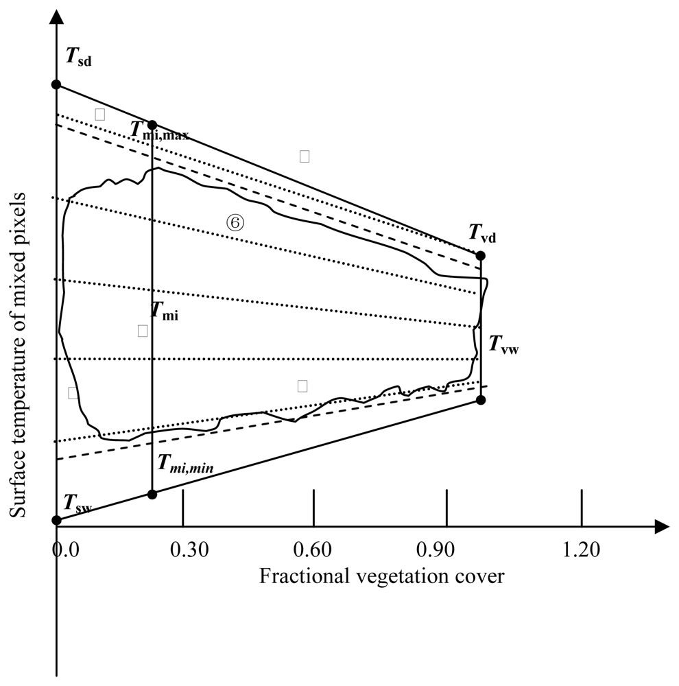
2.1 An interpretation of Tm – f space

Figure 1 provides a conceptual illustration of Tmf space, where “true wet/cool edge” of the trapezoid is related to surface conditions of potential evapotranspiration and has minimum surface resistance to evapotranspiration (rsmin).
Soil water content equals to field capacity; ‘true dry/warm edge’ represents zero evapotranspiration and has maximum surface resistance to evapotranspiration (rsmax). If the positions of the two edges are determined, the shape and the structure of the trapezoid can be fixed and the consequent calculations of the surface heat fluxes could be done. To make the illustration easier to follow, four points are defined: Tsd and Tsw represent the points of true dry bare soil and true water saturated bare soil, respectively. Tvd represents true dry full-cover vegetation and Tvw represents true water saturated, full-cover vegetation. The above definitions all correspond to the ideal surface conditions, namely there exist driest and wettest bare soil and full-cover vegetation. In reality there are always insufficient number of pixels that can cover all kinds of soil wetness and vegetation fraction cover within the study area, which leads to a difficulty in determining “true wet/cool edge” and “true dry/warm edge”, as a result, “observed wet/cool edge” and “observed dry/warm edge” (dashed lines) are often defined according to the envelop shape of the actual scatter plot to represent actual two extreme soil moisture conditions and are used to replace “true wet/cool edge” and “true dry/warm edge” in most applications, although some errors would be introduced. Iso-line of equal vegetation fraction cover intersects “true dry edge” and “true wet edge” at true maximum temperature and true minimum temperature denoted as Tmi,max and Tmi,min, respectively. It has to be noted that for the trapezoid constructed by data with coarser pixel resolution (eg. 1km), surface temperature at “true dry edge” generally is higher than that at “observed dry edge”, contrarily surface temperature at “true wet edge” is lower than that at “observed wet edge” according to the findings of Carlson [9] about the scale issues of trapezoid space. The major reason is the absence of the driest and wettest pixels due to the great mixing effect of the pixel (vegetation/bare soil).

2.2. PCACA Algorithm

The PCACA algorithm is a method to decompose the mixed surface temperature. As mentioned above, its physical basis is the fact that soil water status can be represented by the configuration of Tm-f space, and like the triangle method, the crucial assumption is that surface temperature is mainly controlled by soil water availability [9, 10, 12].
The basic formulations used to decompose mixed surface temperature are shown in Eq. (1) and Eq. (2). The derivations of Eq. (2) can be found in Appendix I.
σ ɛ m T m 4 = σ ɛ veg f T veg 4 + σ ɛ soil ( 1 f ) T soil 4
k = d T m d f T veg T soil
where, εm, εveg and εsoil are the broadband emissivities of mixed pixel, vegetation and bare soil, respectively; σ is the Stefan-Boltzmann constant; dTm/df represents the slope of iso-line of equal soil water availability, expressed as k in the remainder of the paper. In the study, constant εveg of 0.97 and εsoil of 0.95 were used. By simply weighting the fractional cover for vegetation and bare soil, mixed pixel emissivity εm for each pixel can be computed following Eq. (3) [13].
ɛ m = f ɛ veg + ( 1 f ) ɛ soil
From the above three equations, we can see that to solve Tsoil and Tveg, k for each pixel is the key parameter and needs to be obtained firstly.
According to Figure 1, two procedures were needed to derive k in the study: (1) determining the shape of the trapezoid bounded by ‘true dry edge’ and ‘true wet edge’, namely locating the ‘true dry edge’ and ‘true wet edge’ on the trapezoid, and thereby calculating the two slopes of the two bounder lines (ku is for upper bound, kL is for lower bound). A detailed method for this will be illustrated in section 3; (2) linearly interpolating k between the highest and the lowest surface temperature to obtain the slope for each pixel based on the equation below:
k i = T m i T m i , min T m i , max T m i , min ( k u k L ) + k L
Considering that the precise formulation of the relationship is actually unknown, linear interpolation is a reasonable approximation according to the study on the configuration of Tmf space by Calson [9, 10] and Moran [14].

2.3 Layered Energy-separating Algorithm

Essentially, the aim of the Layered Energy-separating algorithm is to calculate Bowen-ratio (β, the radio of sensible heat flux to latent heat flux) of soil and vegetation expressed as βsoil and βveg, respectively. By using the relationship between Water Deficit Index (WDI), evapotranspiration and potential evapotranspiration (λE0) illustrated by Moran et al. [14], Eq. (5) can be derived:
β i T m , max T m , min T m , max T m i 1
where subscript i represents pixel i. From Eq.(5) we can see that β can be obtained conveniently from the data shown on Figure.1.

2.4 Estimation of Other Core Variables

After Ts, Tv, βs and βv are obtained using the above methods, net radiation at the soil surface and at the vegetation surface (Rn,soil, Rn,veg) can be calculated following Eqs. (6) and (7), and thereby soil heat flux and net radiation of mixed pixel can be estimated using the empirical formulation of Eq. (8) and Eq. (9), as used widely in previous studies [15-17].
R n , soil = S 0 ( 1 α soil ) + σ ɛ sky T sky 4 σ ɛ soil T soil 4
R n , veg = S 0 ( 1 α veg ) + σ ɛ sky T sky 4 σ ɛ veg T veg 4
G 0.3 ( 1 0.9 f ) R n , soil
R n = f R n , soil + ( 1 f ) R n , veg
where S0 is the solar incident total radiation and is regarded as spatially uniform for clear sky conditions at the regional scale, usually obtained from standard meteorological station; αsoil and αveg are the albedo of bare soil and vegetation, also calculated by the PCACA algorithm (seen from Appendix И); εsky is the average sky emissivity and is approximately set to 1.0 in the study. Tsky is average sky temperature and usually approximates to the temperature at 37° view sky angle [18], detailed calculation about which will be described in the Section 3.
In terms of the Bowen-ratio energy balance method, soil evaporation (λEsoil) and vegetation transpiration (λEveg) can be retrieved based on Eq. (10). When energy exchange between vegetation and bare soil is neglected, λE of a mixed pixel can be described as a linear combination of λEsoil and λEveg, expressed as Eq. (11).
λ E soil = R n , soil G 1 + β soil , λ E veg = R n , veg 1 + β veg
λ E = f λ E veg + ( 1 f ) λ E soil

3. Two improvements for the two-layer model

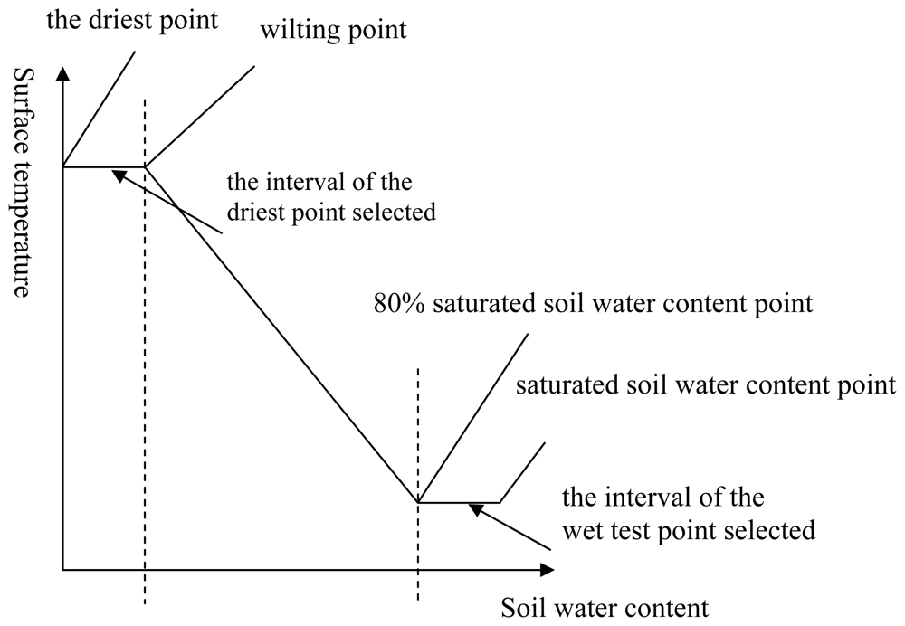
3.1 locating the true dry edge in Tm – f space

As mentioned above, the locations of true dry edge and the true wet edge are crucial in the application of PCACA algorithm. The previously used method to determine the trapezoid boundary often leads to uncertainties because of subjective judgement. To reduce the errors from this respect, a physically based method, which takes account of the surface energy balance, is presented in this study.
According to Figure.1, the four corner points, Tsd, Tsw, Tvd and Tvw can determine the envelop shape of the trapezoid, that is to say, as long as their values are obtained. Consequently, the true dry edge and the true wet edge can be determined. In the study, surface energy balance method was adopted to compute their values. For pixels at the true dry edge, Eq.(12) is used because λE=0. Substituting Rn, G, H for Eq.(9), Eq.(8) and Eq.(13), we obtained Eq.(14) for Tsd. In the same way, Tvd is formulated as Eq.(15).
R n G = H
H = ρ C p ( T s T a ) r a
T s d = 0.7 [ S 0 ( 1 α s d ) + σ ɛ sky T sky 4 ] + ρ C p r sda T sda ρ C p r sda + 0.7 σ ɛ soil T s d 3
T v d = 0.7 [ S 0 ( 1 α v d ) + σ ɛ sky T sky 4 ] + ρ C p r vda T vda ρ C p r vda + 0.7 σ ɛ veg T v d 3
where the subscripts sd, vd represent true driest bare soil and true driest full-cover vegetation, respectively. ρ is density of air, cp is the volumetric heat capacity of air, ra is the air dynamic resistance, σ is the S-B coefficient, αsd is the albedo of dry bare soil.
From these two equations, we can see that Tsd or Tvd could not be iteratively computed until parameters of αsd, αvd, Tsky, rsda, rvda, Tsda, Tvda are acquired. From the Tmf space, the observed driest bare soil and the observed driest full-cover vegetation can be found. Although there are surface temperature differences between them and the true driest bare soil and true driest full-cover vegetation, they represent relative driest and wettest soil conditions. It means that aerodynamic resistance and air temperature of the observed driest bare soil and the observed driest full-cover vegetation are approximate to that of Tsd, Tvd points under the conditions that the variations in atmospheric conditions are very small due to the spatially uniformity. In the study, we chose 50 pixels around the upper-left corner in the trapezoid representing the observed driest bare soil and 50 pixels around upper-right corner in the trapezoid representing the observed driest full-cover vegetation, and the highest Ta and ra in each 50 pixels were selected as Tsda and rsda, Tvda and rvda, respectively. The method of retrieving the spatial distribution of Ta and ra will be described in the following. The calculation of ra requires ea and rs, the retrievals about which will also be described. As for αsd and αvd, we selected the lowest albedo values of bare soil and full-cover vegetation within the whole scene of remotely sensed image (pixels) because low albedo would result in high surface temperature at the same soil water content, judging from Eq. (14) and Eq. (15). The item of σ ɛ sky T sky 4 represents downward long wave radiation that usually has small spatial variability for clear sky, thus can be obtained from the measurements of meteorological stations at the satellite overpass time. The following are the calculations of spatial distributions of Ta, ea, rs and ra:

a) Estimation of air temperature (Ta)

Surface temperature, as a heat or cold source, influences the variations of air temperature by heating or cooling near-surface atmosphere. In most cases, high surface temperature is accompanied by high air temperature and low surface temperature is accompanied by low air temperature. By using this relationship between them and assuming the following ratio expressed in Eq. (16), an interpolation method is presented to map the distribution of air temperature. The numerator and the denominator both represent radiant emission. Because the effects of neighborhood pixels diminish as the distance to the pixel increases, a weight (w) derived from an inverse distance weight (IDW) method is assigned to each neighboring observations, and is given in Eq. (17).
i = 1 n w i σ ɛ a i T a i 4 i = 1 n w i σ ɛ m i T m i 4 = σ ɛ a j T a j 4 σ ɛ m j T m j 4
w i = d i p i = 1 n d i p , ɛ a = 1.24 ( e a T a ) 1 / 7
where i represents the pixel where air temperature measurement is made, j indicates the pixel where no measurements are available and estimate is required; n is the number of air temperature observations; d is the distance between pixel i and pixel j; p is an exponent. The higher the exponent is, the larger the influence of the closest observations on estimate is; p is set to 2 in the study; σ is the Stephen Boltzmann constant; εa is the emissivity of air calculated from Eq. (17) [19].

b) Estimation of actual vapor pressure near surface (ea)

Like the relationship between air temperature and surface temperature, there are also strong interactions between near-surface actual vapor pressure and soil moisture. If there is no horizontal and vertical advection, vapor in the atmosphere mainly comes from soil water by an evapotranspiration process. Contrarily, the vapor gradient between surface and air influences the intensity of evapotranspiration. By assuming the following ratio relationship between near-surface actual vapor pressure and soil water, we interpolated ea, where soil moisture status was characterized quantitatively by the soil apparent thermal inertia:
R n 2 ( T s T min ) Δ t 1 2 i = 1 n w i e a i i = 1 n w i R n i ( T m i T min ) = e a j R n j ( T m j T min )
where i, j, wi, Ts have the same meanings as in Eqs. (16) and (17); Tmin is the minimum surface temperature during the daytime which usually occurs before sunrise when Rn=0 and for all pixels it can be assumed to be the same value [20]. Δt is the time interval between sunrise and the satellite overpass time.

c) Estimation of surface resistance to evapotranspiration (rs)

In the retrieval of evapotranspiration, rs is used to correct the difference between the vapor pressure at the surface (es) and the saturated vapor pressure at the evaporating front (es*). In theory, rs ranges from ∞ to 0 corresponding to the surface conditions of potential evapotranspiration and zero evapotranspiration, respectively, namely the true dry edge and the true wet edge. However, in reality the condition of zero evapotranspiration (rsmax = ∞) rarely occurs for vegetated surface even in semi-arid environment primary due to root zone soil water uptake, consequently, we selected a pixel closest to the observed driest bare soil where a meteorological station is located to calculate rsmax by λE, ea, u measurements at the satellite overpass time. rsmax is about 1000 (s m-1) according to the calculation, which is in agreement with Qiu's observations [21]; rsmin is set to 0 in the study.
After the upper and lower limits of rs are determined, rs is interpolated linearly within each f interval between the lowest and the highest temperature. Following the illustrations in Figure 1, rsi for a pixel at (fi , Ti) equals:
r s i = T s i T s i , min T s i , max T s i , min ( r s max r s min ) + r s min
The interpretation is similar to the method used by Stisen et al. [11]. The difference is that Stisen et al. used Priestly-Taylor parameter to represent an effective surface resistance to evapotranspiration.

d) Estimation of aerodynamic resistance (ra)

Besides air temperature, aerodynamic resistance is a site-specific variable and can not be retrieved directly by remote sensing. Although Monin-Obukhov similarity theory has been widely used to estimate it, the accurate calculations for the spatial distributions of roughness length (Z0), wind speed (u) and the atmospheric stability parameters are very difficult. In this study, we adopted the energy balance method.
An expression of ra is obtained on the basis of the energy-balance by substituting Rn, G, H and λE for Eq. (9), Eq. (8), Eq. (13) and Eq. (20):
λ E = ρ c p ( e s * e a ) γ ( r s + r a )
a 1 r a 2 + a 2 r a + a 3 = 0 a 1 = ( 0.7 + 0.27 f ) γ R n a 2 = ( 0.7 + 0.27 f ) γ R n r s ρ c p γ ( T m T a ) ρ c p ( e s * e a ) a 3 = ρ c p γ ( T m T a ) r s
where γ is the psychometric constant, es* is the saturated vapor pressure at Tm estimated using the classic formulation with regard to surface temperature, as Eq. (22), other parameters have the same meanings as the above illustrations. Here, Ta, ea and rs are estimated by the approaches mentioned previously.
e s * = 6.1078 exp ( 17.27 T m T m + 237.3 )
Above all, all necessary parameters to calculate Tsd, Tvd can be retrieved according to the Eqs. (12)(22) in combination with limited ancillary data. Here, Tm and αm is obtained from MODIS (Moderate Resolution Imaging Spectroradiometer) standard land data products, MOD11 and MOD02 [22, 23], through the NASA Earth Observing System Data Gateway.

3.2 Locating the true wet edge in Tm – f space

Many studies [9, 24, 25] indicated that the dry edge is more evident than the wet edge in the Tmf space. There often exist outlying points exhibiting a tail toward low values of temperature and f. Such points may represent anomalous surfaces mainly due to cloud contamination and usually are discarded from the analysis [10]. Thus, although Tsw and Tvw also can be parameterized on the basis of energy balance equation like Tsd and Tvd, the inputs (αsd, αvd, rsda, rvda, Tsda, Tvda) cannot be obtained by the above methods. Taking account of the fact that the surface radiant temperature of dense vegetation is very close to the ambient air temperature [9, 26, 27], we took the average air temperature at f =1 as Tvw. As for Tsw, we adopted an approximation of using the surface temperature of standing water body (such lake) as the surface temperature of true wet bare soil Tsw, that is to say, standing water body is regarded as the surface of potential evapotranspiration. In fact, it is not uncommon to find some patches of standing water body in a remote sensed image. In this study, the surface temperature of Dongping Lake (35.965°, 116.81°; water area: 209 km2) was used as Tsw. In applications, we found that the pixels with mixed surface temperatures below the true wet edge all scattered around the cloud pixels and the coastline pixels.

3.3 Physical illustrations for the uncertainties using the above locating methods

Using the above methods, the positions of the true dry edge and the true wet edge in the triangle can be located. When surface radiant temperature is mainly dominated by surface soil water content, the following relationship between surface temperature and soil water content is tenable (Figure 2), which has been illustrated in the Qiu's experiment [21]. Figure 2 suggests that when the soil water content ranges from 80% to 100% of the soil saturation, evapotranspiration will happen approximately at the level of potential Evapotranspiration. On the contrary, when the range of the soil water content is from the wilting point to the driest, evapotranspiration is close to zero, and in the two extreme conditions, surface temperature can be regarded as a constant due to the same evaporative cooling effect. On the basis of this, although the true driest and the true wettest points can't be determined using the above methods, the errors will be acceptable in the determination of Tsd, Tsw, Tvd and Tvw due to the constant surface temperature.

3.4 Elimination of the effects of atmospheric conditions on surface evapotranspiration

Same as the triangle method, an important assumption for the PCACA algorithm is that the surface evapotranspiration is primarily constrained by soil water availability, based on which Tsoil values for all pixels with an equal water availability are identical, so are for Tveg values, that is to say, the configuration of Ts and f is mainly caused by the variation of the soil water availability and is irrelevant to the differences in atmospheric conditions and surface properties [11]. However, in reality it is not true that the atmospheric conditions and surface properties are entirely homogeneous within the large study area. There exist some differences eg. in wind speed, air temperature, surface roughness length and surface albedo, which are all site-specific variables. As a result, it will lead to the the variability of the surface evapotranspiration and thereby influence the surface temperature and the configuration of Ts and f. To satisfy the assumption, the effects of these factors need to be eliminated.
In the study, the effects of four controlling factors (ra, ea, Ta and albedo) on surface temperature were eliminated. According to the assumption, ra, ea, Ta and albedo values of each pixel should be equal, namely they are spatially homogeneous, to ensure that only water availability controls surface temperature. To meet this requirement, the average values of ra, ea, Ta and albedo in the image are assigned to each pixel and a new mixed surface temperature (Tmi’ ) is calculated based on energy balance equation. Tmi’ is the assumed temperature controlled only by soil water availability and therefore the new trapezoid constructed by Tm and f is more meaningful for the PCACA algorithm. It has to be noted that although the configuration of Tm’ – f space is different from that of the Tmf space, the locations of the true dry edge and the true wet edge in the trapezoid don't change since the two theoretical extreme soil water status at the satellite overpass time are the same. On the basis of Tm’, Tveg’ (vegetation temperature controlled only by soil water availability) and Tsoil’ (soil temperature controlled only by soil water availability) can be obtained. Now the problem is that the calculated Tveg’ and Tsoil’ cannot represent the actual temperature of vegetation and soil after the above transformation., Therefore they can't be directly used in the consequent calculations. To estimate the true vegetation temperature and true soil temperature (Tveg and Tsoil) from Tveg’ and Tsoil’, the following method is used.
Assuming that the thermal energy fraction assigned to the vegetation and the soil are constants, the following expression [Eq. (23)] can be approximated. The left item represents the proportion of thermal energy difference for vegetation or soil to the total thermal energy difference, and the right item represents the proportion of vegetative or soil thermal energy to the total thermal energy. It suggests that changes of environmental conditions bring same effects on vegetation temperature, soil temperature and mixed surface temperature, for example, Tsoil, Tveg and Tm values would all increase with the increase of solar radiation intensity and all influenced by wind speed. It is not likely to happen that the Tsoil increases, but Tveg decreases in the same atmospheric conditions. Therefore, the assumption is reasonable in practice and it is different from Beer's law using fractional vegetation cover as the weight to partition thermal energy. Using this equation, Tsoil4 - Tveg4 can be solved as Eq. (24).
T veg 4 T veg 4 T m 4 T m 4 T veg 4 T m 4 , T soil 4 T soil 4 T m 4 T m 4 T soil 4 T m 4
T veg 4 T soil 4 = T m 4 T m 4 ( T veg 4 T soil 4 )
Combined with Eqs. (1) and (24), Tsoil and Tveg can be solved. Tsoil and Tveg can be directly obtained from Eq. (23), at the same time the uncertainties of the solution can be reduced to the minimum by this method because the difference between Tsoil and Tveg is used instead of the absolute temperatures and Eq.(1) helps to maintain the thermal energy balance in the calculation of Tsoil and Tveg values.

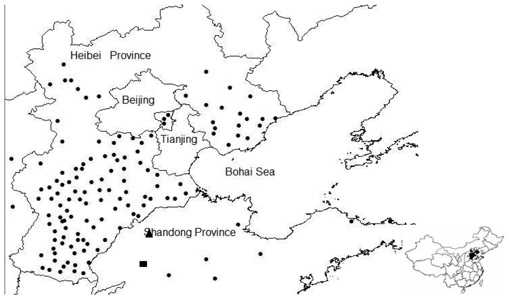
4. Study area and field measurements

The study area is located in the North China Plain and ranges from 35.2N to 40.84N in latitude, from 113.68E to 119.54E in longitude. The land use in the area is dominated by the rotating cropping of winter wheat and summer maize. Millet, soybean and cotton are also scattered planted in summer [28]. According to the traditional tillage practice, winter wheat is sown in early October, harvested in early or mid June next year, and summer maize is planted in early to mid June and harvested at the end of September. The soil is mostly silt, light loam and medium loam. Annual precipitation is about 600 mm, more than 50% of which falls during the summer monsoon between July and September. The groundwater table varies from 1.5 m to 3.5 m with an average of 2.5 m.
In the study, field measurements from 135 standard meteorological stations were used. The measurements include air temperature and actual vapor pressure at 2 m height above the surface, solar incoming radiation, surface radiative temperature, wind speed, upward longwave radiation, upward shortwave radiation, downward longwave radiation and downward shortwave radiation. Figure.3 shows the spatial distribution of these stations in the study area, where the triangle symbol (▲) marks the location of Yucheng Agro-ecosystem Station that can represents the largest agricultural area in the North China Plain [29]. Sensible heat flux and latent heat flux have been continuously measured by the Eddy Correlation (EC) system which is composed of a 3D sonic anemometer and an open path CO2/H2O analyzer since 2002. H, λE and CO2 fluxes were originally sampled at 10 Hz and values averaged over 30 min were used in the study to validate the above mentioned methods. The rectangle symbol (■) shows the location of Dongping Lake. Water surface temperature has been measured for seven years since 2001 and was used to validate the MODIS land surface temperature products used in this study, and thereby to ensure the accuracy of Tsw values.

5. Satellite data

MODIS land data products, including MOD11 (Land Surface Temperature), MOD03 (Geolocation Data Set), MOD05 (Total Precipitable Water), MOD02 (Calibrated Geolocated Radiance) and MOD35 (Cloud Mask), for clear sky during springtime between Mar and June when winter wheat is the dominant crop were used in the study. The visible channels of MOD02 were processed with atmospheric correction using the SMAC algorithm [30] with the combination of the MOD03 and MOD05 data. The cloud was masked out based on MOD35 data. The basic variables used as inputs in the model consist of albedo, fractional vegetation cover and surface temperature, based on which the calculation of Rn, PCACA algorithm and Layered Energy-separating Algorithm were applied.
The instantaneous surface albedo was obtained by averaging reflectance values for several visible and near-infrared channels with the wavelength as the weight. This would introduce some errors because channel reflectance values observed by a satellite are reflectance at only one Sun-target-sensor configurations and it is generally different from the hemispherical reflectance. But we assumed its influence to be small as pointed by Nishida [27]. The fractional vegetation cover was estimated from the normalized difference vegetation index (NDVI) [27], as Eq.(25).
f = NDVI NDVI min NDVI max NDVI min
where NDVImax and NDVImin are NDVI values for full cover vegetation (f=1) and bare soil (f=0). According to the field NDVI measurements performed at Yucheng station, NDVImin=0.09 and NDVImax=0.78. Other variables, such as Rn, G, Ta, ea, rs, were obtained using the above mentioned methods.

6. Results and Discussion

Figure 4 shows the comparisons between Tsoil, Tveg obtained from the original model and Tsoil’, Tveg’ obtained from the improved model at an iso-line of equal water availability.
Apparently, the results of Tsoil’, Tveg’ are in closer agreement with the above assumptions that soil surface temperature for all pixels at an iso-line are identical, so are the vegetative surface temperature. It provides a better physical foundation for the model.
Due to the absence separate measurement of the soil evaporation, soil heat flux, vegetation transpiration and vegetation heat flux from the field sit, estimates of Rn-G and λE from the model were compared to the measurements from Yucheng station, as shown in Figure 5 for available energy (Rn-G), in Figure 6 for λE.
Because direct comparison of λEsoil and λEveg cannot be performed, the relationship between modeled λEveg and measured CO2 were used to indirectly validate the two-layer model since CO2 fluxes are closely related to λEveg[31, 32]. Figure 7 shows the scatter plot between modeled λEveg and measured CO2 flux. Note that the minus sign (-) for CO2 fluxes means that the flux transferring direction is from up to down. The performance of the model was evaluated using the root mean squares difference (RMSD) and the mean absolute difference (MAD), which are defined as Eq.(26) and Eq.(27), respectively.
RMSD = [ i = 1 n ( P i O i ) 2 / n ] 1 / 2
MAD = i = 1 n | P i O i | / n ]
where n is the number of observations, P represents the model estimated value, O represents the observed value.
The figures demonstrate that (1) no significant bias is found between the modeled and measured Rn-G with RMSD=46.3 and MAD=40.2. The high correlation coefficient (r2=0.79) suggests that Rn, soil and Rn, veg calculated from Tsoil and Tveg are reasonable because Rn is calculated by them; (2) estimates of λE tends to overestimate for lower λE values and shows larger bias than Rn-G resulting in 54.1 of RMSD and 47.7 of MAD, which implies a larger uncertainty of the model in low λE conditions; (3) in general, seasonal variations in modeled λEveg and measured CO2 flux shows good agreement though few points in 2006 showed different variations perhaps influenced by horizontal/vertical advection or other factors. Vegetation transpiration generally increases with the crop growth, at the same time, since vegetation absorbs more CO2 due to the more active photosynthesis in the daytime, CO2 fluxes also increases. On the contrary, λEveg and CO2 fluxes both became very small after crop harvest or in winter. In the study, winter wheat was harvest in June, therefore λEveg and CO2 fluxes rapidly decreased on June 15 and June 19 in 2005. Figure 7 indirectly proves the soundness of the two-layer model to estimate the soil evaporation and vegetation transpiration separately.
In fact, there are two other factors which contribute to the uncertainty in the above validation. One is that point measurements usually can not represent the whole MODIS pixel (1 km2) because of the large scale disparity between them. The other is that the observed Rn, λE, H and G values at field cannot meet the surface energy balance closure resulting from many possibilities, such as instrumental errors, horizontal/vertical advections [33-35], however, the basis of the model used in the study is the surface energy balance, as most remote sensing models of evapotranspiration, such as SEBS [36], SEBAL [37], N95 [3]. Therefore, it is not uncommon to see the differences between modeled fluxes and observed ones. Compared with other studies, the RMSD of 54.1 (w/m2) for modeledλE are in a acceptable range [17, 27, 38, 39].
Figure 8 shows the λEveg maps on May 2, 2005 for the North China Plain retrieved by the improved model and the original model, respectively. Differences were found between them. The λEveg value from the improved model varies from 222 (w/m2) to 456 (w/m2), while the original λEveg values varied from 50 (w/m2) to 560 (w/m2). In terms of the experiences and the knowledge on the vegetation transpiration, a small λEveg dynamical range is more reasonable in the rapid growing season of winter wheat, that is to say, the results from the improved model is better than that of the original model although it is difficult to quantitatively evaluate the two results due to the absence of field measurements of the vegetation transpiration and soil evaporation at the satellite pixel scale. Furthermore, according to the above illustrations, the physical basis of the improved model is strengthened against the original model.

7. Conclusions

This paper presented two improvements of a two-layer model for the estimation of the land surface heat fluxes. The weakness in the original model was identified: (1) a subjective method to determine the true boundary lines from the scatter plot for the surface temperature of mixed pixel versus the fractional vegetation cover; (2) the assumption that the configuration of Tmf space is mainly controlled by soil water availability, are not physically realistic. To investigate the two issues and obtain more realistic separation of the surface temperature for the soil and vegetation components, and thereby more accurate partitioning of the surface fluxes for the soil and vegetation components, introducing the surface energy balance method solves the problem (1) and the method of eliminating the effects of four controlling factors (ra, ea, Ta and albedo) on surface temperature solves the problem (2). At the same time, the interpolation methods of Ta and ea, the methods for acquiring spatial distributions of ra and rs were also investigated. Finally, the improved model was applied to the North China Plain. The results showed good agreement with in situ terrestrial surface fluxes measurements. Furthermore, by comparing the seasonal variations of vegetation transpiration and CO2 flux, and the vegetation transpirations retrieved by the improved model and the original model, the effectiveness of the improved two-layer model for estimating soil evaporation and vegetation transpiration were indirectly proved.

Acknowledgments

This work was supported jointly by the State Key Development Program for Basic Research of China with grant number 2007CB714401-3, the Knowledge Innovation Project of IGSNRR, CAS (grant No. GXIOG-A05-11), the Knowledge Innovation Program of CAS (grant No. KZCX2-YW-326), the Young Talents Forefront Project of IGSNRR, CAS (grant No.07v70050SZ), the National Key Project of Scientific and Technical Supporting Programs Funded by Ministry of Science & Technology of China (No. 2006BAC08B0407) and the Program of “One Hundred Talented People” of the Chinese Academy of Sciences (CAS)

Appendix I

The relationship between the temperature of mixed pixel and vegetative fractional cover for 8∼14μm can be expressed as:
σ ɛ m T m 4 = σ ɛ veg f T veg 4 + σ ɛ soil ( 1 f ) T soil 4
where Tm, Tveg and Tsoil are respectively the surface temperature of mixed pixel, vegetation canopy and soil surface. εm, εveg and εsoil are the emissivities of mixed pixel, vegetation and bare soil; σ is the Stefan-Boltzmann constant. f is fractional vegetation cover of mixed pixel. Evidently, Tveg and Tsoil cannot be retrieved only using this equation. Computing the differential coefficient of Tm to f and assuming
d T veg d f 0 , d T soil d f 0 ,
we can get Eq. (AI.2):
4 ɛ m T m 3 = d T m d f + T m 4 d ɛ m d f = ɛ veg T veg 4 ɛ soil T soil 4
Multiplying f in the two sides of Eq (AI.2) and rearranging this equation, we obtained:
f ( 4 ɛ m T m 3 = d T m d f + T m 4 d ɛ m d f ) = f ɛ veg T veg 4 f ɛ soil T soil 4
Integrating Eq. (AI.2) with Eq. (AI.3), Tsoil can be expressed as:
T soil = { 1 ɛ soil [ ɛ m T m 4 f ( T m 4 d ɛ m d f + 4 ɛ m T m 3 d T m d f ) ] } 1 / 4
in the same way, Tveg can be expressed as:
T veg = { 1 ɛ veg [ ɛ m T m 4 + ( 1 f ) ( T m 4 d ɛ m d f + 4 ɛ m T m 3 d T m d f ) ] } 1 / 4
According to Eq. (3), d ɛ m d f = ɛ veg ɛ soil. In the study, d ɛ m d f = 0.02 due to the fixed values of εveg=0.97 and εsoil=0.95. In terms of the numerical simulations, the small d ɛ m d f value has small influence on the difference between Tsoil and Tveg, therefore we ignored the difference between εveg and εsoil. This simplification means that Eq. (AI.1) was simplified as Eq. (AI.6), which is also reasonable in applications [5].
T m 4 = f T veg 4 + ( 1 f ) T soil 4
Furthermore, using Eq.(AI.5) minus Eq.(AI.4), the following expression can be simplified as:
T veg 4 T soil 4 4 T m 3 d T m d f
In fact, T veg 4 T soil 4 4 ( T veg T soil ) T m 3 when no large temperature difference between vegetation surface and soil surface occurs, so d T m d f can be formulated as:
d T m d f T veg T soil

Appendix И

Albedo of mixed pixel is the weighed-average value of soil albedo and vegetation albedo, showed as Eq. (AИ.1). Computing the differential coefficient of αm to f and assuming d α veg d f 0, d α soil d f 0, we obtained Eq.(AИ.2).
α m = α soil + f α veg ( A H . 1 )
d α m d f α veg α soil
Integrating Eq. (AИ.1) with Eq. (AИ.2), αsoil and αveg can be expressed as:
α soil = α m f d α m d f
α veg = α m + ( 1 f ) d α m d f
Evidently, as the method of decomposing mixed surface temperature Tm, PCACA also can be applied to separate albedo of mixed pixel using the configuration of αm- f space.

References and Notes

  1. Su, H.B.; McCabe, M.F.; Wood, E.F.; Su, Z.; Prueger, J.H. Modeling evapotranspiration during SMACEX: Comparing two approaches for local- and regional-scale prediction. J. Hydrometeorol. 2005, 6, 910–922. [Google Scholar]
  2. Verhoef, A.; De Bruin, H.A.R.; Van den Hurk, B.J.I.M. Some practical notes on the parameter kB-1 for sparse vegetation. J. Appl. Meteor. 1997, 36, 560–572. [Google Scholar]
  3. Norman, J.M.; Kustas, W.P.; Humes, K.S. A two-source approach for estimating soil and vegetation energy fluxes from observation of directional radiometric surface temperature. Agric. For. Meteorol. 1995, 77, 263–293. [Google Scholar]
  4. Kustas, W.P.; Norman, J.M. Evaluation of soil and vegetation heat flux predictions using a simple two-source model with radiometric temperatures for partial canopy cover. Agric. For. Meteorol. 1999, 94, 13–29. [Google Scholar]
  5. Kustas, W.P.; Norman, J.M. Evaluating the Effects of Subpixel Heterogeneity on Pixel Average Fluxes. Remote Sens. Environ. 2000, 74, 327–342. [Google Scholar]
  6. Zhang, R.H.; Sun, X.M.; Wang, W.M.; Xu, J.J.; Zhu, Z.L.; Tian, J. An operational two-layer remote sensing model to estimate surface flux in regional scale: physical background. Sci in China Ser. D. 2005, 48, 225–244. [Google Scholar]
  7. Gillies, R.R.; Carlson, T.N.; Cui, J.; Kustas, W.P.; Humes, K.S. A verification of the ‘triangle’ method for obtaining surface soil water content and energy fluxes from remote measurements of the Normalized Difference Vegetation Index (NDVI) and surface radiant temperature. Int. J. Remote Sens. 1997, 18, 3145–3166. [Google Scholar]
  8. Sandholt, I.; Rasmussen, K.; Andersen, J. A simple interpretation of the surface temperature / vegetation index space for assessment of surface moisture status. Remote Sens. Environ. 2002, 79, 13–224. [Google Scholar]
  9. Carlson, T.N.; Gillies, R.R.; Schmugge, T.J. An Interpretation of Methodologies for Indirect Measurement of Soil-Water Content. Agric. For. Meteorol. 1995, 77, 191–205. [Google Scholar]
  10. Carlson, Toby. An Overview of the “Triangle Method” for Estimating Surface Evapotranspiration and Soil Moisture from Satellite Imagery. Sens. 2007, 7, 1612–1629. [Google Scholar]
  11. Stisen, S.; Sandholt, I.; Norgaard, A.; Fensholt, R.; Jensen. Combining the triangle method with thermal inertia to estimate regional evapotranspiration – Applied to MSG-SEVIRI data in the Senegal River basin. Remote Sens. Environ. 2008, 112, 1242–1255. [Google Scholar]
  12. Carlson, T.N.; Gillies, R.R.; Perry, E.M. A Method to Make Use of Thermal Infrared Temperature and NDVI measurements to Infer Surface Soil Water Content and Fractional Vegetation Cover. Remote Sens. Rev. 1994, 9, 161–173. [Google Scholar]
  13. Valor, E.; Caselles, V. Mapping Land Surface Emissivity from NDVI: Application to European, African, and South American Areas. Remote Sens. Environ. 1996, 57, 167–184. [Google Scholar]
  14. Moran, M.S.; Clarke, T.R.; Inoue, Y.; Vidal, A. Estimating crop water deficit using the relation between surface-air temperature and spectral vegetation index. Remote Sens. Environ. 1994, 49, 246–263. [Google Scholar]
  15. Santanello, J.A.; Friedl, M.A. Diurnal covariation in soil heat flux and net radiation. J. Appl. Meteor. 2003, 42, 851–862. [Google Scholar]
  16. Kustas, W.P.; Li, F.; Jackson, T.J.; Prueger, J.H.; MacPherson, J.I.; Wolde, M. Effects of remote sensing pixel resolution on modeled energy flux variability of croplands in Iowa. Remote Sens. Environ. 2004, 92, 535–547. [Google Scholar]
  17. Batra, N.; Islam, S.; Venturini, V.; Bisht, G.; Jiang, J. Estimation and comparison of evapotranspiration from MODIS and AVHRR sensors for clear sky days over the Southern Great Plains. Remote Sens. Environ. 2006, 103, 1–15. [Google Scholar]
  18. Zhang, R. Experimental Remote Sensing Modeling and Surface Foundations; Sciences Press: Beijing, 1996. [Google Scholar]
  19. On a derivable formula for long-wave radiation from clear skies. Water Resour. Res. 1975, 11, 742–744.
  20. Zhang, R.H.; Sun, X.M.; Zhu, Z.L.; Su, H.B.; Tang, X.Z. A remote sensing model for monitoring soil evaporation based on differential thermal inertia and its validation. Sci. China Ser. D. 2003, 46, 344–355. [Google Scholar]
  21. Qiu, G.Y.; Shi, P.J.; Wang, L.M. Theoretical analysis of a remotely measurable soil evaporation transfer coefficient. Remote Sens. Environ. 2006, 101, 390–398. [Google Scholar]
  22. Wan, Z.; Zhang, Y.; Zhang, Q.; Li, Z.-L. Quality assessment and validation of the MODIS global land surface temperature. Int. J. Remote Sens. 2004, 261–274. [Google Scholar]
  23. Justice, C.O.; Vermote, E.; Townshend, J.G.R.; Defries, R.; Roy, D.P.; Hall, D.K.; Salomonson, V.V.; Privette, J.L.; Riggs, G.; Strahler, A.; Lucht, W.; Myneni, R.B.; Yuri Knyazikhin, Y.; Running, S.W.; Nemani, R.R.; Wan, Z.; Huete, A.R.; van Leeuwen, W.; Wolfe, R.E.; Giglio, L.; Muller, J.P.; Lewis, P.; Barnsley, M.J. The Moderate Resolution Imaging Spectroradiometer (MODIS): land remote sensing for global change research. IEEE Trans. Geosci. Remote Sens. 1998, 36, 1228–1249. [Google Scholar]
  24. Carlson, T.N.; Ripley, D.A.J. On the Relationship Between NDVI, Fractional Vegetation Cover and Leaf Area Index. Remote Sens. Environ. 1997, 62, 241–252. [Google Scholar]
  25. Jiang, L.; Islam, S.; Carlson, T.N. Uncertainties in latent heat flux measurement and estimation: implications for using a simplified approach with remote sensing data. Can. J. Remote Sens. 2004, 30, 769–787. [Google Scholar]
  26. Prihodko, L.; Goward, S.N. Esitmation of air temperature from remotely sensed surface observations. Remote Sens. Environ. 1997, 60, 335–346. [Google Scholar]
  27. Nishida, K.; Namani, R.R.; Running, S.W.; Glassy, J.M. An operational remote sensing algorithm of land surface evaporation. J. Geophys. Res. 2003, 108(D9), 42–70. [Google Scholar]
  28. Mo, X.; Liu, S.; Lin, Z.; Xu, Y.; McVicar, T.R. Prediction of crop yield, water consumption and water use efficiency with a SVAT-crop growth model using remotely sensed data on the North China Plain. Eco. Modelling 2005, 183, 301–322. [Google Scholar]
  29. Zhao, F.H.; Yu, G.R.; Li, S.G.; Ren, C.Y.; Sun, X.M.; Mi, N.; Li, J.; Zhu, Ouyang. Canopy water use efficiency of winter wheat in the North China Plain. Agric. Water. Manage. 2007, 93, 99–108. [Google Scholar]
  30. Rahman, H.; Dedieu, G. SMAC: a simplified method for the atmospheric correction of satellite measurements in the solar spectrum. Int. J. Remote Sens. 1994, 15, 123–143. [Google Scholar]
  31. Zhang, R.H.; Sun, X.M.; Zhu, Z.L.; Su, H.B.; Chen, G. A remote sensing model of CO2 flux for wheat and studying of regional distribution. Sci. in China Ser. D. 1999, 42, 325–336. [Google Scholar]
  32. Wang, S.S. Simulation of Evapotranspiration and Its Response to Plant Water and CO2 Transfer Dynamics. J. Hydrometeorol. 2008, 9, 426–443. [Google Scholar]
  33. Tilden, P.M.; Steven, E. H. An assessment of storage terms in the surface energy balance of maize and soybean. Agric. For. Meteorol. 2004, 125, 105–115. [Google Scholar]
  34. Tian, J.; Zhang, R.H.; Sun, X.M.; Zhu, Z.L.; Zhou, Y.L. Study of a model for correcting the effects of horizontal advection on surface fluxes measurement based on remote sensing. Sci in China Ser. D. 2006, 49, 273–280. [Google Scholar]
  35. Wilson, K.; Goldstein, A.; Falge, E.; Aubinet, M.; Baldocchi, D.; Berbigier, P.; Bernhofer, Ch.; Ceulemans, R.; Dolman, H.; Field, C.; Grelle, A.; Law, B.; Meyers, T.; Moncrieff, J.; Monson, R.; Oechel, W.; Tenhunen, J.; Valentini, R.; Verma, S. Energy balance closure at FLUXNET sites. Agric. For. Meteorol. 2002, 113, 223–243. [Google Scholar]
  36. Su, Z.-B. The surface energy balance system (SEBS) for estimation of turbulent heat fluxes. Hydrol. Earth Syst. Sci. 2002, 6, 85–89. [Google Scholar]
  37. Bastiaanssen, W.G.M.; Menenti, M.; Feddes, R.A.; Holtslag, A.A.M. A remote sensing surface energy balance algorithm for land(SEBAL) 1. Formulation. J. Hydro. 1998, 212, 198–212. [Google Scholar]
  38. Jiang, L.; Islam, S. An intercomparison of regional latent heat flux estimation using remote sensing data. Int. J. Remote Sens. 2003, 24, 2221–2236. [Google Scholar]
  39. Wang, K.C.; Li, Z.Q.; Cribb, M. Estimation of evaporative fraction from a combination of day and night land surface temperatures and NDVI: a new method to determine the Priestley–Taylor parameter. Remote Sens. Environ. 2006, 102, 293–305. [Google Scholar]
Figure 1. Scatter plot of surface temperature against vegetation fraction cover □ true dry edge □ observed dry edge □ observed wet edge □ true wet edge □ iso-line of equal vegetation fraction cover □ iso-line of equal soil water availability.
Sensors 08 06165f1
Figure 2. Relationship between surface temperature and soil water content.
Sensors 08 06165f2
Figure 3. Spatial distribution of standard meteorological stations in the study area.
Sensors 08 06165f3
Figure 4. Comparisons between Tsoil, Tveg obtained from the original model and Tsoil’, Tveg’ obtained from the improved model at iso-line of equal water availability.
Sensors 08 06165f4
Figure 5. Modeled versus measured available energy, Rn-G. The line represents a 1: 1 relationship.
Sensors 08 06165f5
Figure 6. Modeled versus measured latent heat flux, λE. The line represents a 1: 1 relationship.
Sensors 08 06165f6
Figure 7. Seasonal variation of the modeled λEveg and measured CO2 flux during winter wheat growing period 2005 and 2006 (from March to June).
Sensors 08 06165f7
Figure 8. λEveg maps on May 2, 2005 in North China Plain retrieved by the improved model (left image) and the original model (right image).
Sensors 08 06165f8

