1. Introduction
Remotely detecting and identifying weak gaseous plumes using infrared measurement instruments is a challenge that receives continual attention. Burr and Hengartner [
1] have provided a comprehensive review of this problem. Generally, the ability to detect a gaseous effluent is influenced by its concentration pathlength, atmospheric interferences, the temperature difference between the plume and the background surface, the emissivity of the background, and the complexity of the background surface. Collectively, these elements are termed clutter.
When trying to detect and identify gaseous effluents, the type and variability of background clutter in an image presents many modeling challenges. This subject is complex and has been studied from many perspectives. There have been several studies that address the characterization of background clutter [
2,
3]. Endmember estimation is another method that models the types of clutter in an image on a subpixel (multiple background types within a pixel) level [
4,
5]. There are also several studies that address signal-to-noise (SNR) and signal-to-clutter (SCR) ratios [
6,
7]. These terms are used to represent the performance of least squares approaches to gas detection.
This paper studies the background clutter from a different perspective. We explore the effect of the background emissivity on the chemical signal as influenced by the temperature emissivity (
TE) contrast; that is, we identify when the background emissivity will have inhibiting effects on the signal strength and in turn reduce SCR. We view the temperature emissivity contrast as a difference in radiance signal contribution of the plume and the background. First, we isolate the
TE in a formulation of the physics-based radiance model. Then, we conduct analyses of the
TE's contribution to the chemical signal while isolating the effect of the background emissivity. We describe the contributions of these terms to the chemical signal and identify cases where the plume/ground temperatures and background emissivity have amplifying/inhibiting contributions to the signal. To illustrate our claims, we simulate and analyze simplified hyperspectral images using the InfraRed Systems Analysis in General Environments (IR-SAGE) code [
8–
10].
This paper is organized as follows. Section 2 states the physics-based radiance model along with the analyses of the temperature emissivity contrast. Section 3 describes image simulation and gas detection methods. Section 4 presents results of the simulation studies. Section 5 presents conclusions.
2. Physics-Based Radiance Model and Analysis
We explore the three-layer physics-based radiance model to gain insight into how the structure of the background emissivity impacts the at-sensor observed plume signal [
1,
11,
12]. This model can be written as
where
Lobs (
ν) represents sensor-recorded radiance in
W/
cm2*
Sr*
cm−1 at wavenumber
ν (
cm−1),
τa(
ν) and
τp(
ν) are dimensionless terms representing the atmosphere and plume transmissivity, respectively,
B(
T; ν) has radiance units and is Planck's Blackbody function at wavenumber
ν and temperature
T (K),
Lg(
ν) and
Lu(
ν) are the ground-leaving and atmospheric upwelling radiances, respectively, and
e(
ν) includes unmodeled effects and sensor noise [
2,
3].
Following the convention of [
1,
13], we model the ground-leaving radiance as
where
ϵg(
ν) is a dimensionless quantity representing the emissivity of the ground at wavenumber
ν, and 0 ≤
ϵg(
ν) ≤ 1. Note that this formulation ignores the reflected atmospheric downwelling radiance. This assumption is reasonable in the Longwave Infrared band (LWIR) because the reflected radiance contribution to observed signal is negligible [
13].
The Beer-Bourger-Lambert Law [
14] gives an explicit expression for the transmissivity of a gas in terms of the chemical effluent's concentration path-length,
c (with
c measured in parts-per-million-meter, denote
dppm-m), as follows:
where
A(
ν) is the absorbance coefficient of the gas in
ppm-m−1 [
14]. For optically thin plumes, this term is well approximated by the first two terms in a Taylor Series expansion [
1]. This gives
for small
c.
We now substitute
Eq. (2) and
Eq. (4) into
Eq. (1) to arrive at the working-gas-plume linear model
which we interrogate further.
The right hand side of
Eq. (5) shows that atmospheric radiance observed by the sensor is an additive layering of upwelling radiance
Lu(
ν), ground radiance attenuated by atmosphere
τa(
ν)
Lg(
ν), and the signal due to the chemical plume
τa(
ν) [
B(
Tp;
ν) −
ϵg(
ν)
B(
Tg;
ν)]
A(
ν)
c. This representation has been used to motivate scene whitening and the use of least squares approaches for gas detection [
1,
12]. We will use this formulation to explore the effect that background emissivity and the ground/plume temperatures have on the chemical signal.
The radiance due to the chemical plume is the first term on the right hand side of
Eq. (5), namely
We will refer to Expression (6) as the
chemical signal throughout the remainder of the paper. Inspection of this term shows that radiance due to the plume is a function of atmospheric transmission, plume and ground temperature, ground emissivity, and the plume gas absorbance and concentration path length. We note that while Expression (6) is one possible formulation for the chemical signal, there may be other approaches; for example, alternate formulations arise when log-transformations and linear mixture models are used. In this paper, we do not consider alternate modeling regimes. Thus, it is important to note that the conclusions we draw from the formulation given in Expression (6) are only pertinent to the linearization that we have applied in this analysis. We are interested in how the structure of the background emissivity affects the chemical signal. Toward that end, we will make the following assumptions:
The gas exhibits absorbance at wavenumber ν.
The gas is present at some fixed concentration path length c.
The atmospheric transmission, τa(ν) is such that all plume radiance is not being attenuated by atmosphere at wavenumber ν.
Assumptions 1 and 2 confirm that there is a chemical signal (gas absorbance or concentration path length of 0 imply chemical signal of 0). Assumption 3 confirms that chemical radiance can pass through the atmosphere and reach the sensor.
To isolate the effects of background emissivity on the chemical signal at a single channel, we will focus our attention on
the Temperature Emissivity Contrast that is defined below
Expression (6) shows that the chemical signal is proportional to TE. Thus, larger values of TE (in absolute value) will yield larger chemical signals at wavenumber ν, making the plume easier to detect at that wavenumber. Therefore, we investigate the properties of the background emissivity ϵg(ν) that will yield a larger TE. We consider three plume-ground temperature cases: Tp = Tg, Tp > Tg, and Tp < Tg. We analyze TE for each of these temperature cases in the next sections.
2.1. Case 1: Tp = Tg
This case is presented first since it is the easiest to interpret analytically. Equality of the plume and ground temperatures implies that
B(
Tp;
ν) =
B(Tg;
ν) =
B(
T; ν) for the common temperature
T. Thus, when
Tp =
Tg =
T, we can express
Eq. (7) as
Since 0 ≤
ϵg(
ν) ≤ 1,
Eq. (8) demonstrates that a smaller
ϵg(
ν) will result in a larger
TE and hence a larger chemical signal. We also note that
TE is strictly positive for this temperature case. An
ϵg(
ν) = 1 is required for
TE = 0, but this happens only for a true Blackbody. This indicates that the plume is in emission (emitting radiation) when
Tp =
Tg. A gas plume in emission is contributing to the observed radiance signal, and the chemical may be seen as peaks on the observed radiance at wavenumbers where the gas exhibits positive values in
A(
ν).
2.2. Case2: Tp > Tg
When
Tp >
Tg, it follows that
B(
Tp;
ν) >
B(
Tg;
ν) since Planck's function is monotonically increasing with respect to
T. We can write the plume's Blackbody radiance as a function of the ground's Blackbody radiance. We express this as
where we use
δ1(
ν) to represent the relative difference between the plume and ground Blackbody functions as follows:
Eq. (11) is also easy to interpret as a function of
ϵg. First, we note that because
δ1 (
ν) is positive when
Tp >
Tg and is additive in
TE, it can be shown that
TE is strictly positive for this temperature case. This says that the plume is strictly in emission for this case. It also says that a larger chemical signal is observable compared to the previous temperature case. Since
ϵg(
ν) is subtracted in
Eq. (11), small emissivities yield a larger chemical signal at wavenumber
ν.
2.3. Case3: Tp < Tg
This temperature case is the most difficult to interpret analytically. When
Tp <
Tg, it follows that
B(
Tp;
ν) <
B(
Tg;
ν). Similar to the previous section, we can write
where the
δ2(
ν) is now expressed as
Note that the order of the Blackbody functions in
Eq. (13) has changed from
Eq. (10) to maintain a positive
δ2(
ν) function for this temperature case.
The fact that
δ2(
ν) is a subtracted term in
Eq. (14) complicates the interpretation of what properties of
ϵg(
ν) are desirable for a larger
TE and larger chemical signal. We provide a graphical summary of
TE for the three temperature cases in the next subsection to clarify how
ϵg(
ν) contributes to
TE for each temperature case. For this temperature case,
TE can be positive, negative, or 0, and this is directly dependent on
ϵg(
ν) as well as
Tp and
Tg. A plume in absorption (
TE < 0) is decreasing the observed radiance signal at wavenumbers where
A(
ν) is positive. In this case, the gas can be seen as troughs in the observed radiance. A plume that is neither emitting nor absorbing (
TE = 0) is transparent to the sensor and cannot be detected.
2.4. Graphical Summary of TE for the three temperature cases
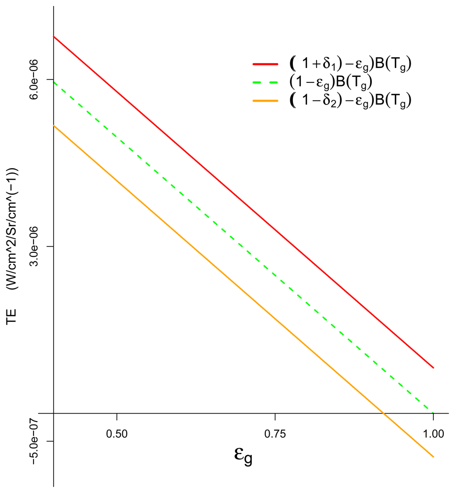
We present a plot of
TE as a function of
ϵg(
ν) for the three temperature cases at
ν = 1000 cm
−1 in
Figure 1. We set the ground temperature to
Tg = 300
K and vary the plume temperature at
Tp = 305, 300, 295
K.
The plots of TE for the Tp> Tg and Tp = Tg cases are the red and green lines, respectively. The plot shows that values of ϵg(ν) closer to 0 increase the magnitude of TE. This is consistent with the interpretation of the analyses.
The plot of TE when Tp < Tg illustrates which values of ϵg(ν) yield a larger TE in magnitude. We can see that TE crosses the horizontal axis if ϵg(ν) = B(Tp; ν)/B(Tg; ν). This shows that when ϵg(ν) = B(Tp; ν ν/B(Tg; ν), the plume is neither emitting nor absorbing and there is no chemical signal at wavenumber ν. The fact that TE can cross the horizontal axis informs us that small emissivities (closer to 0) or larger emissivities (closer to 1) have the potential to make the absolute value of TE larger for this temperature case.
The implications of this plot are as follows. When the gas exhibits an absorbance feature at wavenum-ber
ν and
TE is positive the plume is in emission. The analysis implies that backgrounds that have emissivities closer to 0 at wavenumber
ν will then contribute to a larger chemical signal, and thus the plume will be easier to detect. We note that this is true for each temperature case
Tp =
Tg and
Tp >
Tg. When
Tp <
Tg it is possible for
TE to be either positive or negative (plume is in emission
or absorption). This is illustrated by the orange line in
Figure 1. Thus, for this case, there are two ways that background emissivity can contribute to a larger
TE. If
TE is positive then emissivities closer to 0 yield a larger
TE and a larger chemical signal. When
TE is negative then emissivities closer to 1 may contribute to a larger chemical signal. Thus the plume will give some chemical signal for emissivities near 1 when
Tp <
Tg and
TE < 0 and this distinguishes this temperature case from those where
Tp ≥
Tg.
3. Experimental Methods
The goal of this section is to explore the validity of the analysis presented in Section 2. While the analysis describes the effect of ϵg(ν) on the chemical signal at a single channel, hyperspectral instruments record a radiance vector across the LWIR band. As such, we will explore how these phenomena affect gas detectability in a multivariate setting. To illustrate the claims made in the single channel analysis, we will restrict ourselves to a specific subset of gases and background emissivities. We choose gases that exhibit strong absorbance over a small range of wavenumbers and no absorbance everywhere else. We also select emissivities that do not change ordering over the wavenumbers where the gas exhibited absorbance. The intent is that illustrating the phenomena with gases and backgrounds that exhibit this relationship will allow for immediate interpretation of the results in relation to the model analysis provided in section 2. We intend to explore the effects of general background emissivity and gas absorbance variability on gas detectability in future work.
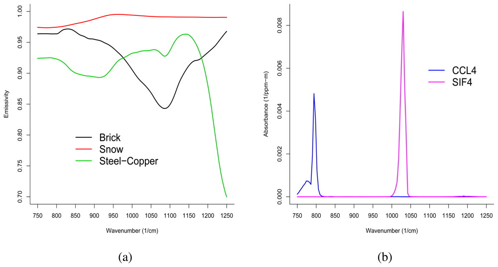
We employ IR-SAGE to simulate simplified hyperspectral images. The background spectra used in this study are laboratory-measured individual background materials from the Nonconventional Exploita-tion Factors Data System (NEFDS), a government database of surface reflection parameters. We selected three distinct background emissivity clusters and used the mean spectra of the three clusters in image simulation. These spectra are representative of the following three groups: Brick, Snow, and Steel-Copper Tubing. These spectra are presented in
Figure 2(a). Note that in the LWIR (750-1250 cm
–1), these emissivities are relatively high.
Two gases were selected for image simulation. We selected Carbontetrachloride (CCL
4) and Tetraflo-urosilane (SiF
4). These gases exhibit one large dominant absorbance feature. A plot of the absorbance spectra for these gases is presented in
Figure 2(b). The spectrum for CCL
4 shows a major feature around 790 cm
–1. SiF
4 exhibits a dominant feature around 1025 cm
–1. Note that the background emissivities show a consistent ordering across type (they do not cross) where each of the chemicals exhibits positive absorbance.
The simulated images have dimensions 75 × 120 × 126 (rows by columns by spectral dimension). The wavenumber range used is 750 to 1250 cm–1 in steps of 4. The three background spectra are inserted across the rows in three 25-pixel swaths. The chemicals are inserted as six 20-column bands at concentration pathlengths 16, 8, 4, 2, 1, and 0 ppm-m. This orientation produces 500 pixel replicates within a background/gas concentration combination.
Images were created for each temperature case. The ground temperature, Tg, was kept constant at 300K, and the plume temperature, Tp, was varied at Tp = 305K, 300K, and 295K for the CCL4 images. This temperature range was selected to illustrate the effect for each of the background emissivities on detection. A slightly wider temperature range was needed to illustrate the effect for SiF4: Tg = 300 and Tp = 305K, 300K, 292K.
Simulated sensor noise was used to perturb the spectra in each pixel. Variability due to atmosphere, temperature, and emissivity from pixel to pixel were held constant to enable us to study the effect of the background emissivity's variability across the spectrum on the chemical signal. IR-SAGE models sensor noise from a zero-mean Gaussian distribution with standard deviation defined by the ratio of sensor incident radiance to the signal-to-noise ratio. Please see [
8–
10] for detailed descriptions of the sensor noise model.
We use the Adaptive Matched Filter (
AMF) as a gas detector, note that this is equivalent to the gener-alized least squares solution to a linear model e.g. see [
1,
15]. The image analysis process is as follows. The non-gas pixels can be formulated as
where bold terms are vectors of length 126 (126 spectral channels) and ⨀ denotes the Hadamard product (elementwise multiplication;. We compute the mean of these pixels for use in background radiance subtraction. This can be represented as
for the 500 non-gas replicates as the atmospheric transmissivity and background radiance are not varied across pixels. We subtract this quantity from each of the gas pixels that contain the same background type, i.e., we compute
Eq. (16) shows how the background mean subtraction removes radiance due to ground as well as atmo-spheric upwelling radiance and leaves the chemical signal and noise. These data are processed with the
AMF. Explicitly we compute
where
A is a 126 × 1 vector of the gas absorbance spectra and ∑ˆ : 126 × 126 represents the spectral covariance matrix computed on the non-gas pixels. This formulation of the filter is sometimes used in practice in the LWIR. It assumes no information about the atmosphere, plume or ground temperatures, and emissivity is available. It also assumes that
TE is constant across the spectral dimension [
1,
2].
If the
AMF is deemed statistically significant based on a 5% level two-sided hypothesis test [
16], then we say we have “detected” the gas in that pixel. This test is conducted under the assumption that the errors follow a Gaussian distribution. We apply this solution to each of the 500 replicates within each gas concentration path-length/background combination and then record the proportion of detections:
We use pˆ as an estimate of the gas detection probability. We get 18 detection probabilities for each image as there are three backgrounds and six gas-concentration path-length levels. Lastly, we plot detection proportions versus concentration path length and look for orderings (conditioned on background emis sivity) in these curves. We then interpret these results back to the claims to the effect that background emissivities should produce a larger chemical signal and better detectability for each chemical.
4. Results
In this section, we present the results of analyses performed on the six synthetic images that were generated using IR-SAGE. Sample detection proportions were computed for each combination of con-centration path-length and background type. Taken together, these data form the empirical detection proportion curves presented in
Figure 3 (for CCl
4) and
Figure 4 (for SiF
4).
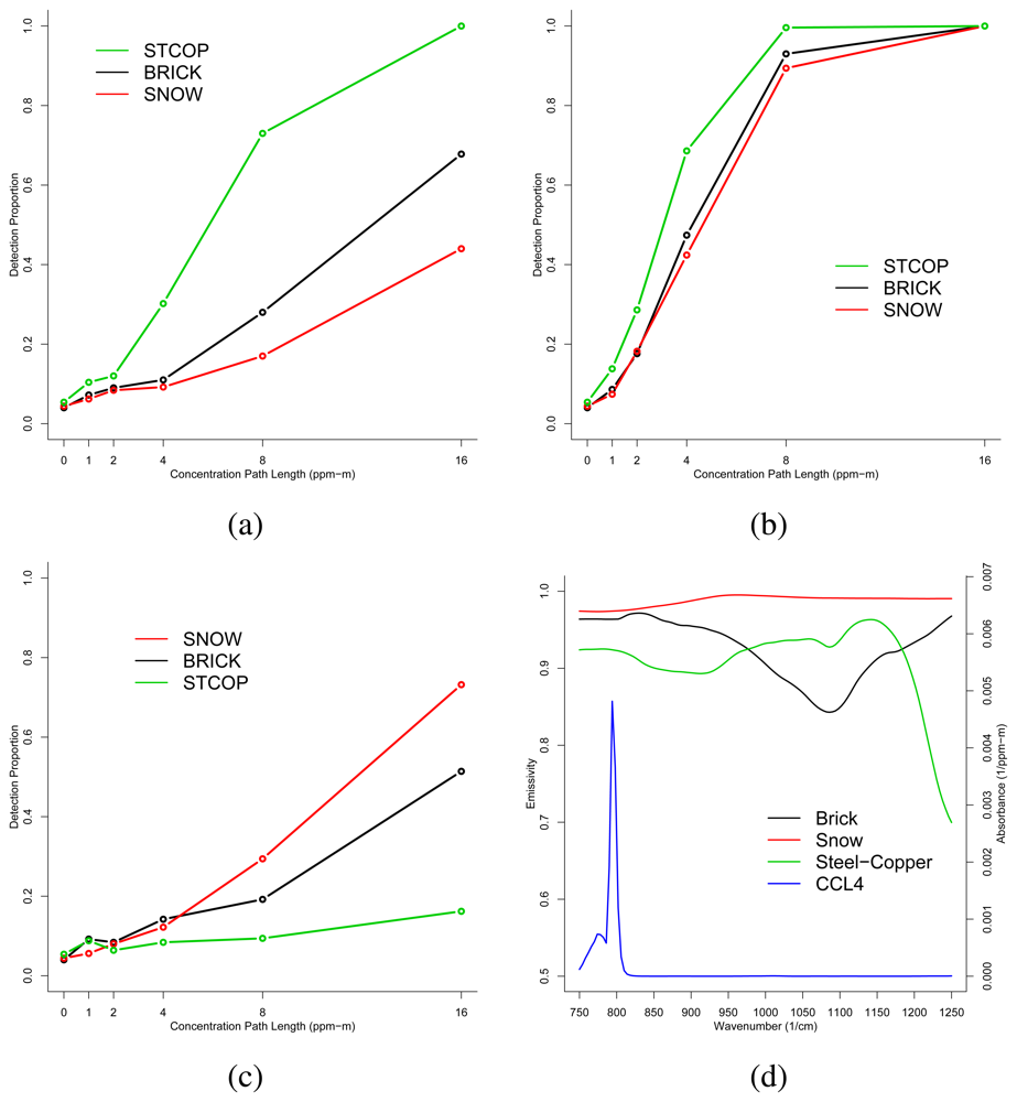
First, we consider
Figure 3(a), which is a plot of the empirical detection curves for CCL
4 when
Tp =
Tg = 300
K. Examination of the plot shows that the backgrounds can be ordered by detection proportion as (best to worst) Steel-Copper, Brick, and Snow.
Figure 3(d) shows a plot of the CCL
4 absorbance spectra along with the background emissivities. We see that where CCL
4 exhibits the large absorbance peak, the background emissivities can be ordered from low to high as Steel-Copper, Brick, and Snow. Thus, the results here are consistent with the characterization of
TE for this temperature case: lower background emissivities contribute to larger chemical signal when the plume is in emission.
Next, we consider the detection proportion plot for 305
K =
Tp >
Tg = 300
K in
Figure 3(b) which shows the same ordering in backgrounds as the previous temperature case. It also shows that detection has generally increased over all backgrounds. These observations are consistent with the characterization of
TE as they represent the fact that the backgrounds that give better detection for the
Tp =
Tg case are the same as for the
Tp >
Tg case. They also represent the fact that
Tp >
Tg gives a larger
TE and in turn a larger chemical signal.
Third, we consider
Figure 3(c), which shows the empirical detection curves for CCL
4 when 295
K =
Tp <
Tg = 300
K. Now we see that the ordering in the detection curves by background is Snow, Brick, and then Steel Copper. Inspection of
Figure 3(d) shows that the background emissivites can be ordered (high to low) as Snow, Brick, then Steel-Copper where CCL
4 exhibits its dominant absorbance peak. These results are consistent with the analysis of
TE for this temperature case. They illustrate that, for an absorbing plume and a large enough (negative)
TE, the backgrounds that give best detection are those that exhibit larger emissivities and not smaller ones as in the previous two temperature cases.
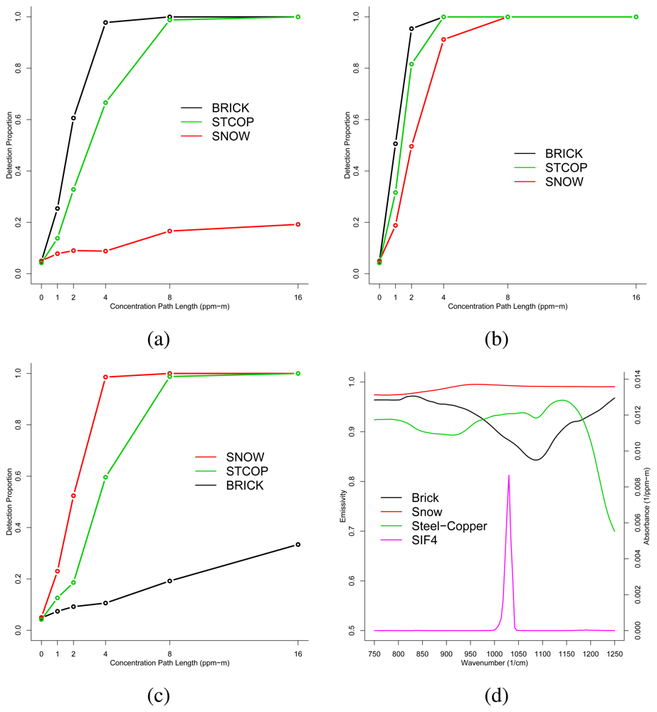
Now we consider
Figure 4(a), which is a plot of the empirical detection curves for SiF
4 when
Tp =
Tg = 300
K. Examination of the plot shows that the backgrounds can be ordered from best to worst detectability for SiF
4 as Brick, Steel-Copper, and Snow.
Figure 4(d) shows that the background emissivities can be ordered from least to greatest as Brick, Steel-Copper, and Snow where SiF
4 exhibits its dominant absorbance peak. This ordering is consistent with the analysis of
TE: smaller emissivities yield a larger chemical signal for this case.
Next, we consider
Figure 4(b), which gives the SiF
4 detection proportions when 305
K =
Tp >
Tg = 300
K. Examination of this plot shows that the background orderings by detection proportion are the same as the
Tp =
Tg case. The plot also shows that detection has generally increased for the emitting plume at a higher temperature.
Last, we consider the plot in
Figure 4(c), which presents the empirical detection proportions when
Tp= 292
K <
Tg = 300
K. This plot shows that the backgrounds that yield best detection have changed ordering to Snow, Steel-Copper, and Brick. Again, we see that larger emissivities yield larger detection proportions for a large
TE when
Tp <
Tg.
5. Conclusions
The effects of clutter on gas plume detection/identification is a complicated problem that is ap-proached from multiple perspectives. This paper studied the effects of background emissivity and plume/ground temperatures on the chemical signal. The analysis is most pertinent to treatments of the physics-based radiance model that linearize the plume transmissivity term and work with linear ap-proaches to gas detection or identification.
Our investigation has shown that, when ignoring reflected downwelling radiance, the physical state of the plume (emission, neutral, or absorption) is not only dependent on the plume/ground temperatures, but is also directly dependent on the background emissivity, ϵg (ν), at a particular wavenumber. We have shown that Tp ≥ Tg implies that the plume is strictly in emission and that values of ϵg (ν) closer to 0 will contribute to a larger observed chemical signal. Further, when Tp < Tg, we have shown that it is possible that the plume is in emission, absorption, or neither emitting nor absorbing (neutral). A neutral plume happens when ϵg (ν) = B(Tp; ν)/B(Tg; ν). Thus, the background has the potential to completely obscure the plume at wavenumber ν. The analysis also shows that emissivities closer to 0 or 1 in this case have the potential to contribute to a larger observed chemical signal.
The analysis was verified by analyzing simulated hyperspectral radiances in the absence of atmo-spheric, background, and temperature variability. The gas absorbance and background emissvities used in image simulations exhibited a very strong relationship: the background emissivity ordering did not change over the wavenumbers that exhibited gas absorbance. This made it possible to illustrate the re-sults of the model analysis in a multivariate setting. In general, real background emissvities and gas absorbances will not exhibit this relationship, so we aim to further explore this phenomenology while allowing the gas absorbance and background emissivity to vary across the entire LWIR portion of the spectrum.


