Vertex Separators for Partitioning a Graph

Department of Software Engineering, Faculty of Computer Sciences, Izmir University of Economics, 35330 Balcova, Izmir, Turkey
Sensors 2008, 8(2), 635-657; https://doi.org/10.3390/s8020635
Submission received: 5 December 2007
/
Accepted: 29 January 2008
/
Published: 4 February 2008
(This article belongs to the Special Issue Energy Efficiency and Intelligent Signal Processing for Wireless Sensing)
Abstract
:Finite Element Method (FEM) is a well known technique extensively studied for spatial and temporal modeling of environmental processes, weather prediction computations, and intelligent signal processing for wireless sensors. The need for huge computational power arising in such applications to simulate physical phenomenon correctly mandates the use of massively parallel computers to distribute the workload evenly. In this study, a novel heuristic algorithm called Line Graph Bisection which partitions a graph via vertex separators so as to balance the workload amongst the processors and to minimize the communication overhead is proposed. The proposed algorithm is proved to be computationally feasible and makes cost-effective parallel implementations possible to speed up the solution process.
1. Introduction
Finite Element Methods (FEM) and repeated solutions of linear systems of equations for different right-hand side vectors in the form of Ax=b where A is, often, a sparse matrix, and x and b represent the unknown solution and mismatch vectors respectively have been used extensively for spatio-temporal modeling of solar radiation [1], climate [2,3,4], environmental [5] and biogeochemical changes [6], as well as in diverse fields such as Simultaneous Localization and Mapping (SLAM) [7,8] and VLSI design [9]. The need for huge computational power arising in such applications to simulate complicated physical phenomenon accurately, on the other hand, demands the use massively parallel computer architectures. These architectures with many nodes capable of performing computations autonomously have a versatility of design alternatives as to the topology of the network amongst individual nodes for communication. A balanced distribution of the total workload imposed by such an application amongst the available processors of a parallel computer has been shown to be the key element in achieving high speed-ups.
The issue of distributing the overall workload evenly amongst a set of processors has been widely studied [9-18] as a graph partitioning problem. This, in its general form, requires dividing the set of nodes of a weighted graph into disjoint sets such that the sum of weights of nodes in each subset is almost the same and the total weight of all of the edges connecting nodes in different partitions is minimized. The constraint of balancing over all subsets of the total weights corresponding to individual workloads of processors provides for a higher degree of parallelism, and hence, a minimized overall completion time, while the latter helps to decrease the amount of interprocessor communications by minimizing the sum of edge weights amongst different partitions. Depending on the type of the applications, partitioning is performed by a removal of either a small set of edges or a small set of nodes.
In this paper, a novel heuristic algorithm called Line Graph Bisection to partition a graph by the latter approach, namely, node separators, is developed. The proposed algorithm is shown to be readily applicable within existing frameworks of graph partitioning, and also, proven to be computationally feasible. The paper is organized as follows: Section 2 presents a formal description of the nodal graph partitioning problem. Survey of the related work, and motivations that led to the development of the algorithm developed in this study are given in Section 3. Section 4 describes the proposed algorithm in detail and proves that it is computationally feasible. In Section 5, a comparative analysis is performed on the qualitative grounds and based on some test cases. A mapping scheme for parallelization is presented in Section 6. The paper is, finally, concluded and also some future research directions are specified in Section 7.
2. Nodal Graph Partitioning
Given an undirected graph G = (N,E) where N is the set of nodes, and E denotes the set of edges linking nodes, this study aims at partitioning it into clusters with vertex separators between them, and later, assigning each cluster to a processor such that the overall simulation time is minimized. Without loss of generality, the graph G is assumed to be connected. A vertex separator is defined to be a set of nodes S ⊆ G whose removal divides the graph into two disconnected components. Both the computational and communicational load in each processor must be optimized to achieve this goal. To this end, this study states two important optimization criteria: (1) load balancing and (2) separator minimization. The latter helps to minimize the interprocessor communication while increasing the amount of parallelism and reducing the number of sequential operations needed in the separator. Finding minimal size vertex separators was shown to be NP-Hard even in graphs with nodes having a maximum degree of three [19]. Since finding an optimum partitioning for a given graph is an intractable problem, this study proposes a novel heuristic approach called Line Graph Bisection (LGB) algorithm.
3. Related Work and Motivations
There has been tremendous research on graph partitioning in the literature. Liu and Ashcraft [21] have classified them into two different categories: (1) direct approaches which construct partitions and (2) iterative approaches which improve them. Direct approaches include nested dissection algorithm [13,15] based on alternating level structures and spectral methods [22]. Kernighan-Lin algorithm [9] and its variant [11] use, on the other hand, an iterative approach by either swapping vertices between the existing partitions or moving a vertex from one partition to the other. Another example of an iterative approach is given in Liu's work [16] based on bipartite graph matching. This work has later been extended by Liu and Ashcraft [21] using a method that very much resembles to a version of Kernighan-Lin algorithm that operates directly on a vertex separator by moving nodes to and from the corresponding partitions this time.
There exist some other algorithms which have relied on the underlying characteristics of the problem domain. One such algorithm that arises in applications where the graph is planar was studied by Lipton and Tarjan [23]. As planarity of the graphs representing different problem domains is not often preserved, such existing methods are not normally expected to produce good load-balanced partitions with minimal separator size. Duff et al. [12] have provided an interesting discussion of an automatic partitioning in the context of reordering and pointed out that there are no partitioning algorithms that are presently in common use with a sparse matrix package.
It is emphasized in [24] by Hendrickson and Rothberg that finding an edge separator first, and then, trying to obtain a vertex separator from it typically based on a matching technique are only indirectly related to the quantity that should actually be minimized. A combination of local improvement techniques is, however, noted to be more effective [24]. Pothen, in [25], describes the use of Kernighan-Lin algorithm in the post processing stage of different implementations as a good refinement policy. Karypis and Kumar [26] have used a variant of Kernighan-Lin for refining the results obtained by a multilevel partitioning scheme and proved that it was effective. Gupta [10] has presented another example of a partitioning framework which incorporates Kernighan-Lin algorithm in its refinement phase. Gupta [10] has also reported that the assumption of the size of a node separator being proportional to the size of the edge separator containing it was often incorrect, especially, for highly unstructured linear programming matrices.
Kernighan-Lin algorithm as an edge separator minimizing bisection algorithm can be seen to find its niche in refining results obtained via a versatility of algorithms and frameworks proposed in the literature. This observation coupled with the fact that constructing vertex separators from edge separators is not always effective forms the primary sources behind the motivation for LGB algorithm devised in this study. LGB is, hence, developed to obtain vertex separators directly, and yet, has the same characteristics as does Kernighan-Lin (KLB) algorithm so that it is readily applicable to domains where KLB is currently being used. The objective stated may as well hint to the idea behind LGB. If KLB could be somehow modified without imposing any constraints on the way it operates in such a way that it would be possible to treat the nodes as if they were edges, LGB would find its uses in graph partitioning through vertex separators both as a better replacement for KLB when used in the refinement phase and as a standalone heuristic algorithm which may be coupled with other combinatorial techniques to produce more powerful schemes to better suit the needs of different domains.
4. Line Graph Bisection Algorithm
Line Graph Bisection algorithm has been inspired from the well-known Kernighan-Lin [9] graph bisection algorithm (KLB) by incorporating some novel modifications so as to make finding vertex separators possible. KLB finds small edge separators in O(n2 log n) time where n denotes the number of nodes in the graph. Fiduccia and Mattheyses [11] improved this running time to O(|E|). Before the details of LGB algorithm that finds small vertex separators directly are given, some new terminologies used throughout the paper are first introduced briefly.
4.1 Terminology
Definition 4.1: A Line Graph L(G) (also called an interchange graph) of a graph G is obtained by associating a vertex with each edge and connecting two vertices with an edge if and only if the corresponding edges of G meet at one of the either nodes that are endpoints.
Let us assume that we have a graph of which all the nodes are numbered and all the edges are labeled distinctly. In this case its line graph is the graph obtained by replacing each edge with a corresponding single node and each node with some number of edges proportional to the degree of the respective node. An example graph G and its corresponding line graph L(G) are depicted in Figure 1.
As can be seen from Figure 1, since there exists at most one edge between two different nodes in the original graph G, every node in L(G) will have edges emanating from it labeled by one of the two distinct labels corresponding to the two nodes it connects in G. Let us consider the edge labeled 3-4 in G in Figure 1a. It can be seen that all the edges incident on node 3-4 of L(G) in Figure 1b are labeled by either 3 or 4 which are the nodes linked by the corresponding edge in G.
Terminal nodes in the original graph, on the other hand, with a degree of one will be edges in the line graph represented with one of their end points as a non-existent artificial node. It should also be noted that artificial nodes in L(G) (see Figure 1) are just for the sake of completeness and do not have a corresponding edge in the original graph G.
Definition 4.2: Labeled degree of a node in a line graph L(G) is defined as the total number of the distinct labels of the edges incident on this node.
Theorem 4.3: The labeled degree of each node that is not artificial is exactly two in the line graph.
Proof: It follows easily from the definition of line graph and Definition 4.2. Each node n with the exception of artificial nodes in L(G) corresponds to a unique edge e connecting nodes x1 and x2 in the original graph G. The only possibility for node n to be connected to other nodes in L(G) is therefore through edges labeled either x1 or x2 which correspond to nodes x1 or x2, respectively in G.
It can easily be derived from Theorem 4.3 that there exists no degree one vertex in a line graph with the exception of artificial nodes. This fact is presented in Lemma 4.4.
Lemma 4.4: There exists no degree one vertex in a line graph.
Proof: Q.E.D by the above stated fact.
Having introduced the terminology, the KLB algorithm whose understanding is crucial to the development of the proposed (LGB) algorithm can be described now.
4.2 A Close Look at the KLB Algorithm
The Kernighan-Lin algorithm [9] is a well-known graph bisection heuristic and finds small edge separators in O(n2 logn) time where n is the number of nodes in G. Succeeding discussions in this section of the paper refer to a more efficient version of KLB described in [11] where Fiduccia and Mattheyses improved the running time to O(|E|), since the proposed LGB algorithm is also based on that version of KLB implementation found in [11].
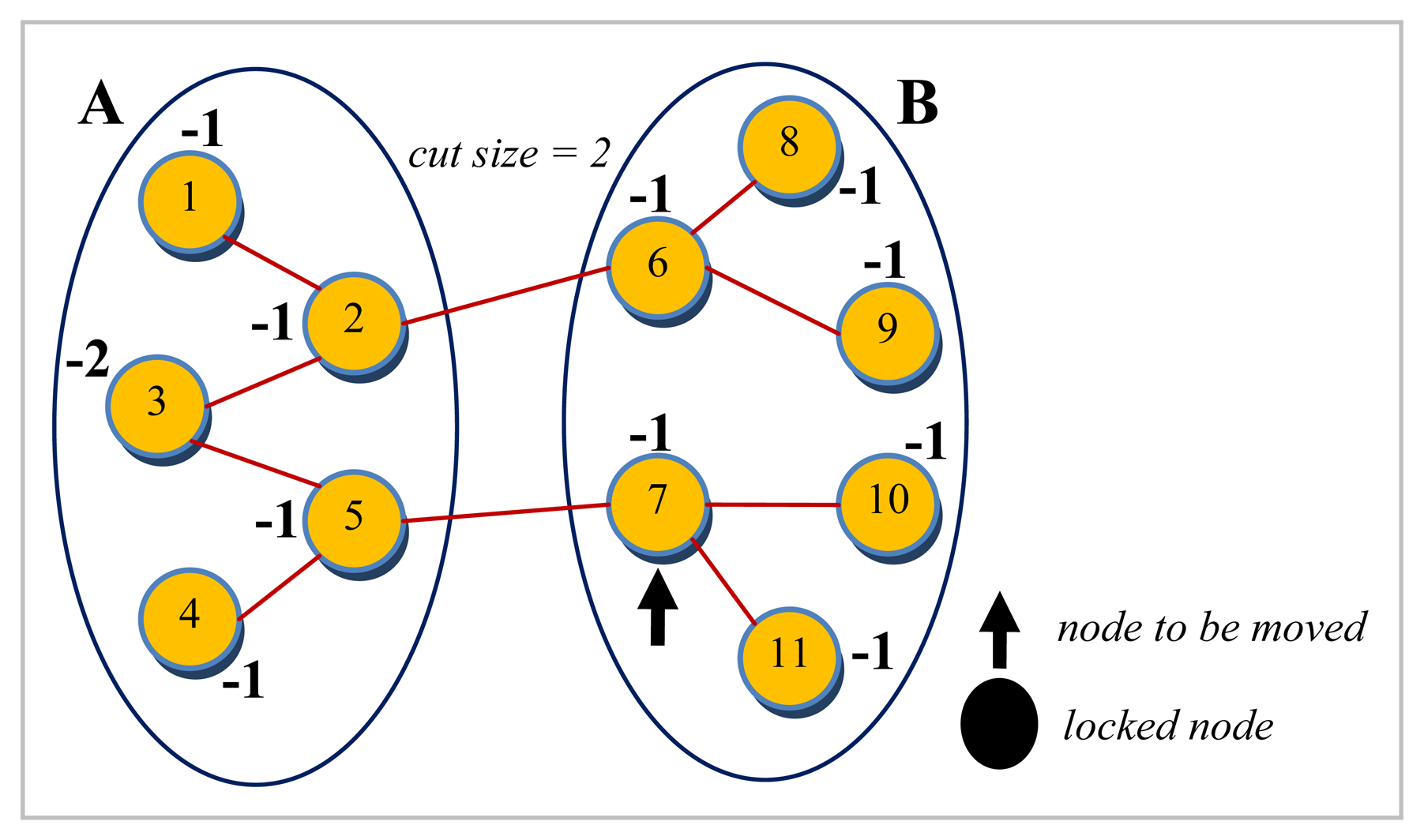
In order to partition a graph into two clusters such that the total weight of the edges in the cut, i.e., between the two partitions, will be minimized, and the sum of the node weights in each of the two partitions will only differ by a tolerance factor, the graph is initially partitioned into two randomly chosen sub-graphs. Then, by a number of moves originating from the partition with more total weight to balance the load implicitly, the cut size (the sum of the weights of edges from one partition to the other partition) is tried to be made smaller. To perform such a task, the node to be selected in each move should be the one which has the maximum gain. The gain of a node in the KLB algorithm is defined as the total weight of edges by which the cut size would increase or decrease if this node were to be moved to the other partition. Each node in a given configuration has some internal and external edges (i.e., some link to those vertices in the same partition, and others to those in the other partition, respectively). The gain of a node ni, say in partition A, to be moved to partition B is thus defined as follows:
where w(i, j) denotes the weight of an edge between nodes ni and nj. This is exactly equivalent to the total weight of external edges minus the total weight of internal edges incident on node ni. An initial partition by KLB is shown in Figure 2, with all the gain values already calculated. For the sake of the ease of representation in Figures 2 and 3, it is assumed in this example that all the edges have a weight of one. This causes the gain calculations to be reduced to be simply the difference of the number of external and internal edges. Since partition B has more number of nodes as shown in Figure 2, a node with the maximum gain value belonging to this partition is chosen. If there are multiple candidates with same gain value, the tie can arbitrarily be broken. After the move is performed, the gains of other nodes need to be updated to account for the displacement caused by this move. The reason that this process is quite straightforward in KLB is two folded: First, calculating the gains of just the adjacent nodes is sufficient since they are the only ones affected by the move. Second, the gains of the adjacent nodes need not be computed from scratch as they can easily be updated based on the knowledge of prior gain values. Each neighbor nj of the moved node ni if external now has a gain of gainold + 2w(i, j), and those which are in the same partition now have a new gain equal to gainold – 2w(i, j) where w(i, j) is the weight of the edge between nodes ni and nj. The moved node is, finally, locked not to be moved once again. Figure 3 depicts the configuration reached after node 7 after it is moved to partition A and locked there.
The process continues until all the nodes are locked. To prevent the procedure from getting stuck at a local maximum, the sequence of moves that gives the maximum total decrease in the cut size is chosen afterwards. This, in turn, means that some intermediary individual moves that may even worsen the cut size are allowed. All the nodes are unlocked at the end of the iteration, and the sequence of moves minimizing the cut size is actually performed this time, thus resulting in a new configuration, and the algorithm is restarted with this new initial configuration. The overall procedure may be repeated so long as either the cut size decreases or the load balance is improved.
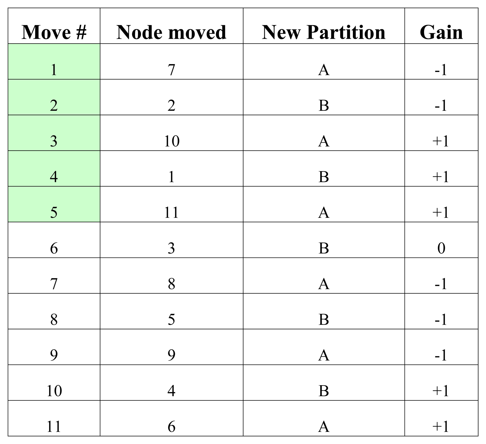
Figure 4 lists the moves performed by KLB for the example initial configuration given in Figure 2 and iterated in Figure 3. Cut size is initially equal to 2 as can be seen in Figure 2. Moves 1 through 5 are performed to maximize the total gain resulting in a cut size of 1. This algorithm as described is simple and fast.
In the next section, how the proposed algorithm, LGB, has evolved will be explained, and it will be presented in detail.
4.3 LGB Detailed
The trick which makes the LGB algorithm possible is to convert the original graph G into its corresponding line graph L(G). The property that the edges of the line graph correspond to the nodes of the original graph enables us to design a new heuristic algorithm which once more finds small edge separators but in the line graph this time. This, in effect, allows us to directly obtain vertex separators for the corresponding original graph.
The LGB algorithm is, in essence, a modified version of KLB in that both the characteristics of the line graph such as the existence of edges, now, that needs to be treated as one and the requirements imposed by the original problem such as the necessity to keep track of the loads of the respective partitions in terms of the weights of the edges rather than nodes are neatly taken into account so as to efficiently compute small edge separators. Assuming that such small edge separators can feasibly be found in the line graph through an algorithm which is going to be described in full detail shortly, it is trivial to derive the corresponding nodal partition induced in the original graph which corresponds exactly to the minimum cut partition obtained by LGB in the line graph.
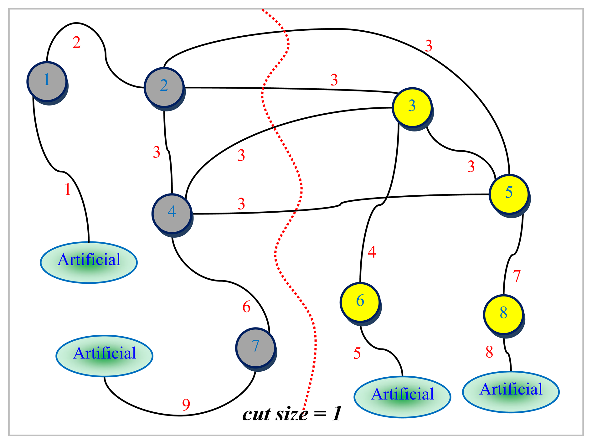
An example graph G for which a small size vertex separator is sought and its corresponding line graph L(G) are depicted in Figures 5 and 6, respectively. The numbers shown next to each edge in Figure 5 are used to uniquely identify them. All the nodes are assumed to be associated with a weight of one for the example graph G given in Figure 5. The dotted line in red seen in Figure 6 represents the bisection of L(G) computed by the LGB algorithm. There are a total of four edges in the cut in Figure 6. These edges have been all labeled the same (i.e., 3 corresponding to node 3 in Figure 5). It can easily be seen from Figure 6 that nodes 1, 2, 4 and 7 shaded in grey together with edges 1, 2, 3, 6, and 9 of L(G) to the left of the dotted line in red are all pinned in a separate partition. These grey-shaded nodes 1, 2, 4, and 7 in Figure 6 are actually the edges labeled as 1, 2, 4, and 7 again, respectively in Figure 5. The edge separator and the partitioning scheme in Figure 6 obtained by the LGB algorithm, thus, induce the nodal partitioning specified by the configuration of Figure 5 in which only node 3 ends up in the separator. While nodes in grey (1, 2, 6, 9) are assigned to a partition, nodes in yellow (4, 5, 7, 8) are placed in another which turns out, in this case, to be an optimal vertex partition with respect to both the separator size minimization (just node 3) and the load balance (each have 4 nodes) constraints. It should, however, be noted at that point that the cut size has been treated as one in Figure 6 by counting only the number of distinct labels of weight one as specified by the example at the cut. As it is quite clear from the discussion of the example, LGB is a modified KLB applied to the line graph. The only modifications needed, apparently, are those which stem from the fact that a number of edges having the same label in the line graph have to be treated as a single edge and the fact that the partition weights implicitly used to control the quality of load balance are, now, a function of the edge weights rather than the node weights. The existence of multiple edges having the same labels in the line graph as seen in Figure 6 has a direct effect on the way the gain of a node is calculated and updated in the line graph. The efficiency of the proposed LGB algorithm heavily depends on preserving the locality of updates in LGB as is the case in KLB.
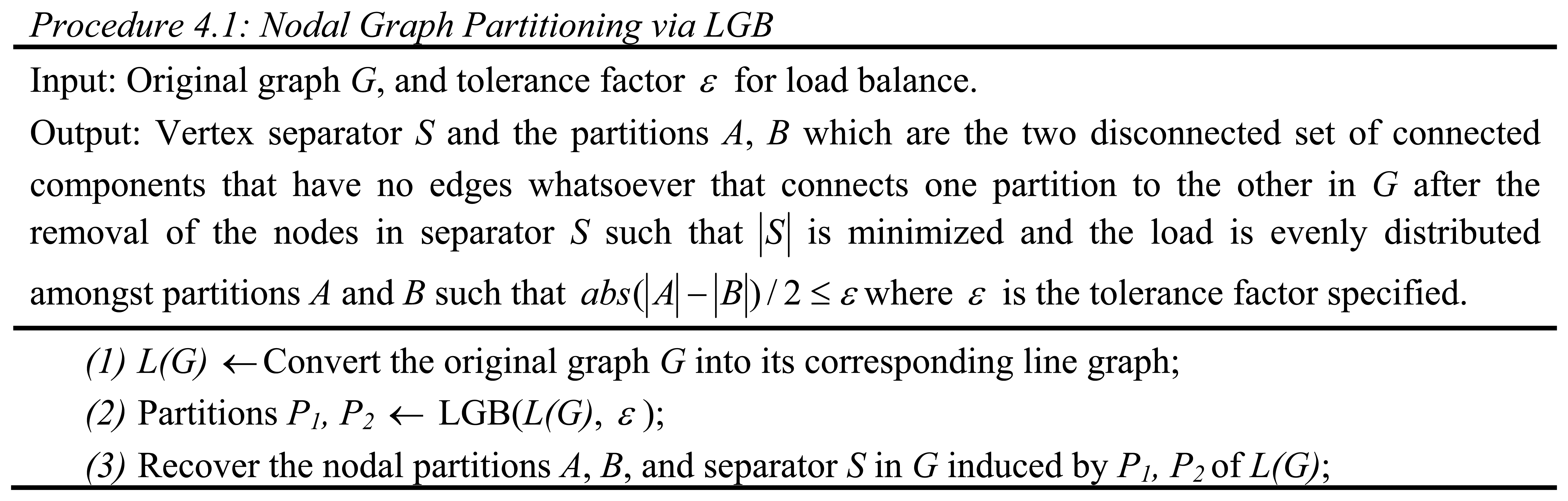
In light of the previous discussion, the overall procedure for partitioning a graph via vertex separators may be formulated as listed in Figure 7.
For computing vertex separators as outlined in Figure 7, the original graph G is first transformed into its line graph equivalent L(G). The LGB algorithm is, then, applied to obtain the partitions P1 and P2 similar to the KLB algorithm. The only exception is, this time, that gain value calculations and updates take place with respect to the labeled edges grouped into two for each node. The vertex separator and the corresponding partitions are, finally, recovered in G as dictated by the partitioning scheme induced by P1 and P2 of L(G) obtained by an application of LGB. As the corresponding line graph of the original graph has now been partitioned into clusters such that the sum of the weights of the edges with distinct labels across clusters is minimized and the load of each cluster is balanced up to a tolerable amount, the total weight of the vertices in the separator of the original graph corresponding to the distinct labels of the edges in the cut of its line graph have also been minimized effectively. A similar argument holds with respect to the balancing of load over the partitions so long as a modification is incorporated into LGB such that the sum of all the individual weights of the labels in the set of distinct labels of edges instead of the total weight of nodes in respective partitions of L(G) at any time is used to keep track of the individual weights of the partitions. Such a modification, which certainly frees us from assuming that the number of edges and vertices in the original graph are linearly proportional, is possible as will be explained shortly. The load is, therefore, balanced by LGB up to an amount specified by the tolerance factor ε.
The individual steps of Procedure 4.1 for computing vertex separators given in Figure 7 are detailed next in the following subsections.
4.3.1 Converting the Original Graph into its Line Graph
An algorithm to convert a given graph G into its corresponding line graph L(G) is sketched in [20]. The fact stated in Lemma 4.5 hints to the implementation of the line graph conversion algorithm used in step (1) of Procedure 4.1.
Lemma 4.5: The incidence matrix CG of a given graph G and the adjacency matrix JL(G) of its line graph L(G) are related by JL(G) = CGTCG − 2I where I is the identity matrix [20].
Lemma 4.6 given below is used to show the time complexity of the line graph conversion algorithm used.
Lemma 4.6: The line graph L(G) of a graph G with n nodes, e edges, and vertex degrees di contains n′ = e nodes and
edges [20].
Lemma 4.7: The running time complexity of the algorithm to find L(G) is O(e2) in the worst-case scenario and it is optimal.
Proof: The first for loop for labeling the edges takes
iterations where di is the degree of node i ∈ {1..n}. The second for loop for constructing the same labeled edges, on the other hand, is repeated as long as
times in the worst case. Thus, the algorithm has a running time proportional to O(e2) which completes the proof of the first part. The latter expression is simply the number of edges in L(G) given in Lemma 4.6. Hence, the number of edges in L(G) forms clearly a lower bound on the algorithm's time complexity. This, in turn, renders the algorithm optimal.
4.3.2 LGB Algorithm and the Data Structures
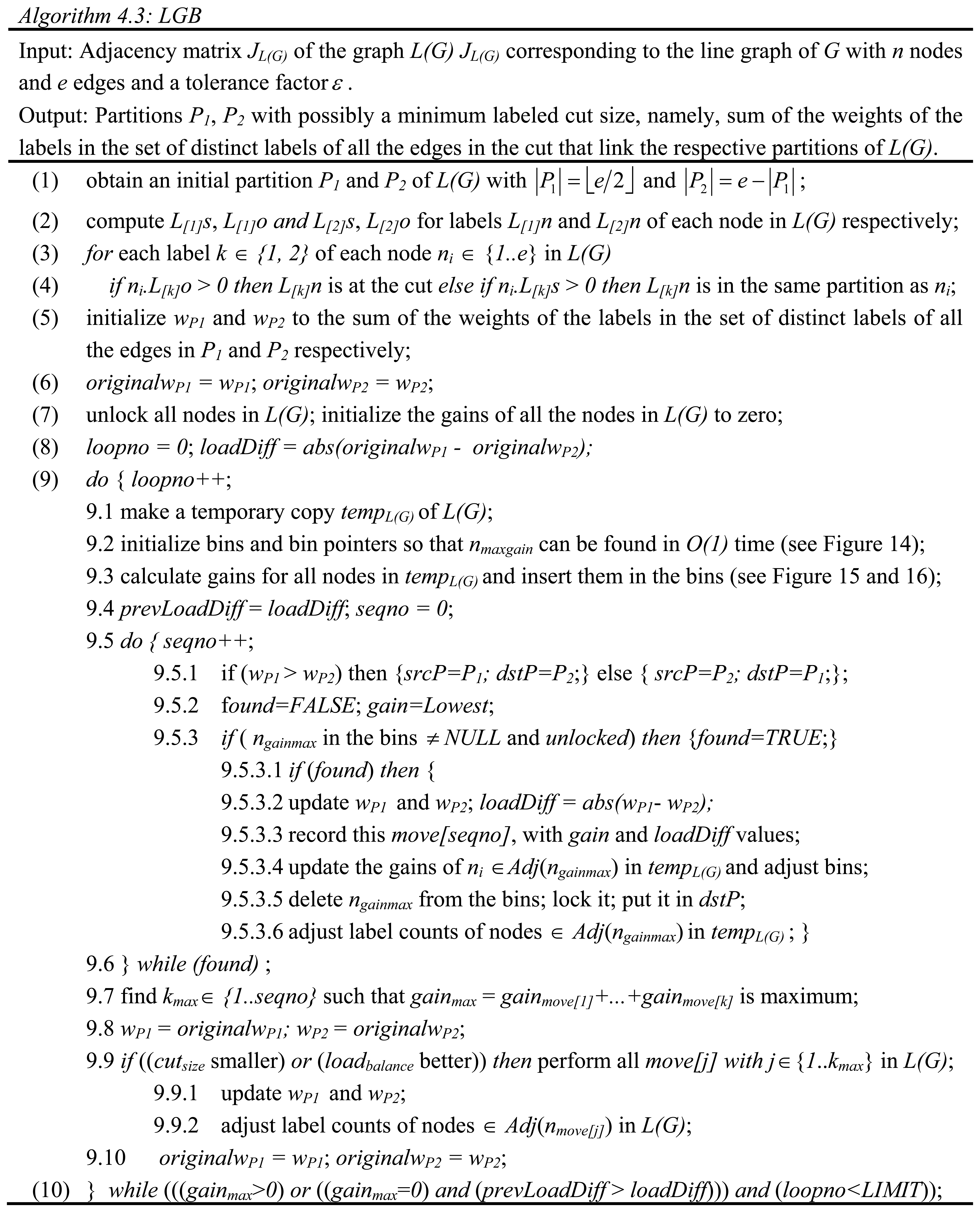
The LGB algorithm used in step (2) of Procedure 4.1 to find small vertex separators for partitioning a graph is listed in Figure 8. Both the data structures used and the algorithm itself are described next in the execution order as explanations are provided in detail.
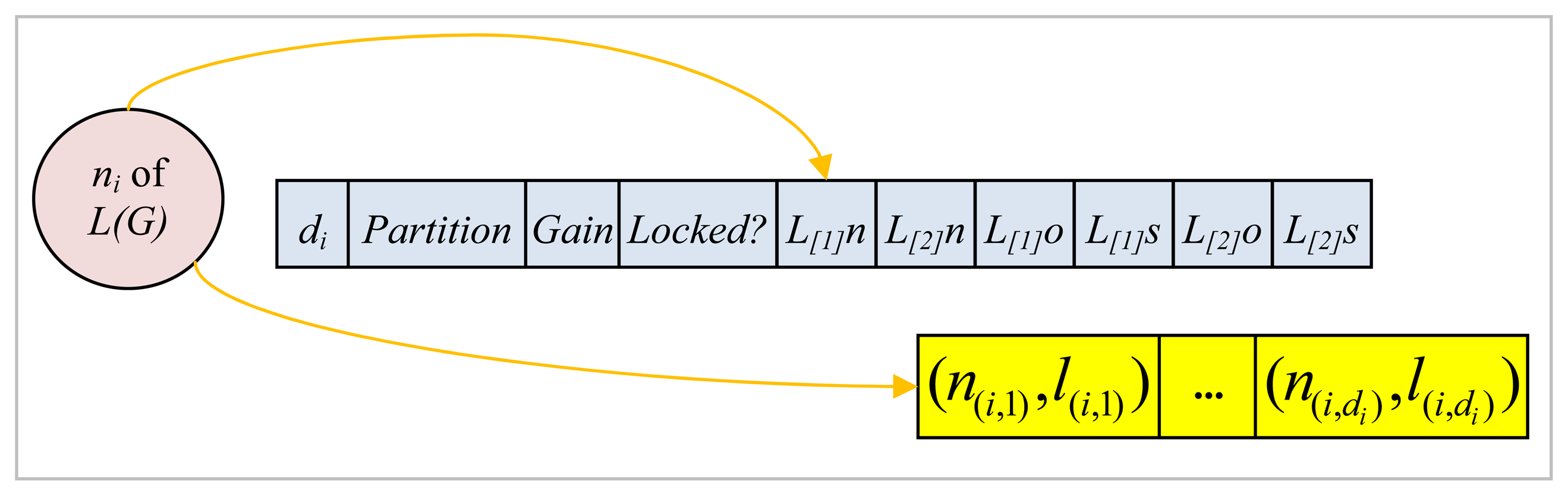
The input to the Algorithm 4.2 listed in Figure 8 is the line graph L(G) of the original graph G. L(G) is represented as an array of size e which corresponds to the number of edges in G.
Each slot of the array as shown in Figure 9 stores information for the corresponding node ni of L(G), such as its degree di; the partition it belongs to which may be either 1 or 2 at any instant corresponding to the two partitions P1 and P2, respectively; its gain value; whether it is locked or not at any instant; its L[1]n and L[2]n which stand for the names of the two distinct labels of the edges incident on this node; its L[1]s and L[2]s which denote the number of adjacent nodes connected with an edge labeled either L[1]n or L[2]n respectively that belong exactly to the same partition as the node under consideration; and L[1]o and L[2]o which are the number of adjacent nodes connected with an edge labeled either L[1]n or L[2]n, respectively, that are, on the other hand, located in the other partition with respect to the node at hand. Each node ni also points to an array of length di where a sequence of pairs in the form of (n(i,j), l(i,j)) where n(i,j) is an adjacent node and l(i,j) is the label of the corresponding edge are stored as shown in Figure 9.
Upon getting the input, LGB obtains an initial partition P1 and P2 at step (1) of the Algorithm 4.2. Depending on the initial partition, the number of external and internal edges for each of the two distinct labels, namely, L[1]o, L[2]o, L[1]s, and L[2]s, are calculated next by a single pass over the line graph L(G). Steps (3) and (4) detect the set of distinct labels in the cut as well as in partitions P1 and P2. This is, in effect, equivalent to finding the vertex separator S and partitions A and B of G induced by the partitioning of L(G) obtained initially. It is now time to calculate the initial weights of the partitions P1 and P2 and store them as original weights as outlined in steps (5) and (6) before the iterations start. In step (7), all the nodes are marked as unlocked so that they will have a chance of being moved and their gains are all initialized to zero. The initial load difference corresponding to the initial partition is stored at step (8) and the main outer loop starts at step (9) of the algorithm which can be iterated so long as the limit specified by LIMIT in line (10) is not exceeded and either the cut size or the load balance can be improved upon. LGB is just like Fiduccia and Mattheyses modified KLB, running with the exception that edges with the same label are treated as a single edge with the specified weight with respect to both the cut size and gain calculations performed. At step 9.1 of the outer loop between (9) and (10), a temporary copy of L(G)'s header section excluding the adjacent nodes shown in Figure 13 is created so that the results of intermediate moves can be recorded. Step 9.2 initializes the bins used for sorting the gain values of the nodes to make it possible to find maximum gain values in both partitions P1 and P2 in O(1) time via a process called bin sorting.
A doubly linked list data structure, Binspack, shown in Figure 10 has a slot for every node of the L(G). It has some fields in every slot for maintaining the current gain values of the corresponding nodes and two pointers named previous and next as shown in Figure 10 which point to the previous and the next nodes with the same gain values, respectively. If there is no previous node, however, previous is assigned the negative of the bin number pointing to this specific node whose gain value is directly related to the bin number in Binsptr data structure also shown in Figure 10. Binsptr[gv] [2] data structure is used to store the pointers to the first node in Binspack with a gain value equal to gv for each different gain value gv that can possibly be attained by the nodes in P1 as well as in P2 at all times during the algorithm. These two data structures enable us to find the node with the maximum gain value in each partition and also update the gains of the adjacent nodes that are affected from a move at each iteration in O(1) time by keeping the bins sorted. In case it is assumed that the nodes of G have all a unit weight equal to one, the corresponding edges of L(G) would, accordingly, have labels whose weights are also one. This would specifically induce a set of five possible gain values in the range of - 2 through 2 since each node of L(G) has two distinct labels and the move of such a node may either increase or decrease the cut size by none, one or both of the labels depending on the current configuration. Binsptr[i] [j], assumingly, would point to a node in the Binspack data structure with a corresponding gain value of (i-3) when i can take on values in the range 0 through 4. However, it should be noted at this point that in the general case where nodes in G=(N, E) may have different weights, possible integral values can be in the range specified by [−gν, +gν] where gν = 2 max{weight(ni)|ni ∈ N}.
Initial gains are calculated for all nodes in tempL(G) and inserted into the bins at step 9.3 right before the inner loop 9.5 - 9.6 of the algorithm starts moving the nodes. Since each node in L(G) has a labeled degree of two (see Theorem 4.3), the edges emanating from a node can virtually be grouped into two distinctly labeled sets: (1) those labeled by L[1]n and (2) the rest labeled by L[2]n, respectively.
Each set of edges naturally connects to some adjacent nodes that are either in the same partition called s or in the other partition called o as seen in Figure 11 with respect to the node whose gain value is to be calculated.
Definition 4.8: The set of the distinct labels of the edges whose endpoints are not both in the same partition is called the labeled cut set denoted by ℜ within the context of LGB.
Definition 4.9: The sum of the weights of labels in ℜ at any time is called the labeled cut size and denoted by Γ.
Definition 4.10: Gain of a node at any instant of LGB algorithm is defined as the change in the labeled cut size when the node is moved to the other partition.
The Algorithm 4.3 for calculating the initial gain of a node is given in Figure 12. There are only three cases to be considered for each node whose gain value is to be calculated. The fact that there are actually no more than only three cases can easily be deduced based on Property 4.11.
Property 4.11: If i is a node in the original graph and its degree is k, then k nodes in its line graph will be fully connected by the i labeled edges forming a clique. So the total number of the nodes in a clique connected by the same labeled edges are exactly k*(k-1)/2 in the line graph. This, in turn, implies that if there is an edge labeled ℓ between nodes t1 and t2, t3 has an edge also labeled ℓ incident either on t1 or t2, then there must exist other ℓ labeled edges from t3 to both t1 and t2.
The term weight(L[k]n) in Figure 12 refers to the weight of a node in G which labels the corresponding edges in L(G).
After recording the previous load balance difference at step 9.4, the inner loop that performs a sequence of moves from the source partition to the destination partition which has less weight until all the nodes are marked as locked is executed at steps 9.5 through 9.6. For each prospective move found, respective weights of the partitions are updated at step 9.5.3.2 of Algorithm 4.2 as detailed by Algorithm 4.4 shown in Figure 13.
Having recorded the move together with its sequence number, gain and the new load difference value between the partitions at step 9.5.3.3, it is time for updating the gains affected by this move at step 9.5.3.4. Fortunately, the nodes whose gains need to be updated are only those adjacent to the node just moved. Additionally, the updates are local in that the distinct labels in the cut need not be searched for updates to be done accurately.
Lemma 4.12: There is no need to keep track of the labels in the cut so as to figure out which labels are in the cut after a legal move in L(G).
Proof: The existence of a label in the cut can be instantly discovered according to Property 4.11 when both the number of edges linking to nodes in the same and the other partition are known a priori. The latter is ensured by a local process repeated to adjust the label counts which takes time proportional to the degree of a node in L(G).
This property is exploited for minimizing the number of cases to perform fast updates and minimizes the storage required.
As can be seen from Figures 14 and 15, updating the gain of each of the adjacent nodes can be performed in O(1) time. The algorithmic representation corresponding to Figures 14 and 15 is listed in Figure 16. After updating the gains of the adjacent nodes, changes are reflected in the bins. The moved node is then locked so that it cannot be moved again and placed in the destination partition. The configuration resulting from this move is finally reflected in tempL(G) by adjusting the label counts of all the nodes adjacent to the moved node. This is a simple process in which each adjacent node is visited and the number of edges to the same partition and the number of edges to the other partition for each label are either incremented or decremented depending on whether the adjacent nodes are actually in the same or other partition, respectively.
The inner loop is exited to step 9.7 when all the nodes are marked as locked where a sequence number maximizing the expression gainmove[1]+…+gainmove[k] is found. Such a strategy avoids getting stuck at local maxima in that it allows for intermediate moves that may cause an increase in the cut size which can be later outscored by better moves. The LGB algorithm, then, realizes the sequence of moves if they are proven to be improving either the cut size or the load balance between the partitions. The next iteration of the outer loop starts at step (9) again with the initial configuration resulting from the previous pass of LGB, and this continues as far as either the quality of the partitioning is improved or a limit to the number of iterations is reached in which case the algorithm stops.
Lemma 4.13: The proposed LGB algorithm takes O(ne) time and O(ne) space, where n is the number of nodes and e is the number of edges in G.
Proof: The line graph L(G) has, then, e nodes and n labels. Referring to the pseudo code in Figure 8, at each iteration of the inner loop at most e nodes are locked, and these sub-iterations may be repeated as long as the cut size decreases. At the slowest rate, it may decrease by one per iteration of the outer loop. If the balancing iterations are not allowed, this may be repeated for O(ne) iterations at most.
It can easily be seen that a single pass of LGB algorithm takes O(e) time just as Fiduccia and Mattheyses modified KLB. Hence, it may be claimed that LGB is fast and has the same characteristics as does KLB. Step 3 of Procedure 4.1 for recovering the corresponding partitions A, B and the vertex separator S in G induced by P1 and P2 of L(G) will be skipped since it has already been covered implicitly.
5. A Comparison Study on Qualitative Grounds
In this section, some test cases are provided to compare LGB to methods that use KLB either indirectly to obtain vertex separators from edge separators or modify KLB based on some combinatorial techniques such as bipartite graph matching. As Hendrickson and Rothberg [24] mentioned, a different objective that is only indirectly related to our objective function can be minimized when KLB is used to obtain vertex separators. Therefore, it is not fair to compare the performance of KLB which tries to find minimal edge separators to the LGB algorithm which is designed to find vertex separators directly. Having been derived from KLB, LGB has the same characteristics as KLB and operates on a line graph yet. This is what enables LGB to operate directly on vertices so as to minimize the vertex separator by taking into account distinctly labeled edges in a line graph. It is, therefore, expected that some templates of graphs can trivially be sketched that would render the approach of using KLB indirectly to obtain vertex separators incompetent. An observation which readily supports that type of a statement is the fact from graph theory that while a set of as many as k edges in a cut may allow for a vertex separator of size with as few as just k nodes to be specified, there may, on the other hand, exist other bisections in the same graph with a much larger cut size of as many as k(k-1)/2 edges formed by a clique which still induces a separator of the same size with as few as k nodes. As graphs with increasing average degrees are considered, number of such examples increase exponentially.
In Figure 17, an example graph with 40 nodes and 96 edges is depicted. KLB when presented with that input finds the minimum cut of size 8 which happens to be the optimal solution in that case as shown in dotted red line in Figure 17. This may be used to obtain the vertex separator including nodes 33, 34, 35, 36, 37, 38, 39, and 40. LGB, on the other hand, when supplied with this specific example graph finds a vertex separator with nodes 17, 18, 19, and 20 of size 4 which is half the size of that found by KLB. In order for KLB to obtain that solution, it would have to overlook the optimal and be content with a sub optimal solution of size 12. There exists a proliferation of such cases that clearly justifies the need for LGB.
Another algorithm which finds alternating level structures by augmenting paths is described by Liu [16]. For the initial partition, the algorithm [16] uses a minimum degree ordering. At each iteration of the algorithm, separator size is tried to be decreased by one using bipartite graph matching. For the example graph of Figure 17, if it is presented with an initial configuration where the vertex separator is obtained indirectly as either 1, 2, 3, 4, 13, 14, 15, and 16 or 33, 34, 35, 36, 37, 38, 39, and 40 induced by the optimal output from the run of KLB as shown in Figure 17, it gets stuck since no improvement from that local minimum is possible via bipartite graph matching. However, another initial configuration where the vertex separator is populated with nodes 5, 6, 7, 8, 9, 10, 11, and 12 allows bipartite graph matching to come up with a result which happens to be the optimal solution in this case.
Other cases, however, may be plotted where bipartite graph matching cannot escape from local minima as depicted in Figure 18. An optimal solution for the graph presented in Figure 18 would have a single node, namely, 9 in the vertex separator. Bipartite graph matching, when applied from the initial configuration depicted in Figure 18, nevertheless, cannot find a set of nodes in either partition whose size is smaller than the set of adjacent nodes in the separator.
However, it should be noted that combinatorial techniques such as bipartite graph matching and LGB can very well be used together in combination without any sacrifice. It is actually the nature of NP-Hard problems that urges a constant search in need of newer heuristics with a potential of domination when used in combination with others. The LGB algorithm is orthogonal in that respect, and hence, can be coupled with any method developed within the context of vertex separators.
6. Mapping of Separators and Partitions to Processors
A separator S with two roughly equal-sized sets A and B has the desirable effect of dividing the independent work evenly between two processors. Moreover, a small separator implies that the remaining work load in computing S is relatively small. A recursive use of separators can provide a framework suitable for parallelization using more than two processors.
In this section, the LGB algorithm presented is applied recursively to obtain H= 2dmax subgraphs which can be later assigned to a set of processors numbered from 0 to 2dmax - 1 in an effort to exemplify a scheme for parallelization in a hypercube multicomputer [27]. A mechanism can easily be devised so that the LGB algorithm is recursively called to partition a graph G into H subgraphs as depicted in Figure 19.
The algorithm, Recursive LGB, shown in Figure 19 is called with the depth parameter equal to zero initially. While the global depth parameter dmax controls the number of recursions, the global variable separator is for numbering the separators found sequentially. Given this simple framework to apply LGB recursively, a possible algorithm to map the partitions to processors is presented in Figure 20. In Algorithm 6.2, the subgraphs are all assigned initially to processor number 0. Then, at the ith iteration each subgraph is assigned to its current processor number with its ith bit set or reset depending on whether it is in partition two or one, respectively.
Lemma 6.1: If the graph is partitioned into 2p subgraphs, then there will be a total of (2p – 1) separators.
Proof: Follows directly from the algorithm Recursive LGB.
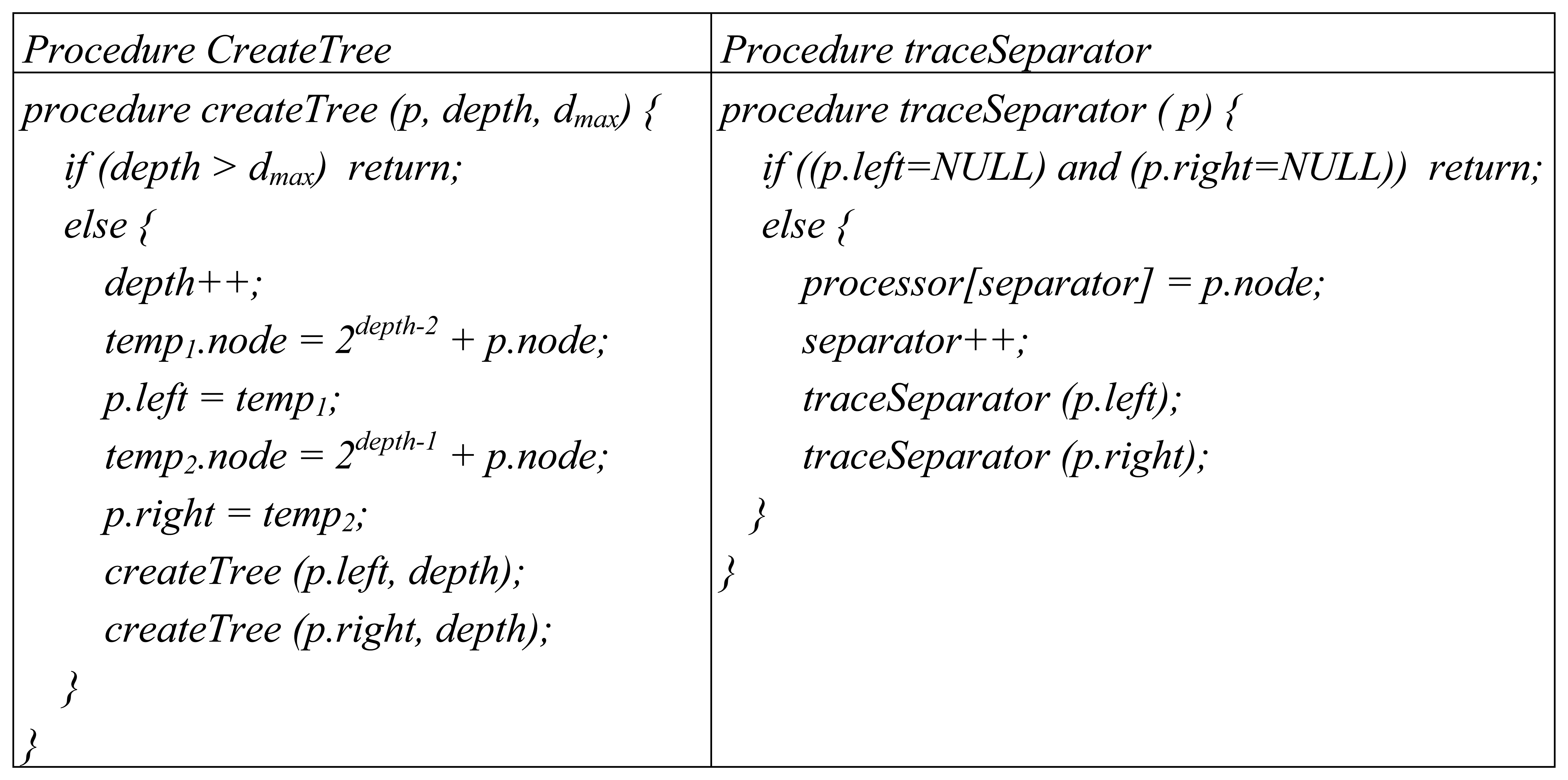
For assigning the separators, a similar strategy is followed. Each separator is assigned the processor which is either one of the two processors involved while this separator emerges and the one that has not been already assigned a separator before. To speed up the procedure, separator 1 is assigned the processor number 0, and the processor number 1 is never used while assigning separators to the processors. This algorithm, presented in Figure 21, maps the separators so that when a variable in the separator is needed it can be reached in one step of communication at most. Under such a scheme of parallelization, the number of iterations required for processing a total of p separators is reduced from O(p) to O(log p).
Procedures CreateTree and traceSeparator called in Figure 21 are listed in Figure 22 separately. These two recursive routines simply create and visit respectively a balanced binary tree whose depth first traversal corresponds exactly to the scheme used in numbering the separators as they are formed on the course of the recursive LGB algorithm.
7. Conclusions and Future Directions
In this study, a novel heuristic which performs fast was developed, and it has been shown to be superior to the method of obtaining vertex separators indirectly from edge separators. When coupled with appropriate combinatorial methods such as bipartite graph matching, it is conjectured to be the best viable heuristic that can be used in the refinement phase of multilevel nodal graph partitioning schemes. Although it is generally conjectured that problems on vertex separators are harder than the corresponding problems on edge separators [28], this study has managed to transform Kernighan-Lin heuristic, a well-known bisection algorithm on edge separators, to an easily and efficiently usable form on vertex separators.
Some difficult issues remain to be explored such as the optimality bounds for the separator size to be investigated, and modification and testing of LGB in different problem domains. Another area of future research is the investigation of the intrinsic characteristics of line graphs which would lead to the development of more efficient heuristic algorithms. A thorough experimental evaluation of the algorithm with respect to different types of randomly generated graphs is considered to be of great value in that respect. Another further improvement on LGB may be to apply a look-ahead type of bin search so that insertion to the bins may also take into account another criterion so as to favor nodes with more number of edges labeled the same. This is expected to help enhance the elasticity of the moves such that more number of nodes (due to connectivity) will have the capability to move freely.
Acknowledgments
The author would like to thank anonymous referees for their careful reading.
References and Notes
- Dellnitz, M.; Junge, O.; Koon, S.W.; Lekien, F.; Lo, M.W.; Marsden, J.E.; Padberg, K.; Preis, R.; Ross, S.D.; Thiere, B. Transport in dynamical astronomy and multibody problems. International Journal of Bifurcation and Chaos 2005, 15, 699–727. [Google Scholar]
- Diekmann, R.; Dralle, U.; Neugebauer, F.; Römke, T. PadFEM: a portable parallel FEM-tool. Proceedings of High Performance Computing and Networking 1996, 580–585. [Google Scholar]
- Berti, G.; Träff, J.L. What MPI could (and cannot) do for mesh-partitioning on non-homogeneous networks. Proceedings of PVM/MPI 2006, 293–302. [Google Scholar]
- Wheat, S.R.; Devine, K.D.; Maccabe, A.B. Experience with automatic, dynamic load balancing and adaptive finite element computation. Proceedings of the 27th Hawaii International Conference on System Sciences 1994, 463–472. [Google Scholar]
- Nakajima, K. Solid earth simulation using GeoFEM platform on the earth simulator. Proc. SIAM Conference on Computational Science & Engineering 2003. [Google Scholar]
- Burchard, H.; Deleersnijder, E.; Meister, A. Application of modified Patankar schemes to stiff biogeochemical models for the water column. Ocean Dynamics 2005, 55, 326–337. [Google Scholar]
- Frese, U.; Schroder, L. Closing a million-landmarks loop. Proc. IEEE/RSJ International Conference on Intelligent Robots and Systems 2006, 5032–5039. [Google Scholar]
- Krauthausen, P.; Kipp, A.; Dellaert, F. Exploiting locality in SLAM by nested dissection. Proc. Robotics: Science and Systems Conference 2006. [Google Scholar]
- Kernighan, B.W.; Lin, S. An efficient heuristic procedure for partitioning graphs. Bell System Technical Journal 1970, 49, 291–307. [Google Scholar]
- Gupta, A. Fast and effective algorithms for graph partitioning and sparse-matrix ordering. IBM Journal of Research 1997, 41, 171–183. [Google Scholar]
- Fiduccia, C.M.; Mattheyses, R.M. A linear-time heuristic for improving network partition. Proceedings of the 19th Design Automation Conference 1982, 175–181. [Google Scholar]
- Duff, I.S.; Erisman, A.M.; Reid, J.K. Direct Methods for Sparse Matrices; Oxford University Press: New York, 1987. [Google Scholar]
- George, J.A.; Liu, J.W.H. An automatic nested dissection algorithm for irregular finite element problems. SIAM Journal on Numerical Analysis 1978, 15, 1053–1069. [Google Scholar]
- George, J.A.; Liu, J.W.H. The evolution of the minimum degree ordering algorithm. SIAM Review 1989, 31, 1–19. [Google Scholar]
- Gilbert, J.R.; Tarjan, R.E. The analysis of a nested dissection algorithm. Numerische Mathematik 1986, 50, 377–404. [Google Scholar]
- Liu, J.W.H. A graph partitioning algorithm by node separators. ACM Transactions on Mathematical Software 1989, 15, 198–219. [Google Scholar]
- Selvakkumaran, N.; Karypis, G. Multi-objective hypergraph partitioning algorithms for cut and maximum subdomain degree minimization. Proc. IEEE/ACM International Conference on Computer Aided Design 2003, 726–733. [Google Scholar]
- Driessche, R.V.; Roose, D. Dynamic load balancing with a spectral bisection algorithm for the constrained graph partitioning problem. Proceedings of the International Conference and Exhibition on High Performance Computing and Networking 1995, 392–397. [Google Scholar]
- Bui, T.N.; Jones, C. Finding good approximate vertex and edge partitions is NP-hard. Information Processing Letters 1992, 42, 153–159. [Google Scholar]
- Skiena, S. Implementing Discrete Mathematics: Combinatorics and Graph Theory with Mathematica; Addison-Wesley: Reading, MA, 1990; pp. 135–139. [Google Scholar]
- Liu, J.W.H.; Ashcraft, C. Using domain decomposition to find graph bisectors. BIT Numerical Mathematics 1997, 37, 506–534. [Google Scholar]
- Pothen, A.; Simon, H.; Liou, K.P. Partitioning sparse matrices with eigenvectors of graphs. SIAM Journal on Matrix Analysis and Applications 1990, 11, 430–452. [Google Scholar]
- Lipton, R.J.; Tarjan, R.E. Applications of a planar separator theorem. SIAM Journal on Computing 1980, 9, 615–627. [Google Scholar]
- Hendrickson, B.; Rothberg, E. Effective sparse matrix ordering: just around the BEND. Proceedings of 8th SIAM Conference on Parallel Processing for Scientific Computing 1997. [Google Scholar]
- Pothen, A. Graph partitioning algorithms with applications to scientific computing. In Parallel Numerical Algorithms; Keyes, D.E., Sameh, A.H., Venkatakrishnan, V., Eds.; Kluwer Academic Press, 1996. [Google Scholar]
- Karypis, G.; Kumar, V. A fast and high quality multilevel scheme for partitioning irregular graphs. SIAM Journal on Scientific Computing 1998, 20, 359–392. [Google Scholar]
- Bowen, J.P. Hypercubes. Practical Computing 1982, 5, 97–99. [Google Scholar]
- Feige, U.; Mahdian, M. Finding small balanced separators. Proceedings of the 38th annual ACM Symposium on Theory of Computing 2006, 375–384. [Google Scholar]
Figure 1.
A graph and its corresponding line graph.
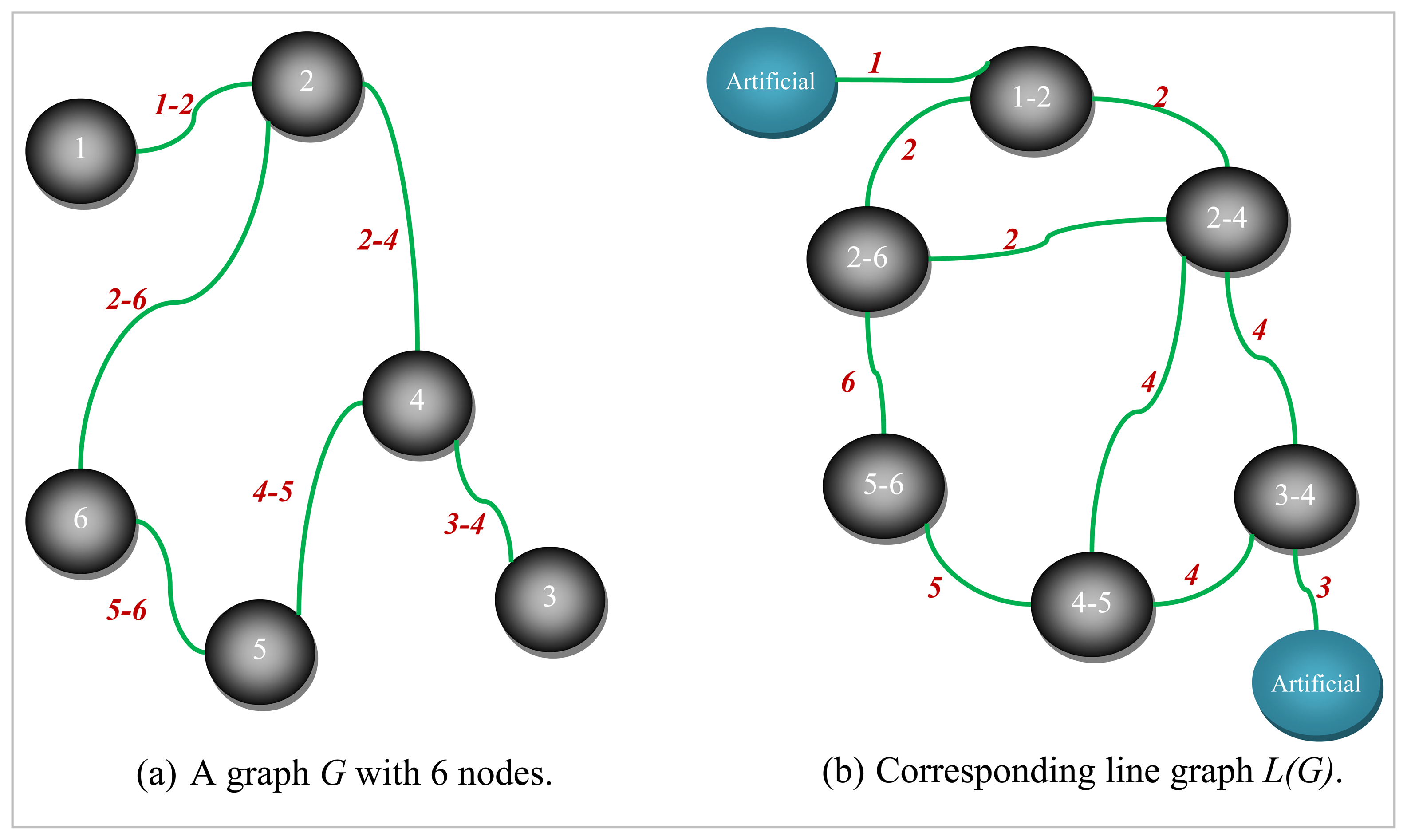
Figure 2.
An example initial partition for KLB algorithm.

Figure 3.
An example move by KLB.
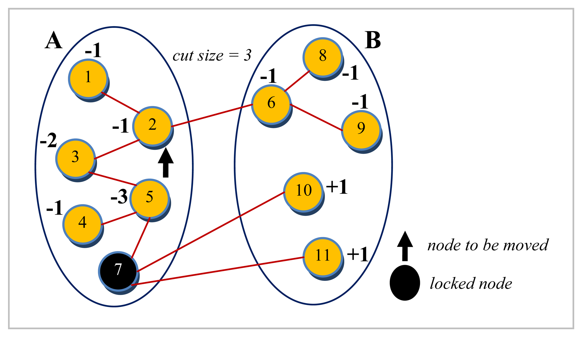
Figure 4.
Moves performed by KLB.

Figure 5.
Original graph G.
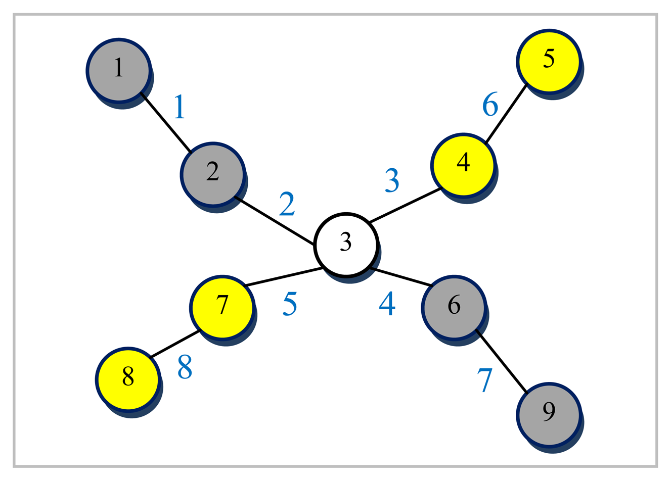
Figure 6.
Example line graph L(G) of G.

Figure 7.
Computing vertex separators.

Figure 8.
LGB Algorithm.

Figure 9.
Record structure for nodes in L(G).

Figure 10.
Bin data structures.

Figure 11.
Visualizing the edges emanating from a node in L(G).

Figure 12.
Initial gain calculations.
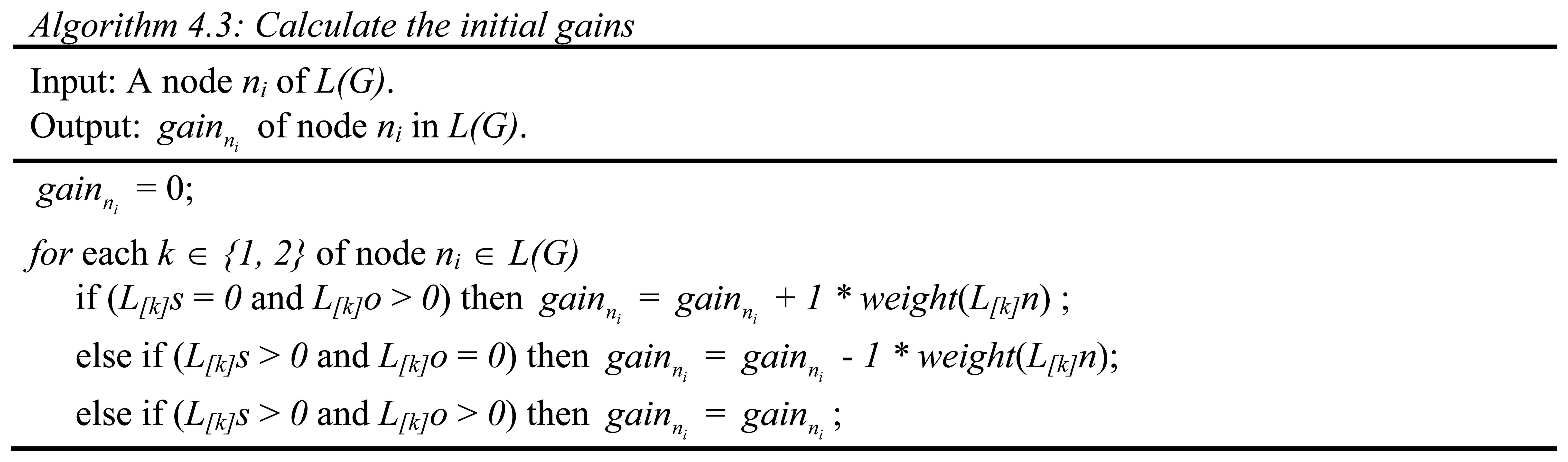
Figure 13.
Updating partition weights.
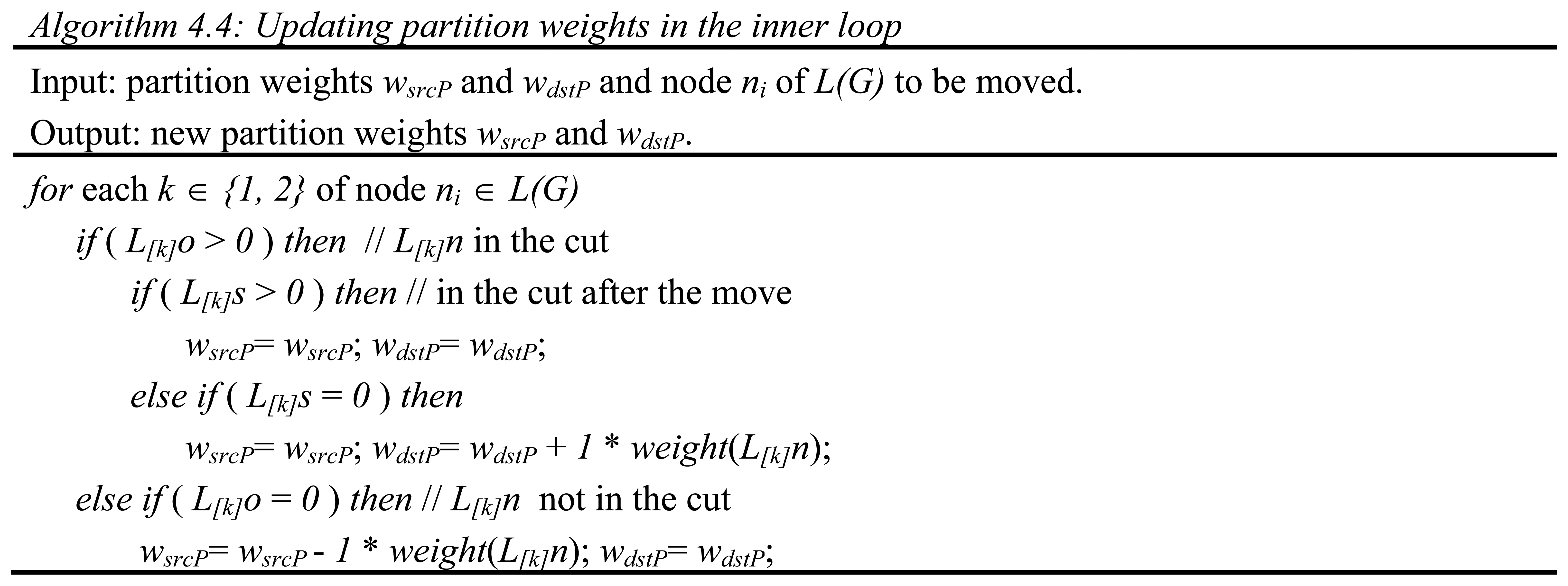
Figure 14.
Update of gain values when in different partitions.
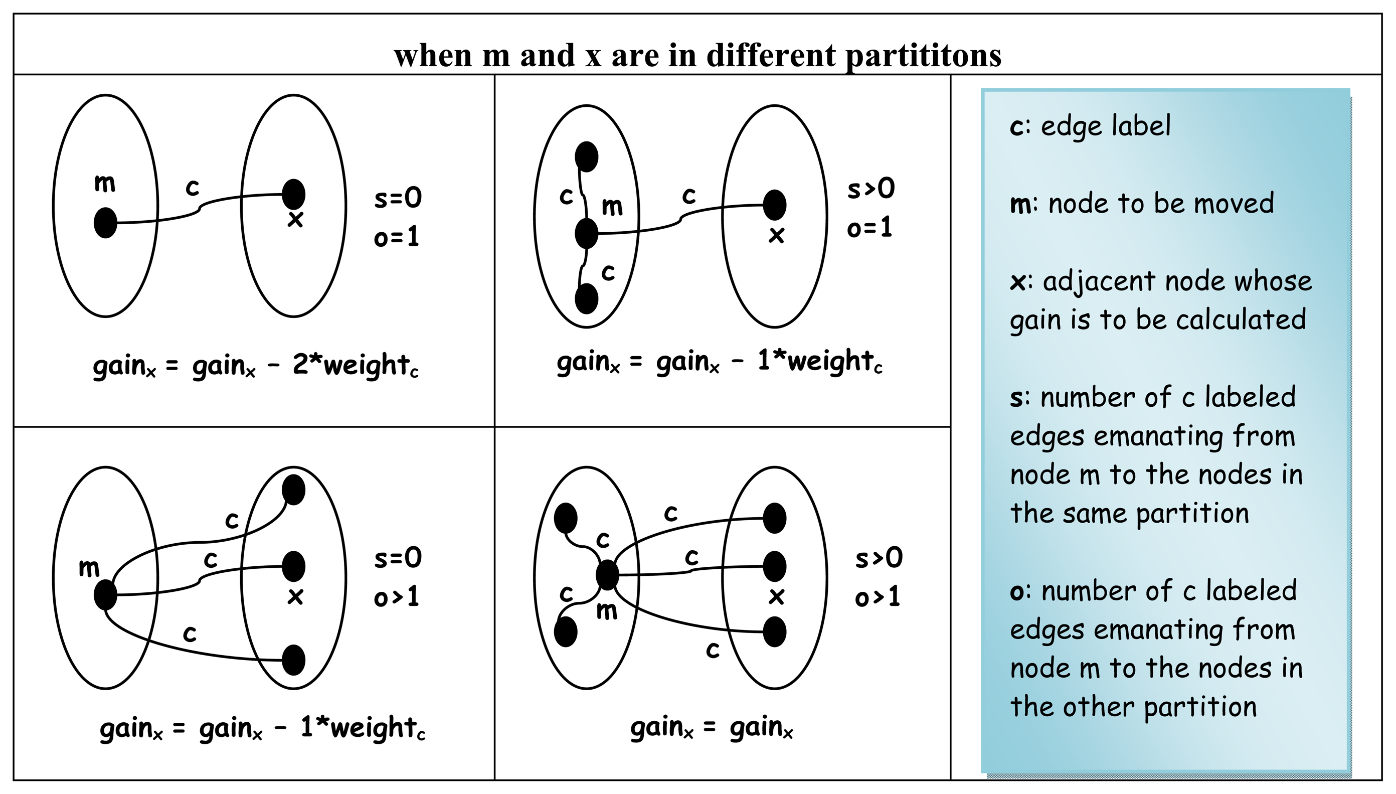
Figure 15.
Update of gain values when in the same partition.
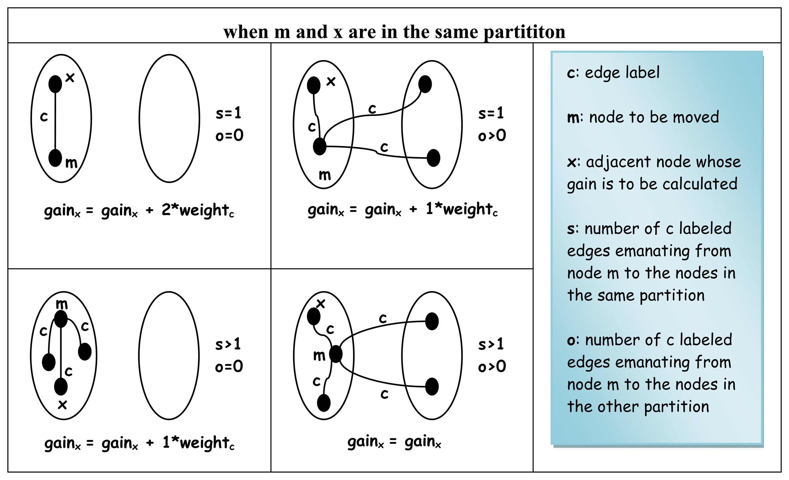
Figure 16.
Algorithm for updating the gains of adjacent nodes after a move.
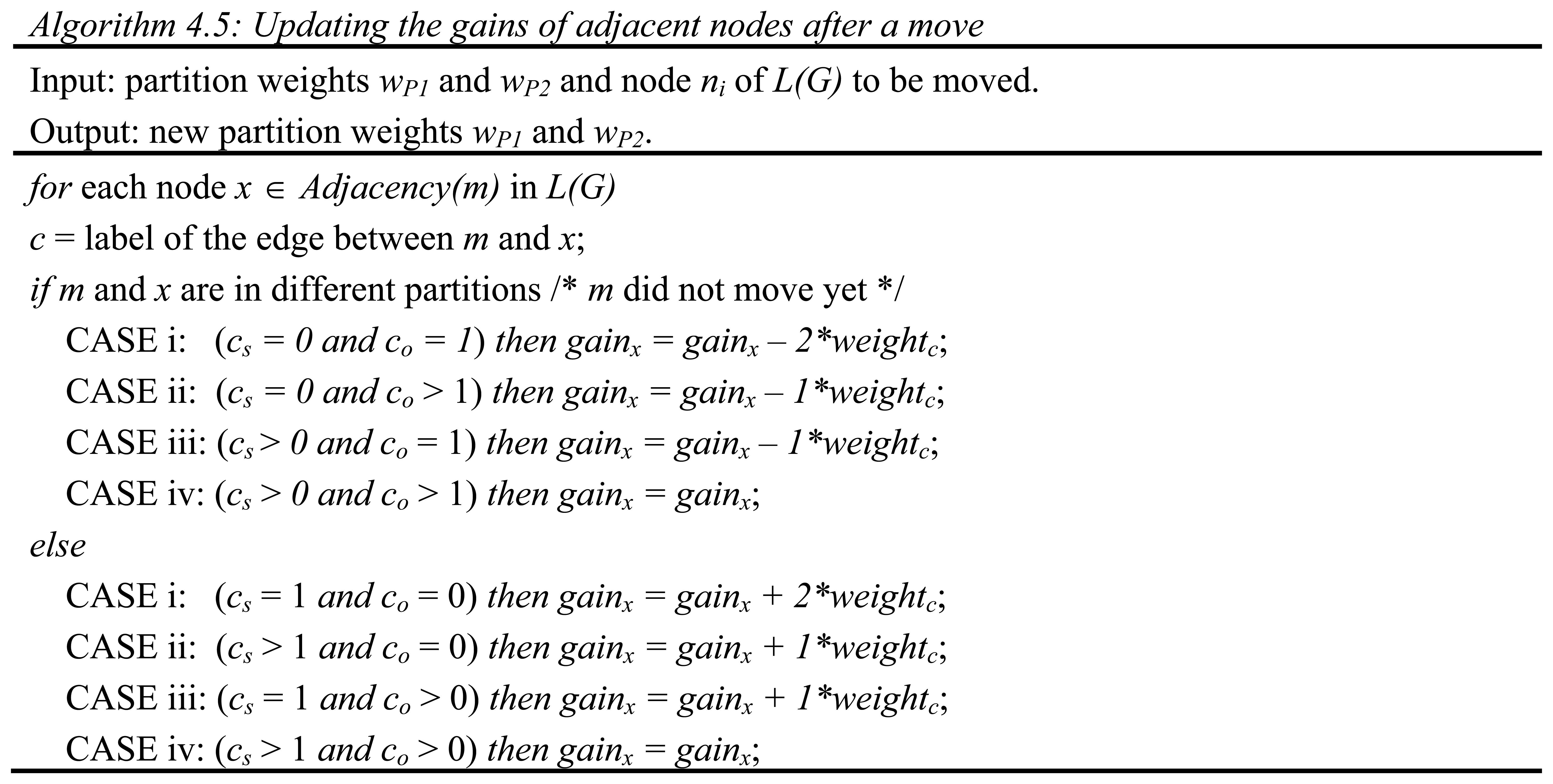
Figure 17.
A graph for comparing KLB and LGB.
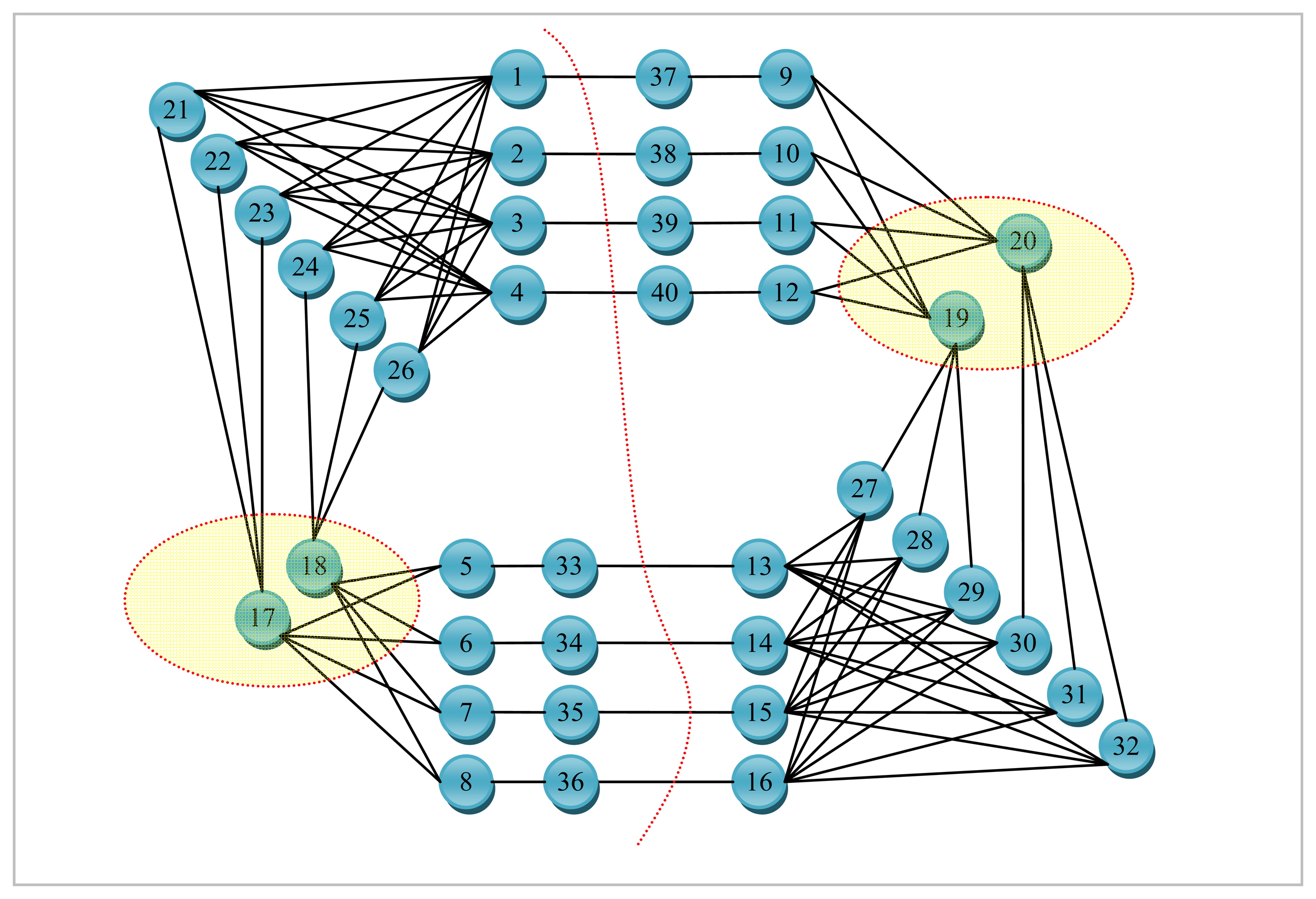
Figure 18.
A configuration where bipartite graph matching gets stuck at a local minimum.
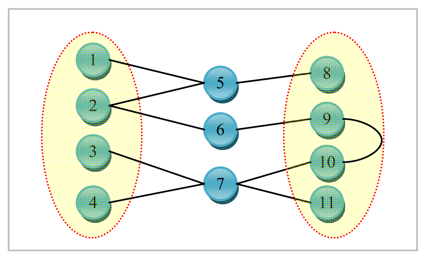
Figure 19.
Recursive LGB.
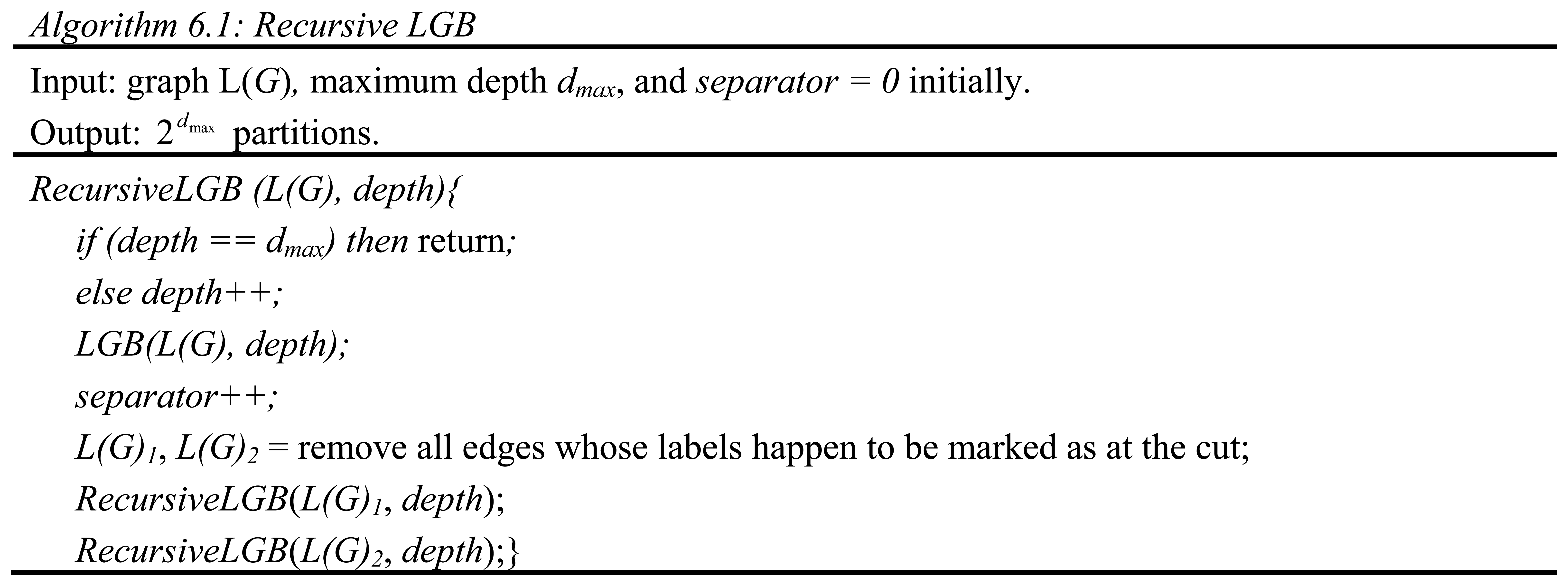
Figure 20.
Mapping partitions to processors.
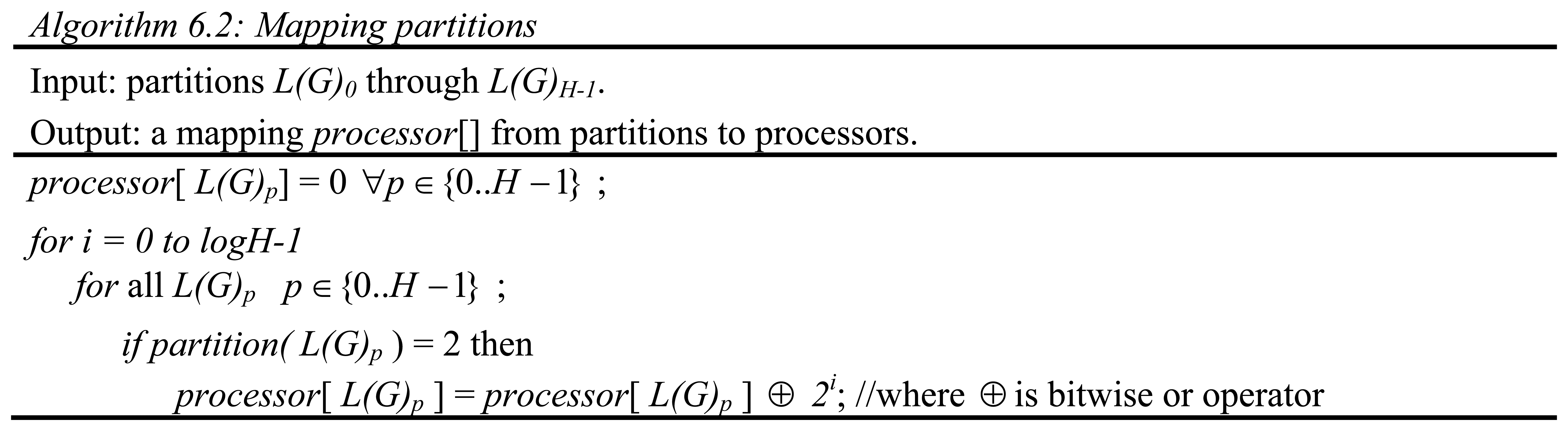
Figure 21.
Algorithm to map separators.

Figure 22.
Procedures used in mapping separators.
© 2008 by MDPI Reproduction is permitted for noncommercial purposes.
Share and Cite
MDPI and ACS Style
Evrendilek, C. Vertex Separators for Partitioning a Graph. Sensors 2008, 8, 635-657. https://doi.org/10.3390/s8020635
AMA Style
Evrendilek C. Vertex Separators for Partitioning a Graph. Sensors. 2008; 8(2):635-657. https://doi.org/10.3390/s8020635
Chicago/Turabian StyleEvrendilek, Cem. 2008. "Vertex Separators for Partitioning a Graph" Sensors 8, no. 2: 635-657. https://doi.org/10.3390/s8020635