Monitoring and Predicting Land-use Changes and the Hydrology of the Urbanized Paochiao Watershed in Taiwan Using Remote Sensing Data, Urban Growth Models and a Hydrological Model

Abstract

Monitoring and simulating urban sprawl and its effects on land-use patterns and hydrological processes in urbanized watersheds are essential in land-use and water-resource planning and management. This study applies a novel framework to the urban growth model Slope, Land use, Excluded land, Urban extent, Transportation, and Hillshading (SLEUTH) and land-use change with the Conversion of Land use and its Effects (CLUE-s) model using historical SPOT images to predict urban sprawl in the Paochiao watershed in Taipei County, Taiwan. The historical and predicted land-use data was input into Patch Analyst to obtain landscape metrics. This data was also input to the Generalized Watershed Loading Function (GWLF) model to analyze the effects of future urban sprawl on the land-use patterns and watershed hydrology. The landscape metrics of the historical SPOT images show that land-use patterns changed between 1990–2000. The SLEUTH model accurately simulated historical land-use patterns and urban sprawl in the Paochiao watershed, and simulated future clustered land-use patterns (2001–2025). The CLUE-s model also simulated land-use patterns for the same period and yielded historical trends in the metrics of land-use patterns. The land-use patterns predicted by the SLEUTH and CLUE-s models show the significant impact urban sprawl will have on land-use patterns in the Paochiao watershed. The historical and predicted land-use patterns in the watershed tended to fragment, had regular shapes and interspersion patterns, but were relatively less isolated in 2001–2025 and less interspersed from 2005–2025 compared with land-use pattern in 1990. During the study, the variability and magnitude of hydrological components based on the historical and predicted land-use patterns were cumulatively affected by urban sprawl in the watershed; specifically, surface runoff increased significantly by 22.0% and baseflow decreased by 18.0% during 1990–2025. The proposed approach is an effective means of enhancing land-use monitoring and management of urbanized watersheds.

1. Introduction

Understanding how land-use changes are associated with growth demands and the desire to preserve natural resources is critical to building livable [1] and sustainable environments. When land-use change occurs due to urbanization (building up and paving over undeveloped areas) along a city boundary, urban sprawl increases [2]. Moreover, urban sprawl is a special land-use change [2] which must be monitored and predicted to preserve natural resources in urbanized areas. Therefore, effectively monitoring and simulating urban sprawl and its effects on land-use patterns and hydrological processes in an urbanized watershed are essential to effective land-use and water resource planning and management. Remote sensing provides spatially consistent data sets for large areas with both high spatial detail and temporal frequency [3]. Moreover, remote sensing techniques have already shown their value in mapping urban areas, and as data sources for analyzing and modeling urban growth and land-use change [3-6] and hydrology. Thus, an integrated approach coupled with urban sprawl and hydrological modeling using remote sensing data that simulates and assess land-use changes, land-use patterns and their effects on hydrological processes at the watershed level is crucial to land-use and water resource planning and management in an urbanized watershed.

A thorough understanding of land-use dynamics is necessary for reconstructing past land-use/land cover changes and for predicting future changes, and, thus, may elucidate sustainable management practices aimed at preserving essential landscape functions [7, 8] and natural resources. Land-use change models have been developed to delineate land-use driving factors that influence land-use changes, and precisely predict land-use change patterns and variations in space and time. Different land-use change models, such as stochastic models, optimization models, dynamic process-based simulation models and empirical models, have been used to explore land-use changes [9]. The SLEUTH model is a bottom-up computational simulation model that uses adaptive cellular automata to simulate the manner in which cities grow and change their surrounding land [10]. Another model is the CLUE-s model, which is a top-down model that simulates land-use change using empirical quantified relationships between land use and its driving factors in combination with dynamic modeling [11]. Both models have been successful applied in many land-use change modeling cases [1, 8, 10-21].

When land-use change resulting in land-use/cover pattern changes is assessed, composition, configuration, and connectivity are primary descriptors of the landscape or land-use patterns [21, 22]. The composition, configuration and connectivity of land-use/cover patterns can be quantified using spatial landscape metrics that characterize and quantify land-use/cover composition and configuration [21]. Moreover, these metrics can be applied as improved representations of spatial urban characteristics and result in enhanced interpretations of modeling results [3] and remote-sensing historical land-uses. These metrics can include the number of patches, area, patch shape, total edge of patches, nearest-neighbor distance, landscape diversity, interspersion and contagion metrics in representing land-use/cover patterns, including compositions and configurations. Moreover, landscape metrics are also useful as an initial approximation of broad-level landscape patterns and processes, and for characterizing differences among planned and design alternatives, and have been recommended as an appropriate tool for land-use planning and design [21, 23, 24].

Hydrological models provide a framework for conceptualizing and investigating relationships between climate, human activities (e.g., land-use change) and water resources [25] and have been applied for quantifying the impact of land-use change on hydrologic components [26]. Therefore, hydrological models are a useful means of assessing the effects of changes in land-use patterns resulting from policy decisions, economic incentives or economic structural changes [27]. Recently hydrological simulation models have been widely used to quantify the influence of land use change on the hydrologic cycle. Hydrological simulation models have recently been widely used to quantify the influence of land-use change on hydrologic cycles. The GWLF model developed by Haith and Shoemaker [28] is a combined distributed/lumped parameter watershed model that simulates runoff, sediment, and nutrient loadings in watersheds given sources (e.g., agricultural, forested, and developed land). Surface loading is distributed in the sense that it allows multiple land use and land cover scenarios in which each area is assumed to have homogeneous attributes. Surface loading is distributed in the sense that it allows multiple land use and land cover scenarios in which each area is assumed to have homogeneous attributes when addressed by the model [28]. For subsurface loading, the model functions as a lumped parameter model utilizing a water-balance scheme. Daily water balances are derived for unsaturated and saturated sub-surface zones, in which infiltration is calculated as the difference between precipitation and snowmelt minus surface runoff plus evapotranspiration [28].

This study uses an integrated approach that combines urban sprawl, land-use, landscape metrics and hydrological models. Four historical SPOT images for 1990, 1993, 1998 and 2000 for the Paochiao watershed, Taiwan, are first classified using supervised classification with maximum likelihood and fuzzy methods. The classified land-use data for all years are input into the landscape pattern analysis package Patch Analyst in GIS software Arcview 3.0 a; data are also input into the SLEUTH model and CLUE-s model. The SLEUTH model predicted land-use demands and simulate land-use changes from 2001–2025 for the Paochiao watershed. Patch Analyst calculates landscape metrics for historical land-use and simulated land-use patterns at a landscape level to analyze urban sprawl impact on land-use patterns. Finally, the hydrological components, which are based on simulated land-uses, are simulated using the GWLF model to predict and assess urban sprawl impact on watershed hydrology.

2. Methods and Materials

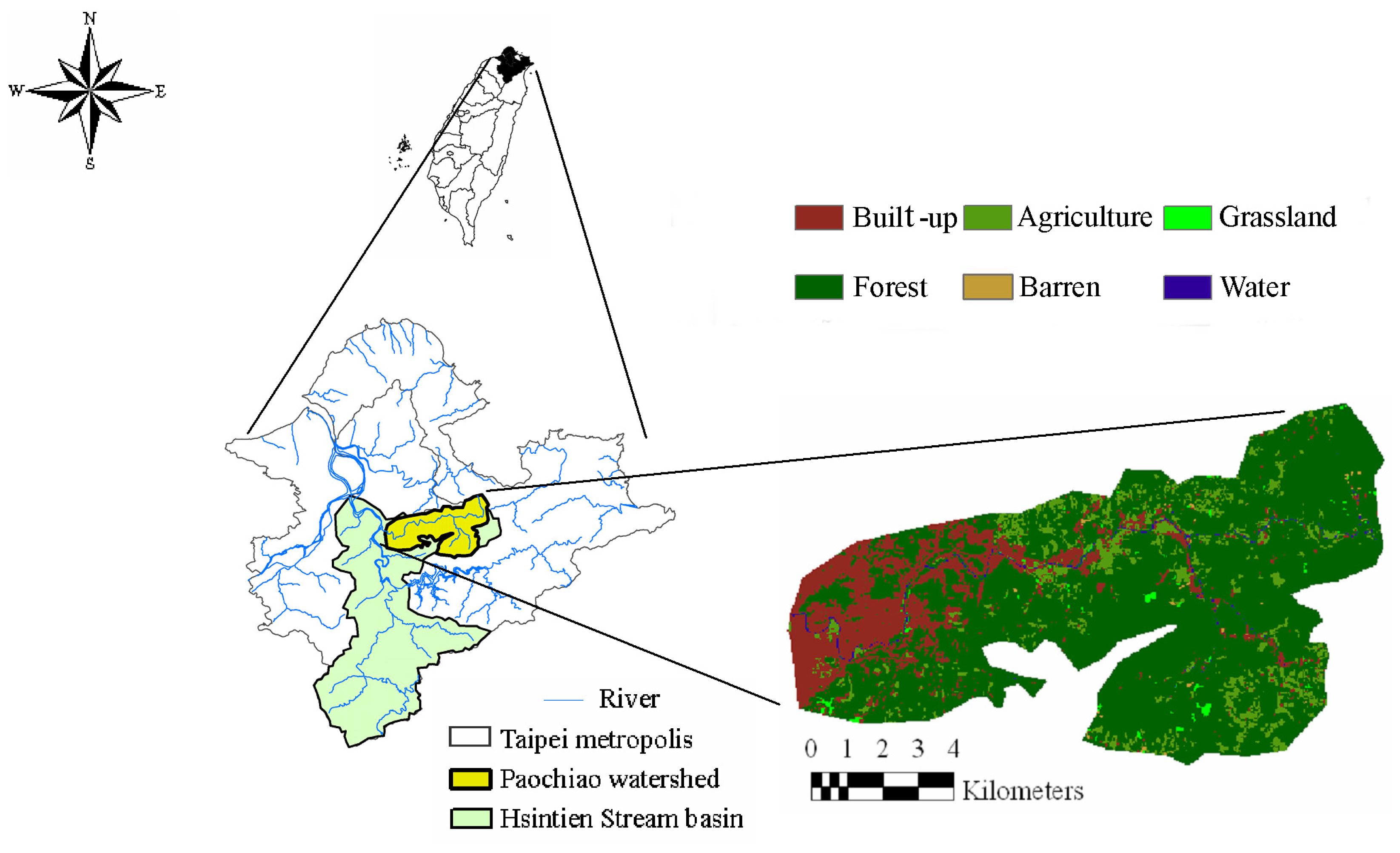
2.1. Study watershed and data

The Paochiao watershed is an urbanized watershed in the Tamsui River Basin. The watershed is bordered to the south by the Taipei metropolitan area (Figure 1). The Paochiao watershed is approximately 98.61 km² with a mean elevation of 214.82m. Due to the expansion of the Taipei metropolitan area, land use and its patterns in the Paochiao watershed have changed over the last decade. Under an increasing population, the watershed has become a high-density urbanized watershed, especially in the downstream watershed area. Total population in 2000 was 237,861. The land uses in 2000 were 74.78%, 15.26%, 8.24%, 0.83%, 0.65 %, and 0.24% for forest, built-up land, cultivated land, grassland, water, and bare land, respectively.

2.2. Land-use images and classification

Four SPOT images were purchased from the space and remote-sensing research center in Taiwan, and were selected for watershed land-use classification on March 27, 1990, December 25, 1993, July 16, 1998, and January 2, 2000. Supervised classification and fuzzy convolution are performed using the software ERDAS IMAGINE with 1/5000 black and white aerial photographs. The forest, built-up land, cultivated land, grassland, water, and, bare land classes were marked on the 1/5000 aerial photographs by the Aerial Survey Office, Forestry Bureau in Taiwan. Next, the classified images and geographical data (roads, buildings, slopes and band ranges) of the study watershed formed the knowledge base in the Knowledge Engineer of IMAGINE for final classifications of SPOT images. The IMAGINE user manual provided details of theorems of these effective classification methods. Moreover, kappa values were calculated for the final classification accuracy assessment. Land uses were classified into the following six categories: forest; built-up land; cultivated land; grassland; water; and, bare land (Figure 2). In total, 300 pixels were used in assessing classification accuracy, and each training class had 10–134 pixels. The total accuracy and kappa values were 90% and 0.86, 90% and 0.85, 90% and 0.86, and 89% and 0.84 for classification of images for 1990, 1993, 1998, and 2000, respectively. Land-use classes of forest, built-up land, cultivated land and Grassland had high classification accuracies (92%∼96%, 85%∼96%, 73%∼90% and 63%∼90%), while class bare land had low classification accuracies (42%∼60%) in the classifications.

2.3. SLEUTH model

The SLEUTH model combined urban growth and the land-cover change model developed by Clarke [29], which is a probabilistic model that uses Monte Carlo routines to generate multiple simulations of growth. As a cellular automata model, space is represented as a regular grid of cells that change states as the model iterates. State changes are controlled by a set of conceptually simple rules that specify neighborhood conditions, such as slope suitability, that must be met before a change can occur [30]. For this model, transition rules between time periods are uniform across space, and are applied in a nested set of loops [10]. The outermost of the loops executes each growth period, whereas an inner loop executes growth rules for a single year. The transition rules implemented involve randomly choosing a cell and investigating the spatial properties of that cell's neighborhood, and then urbanizing the cell based on probabilities influenced by other local characteristics [29]. Within the urban growth module, urban dynamics are simulated using four growth rules [30]:

• Spontaneous new growth, which simulates random urbanization of land.
• New spreading centers, which simulate development of new urban centers.
• Edge growth, which represents the outward spread of existing urban centers.
• Road-influenced growth, which simulates the influence of the transportation network on development patterns.

The SLEUTH model is calibrated to simulate urban development patterns over a given time period, and then forecasts these patterns into the future under a set of exclusion layers that represent land use [30]. During calibration, each simulation is compared with control years within the time series, and averaged fit statistics are produced to measure the performance of a set of coefficient values in reproducing observed urban development patterns [30]. Calibration of the SLEUTH model produces a set of five parameters or coefficients (Diffusion, Breed Coefficient, Spread Coefficient and Road Gravity Factor) that describe individual growth characteristics, and that, when combined with other characteristics, can describe several different growth processes. During the calibration phase, 13 parameters have been proposed to determine the goodness-of-fit of simulated results to the known data [10], six of those matrices were adopted in this study to analyze modeling performance (

Table 1. Statistical matrices of fitting goodness for SLEUTH modeling (after [10, 16]).

Statistical matrices	Description
Compare	Ratio of modeled population (PM) of urban pixels to the observed population of urban pixels (PO) for the final control year: Compare = PM(final year)/PO(final year). If PM>PO, then Compare =1 − PM(final year)/ PO(final year).
Population	Least squares regression score for modeled urban pixels compared with actual urban pixels for each control year.
Edges	Least squares regression score for modeled urban edge count compared to actual urban edge count for the control years
Clusters	Least squares regression score for modeled urban clustering compared to known urban clustering for the control years
Lee-Sallee	Ratio of the intersection to the union of the simulated (SMi) and the actual (SOi) urban areas for each control year (i) averaged over all control years (N):$\text{Lee}-\text{Salee}=\frac{\sum (S_{\mathit{\text{Mi}}}\cap S_{\mathit{\text{Oi}}})/(S_{\mathit{\text{Mi}}}\cup S_{\mathit{\text{Oi}}})}{N}$
F-Match	Ratio of the number of pixels categorized into correct land-use (C) to the sum of the number of pixels categorized into correct land-use (C) and wrong land-use (W): F-Match = ∑(C)/(C + W)

). All matrices have values of 0–1, with 1 indicating a perfect fit.

In this study, input images for SLEUTH modeling are four historical images of land use for 1990, 1993, 1998, and 2000, transportation networks in 1990 and 2000, and 40×40 m² digital elevation models (DEMs) for determining hillsides and slopes, while the excluded land-use class in SLEUTH modeling is the land-use class of water

2.4. CLUE-s model

In the CLUE-s model, the non-spatial module calculates the area of change for all land-use types at an aggregate level, and the spatial module in CLUE-s translates demands into land-use changes at various locations within the study region [31]. The relationships between land use and its drivers can be fitted using stepwise logistic regression. Moreover, probability maps for all land uses can be established using logistic regression models. The explicit spatial allocation procedure converts non-spatial demands into land-use changes at various locations in the study area. The relationships between land uses and their drivers were evaluated by the following stepwise logistic regression [31]:

$$\mathit{\text{Log}}(\frac{P_i}{1-P_i})={\beta }_0+{\beta }_1{X}_{1,i}+{\beta }_2{X}_{2,i}+\cdots +{\beta }_n{X}_{n,i}$$

(1)

where Pi is the probability of a grid cell for the occurrence of a considered land use type, the Xs are driving factors, and β_i is the coefficient of each driving factor in the logistic model.

After fitting the logistic regression models to all land uses, the restricted area and land-use transition rules were specified for the study watershed. Finally, land-use change is allocated in the following iterative procedure based on probability maps, decision rules are combined with actual land-use maps and demand for different land uses [31]. The first step in the iterative procedure generates a preliminary allocation for which the iteration variable has an equal value for all land-use types by allocating the land-use type with the highest total probability of land use occurrence for the considered grid cell [31]. Conversions not permitted in the conversion matrix are not allocated. Total allocated area for each land use is then compared to land use demand. For land use types for which the allocated area is smaller than the demand area, the value of the iteration variable is increased. For land use types with excessive allocation, the value of the iterative variable is decreased. These procedures are repeated as long as demands are incorrectly allocated. When allocation and demand are equal, the final land use at this time step is saved and the allocation procedure continues for the next year until the target year is reached. Moreover, grid cells in the restricted area cannot be converted into other land uses during the allocation procedure.

In this study, land use demands in the CLUE-s model were set according to simulation results obtained by the SLEUTH model for 2001–2025. The area of the water body was assumed constant during the simulation periods. An area with a slope > 21% was defined as restricted areas. Land-use transition rules indicate that forested, cultivated land, grassland, and bare land can be converted between any of these land-use classes and built-up land, while the water body remains unchanged. Built-up land can be converted into other land uses with the highest conversion costs. The driving factors of land-use transition in this study are distance to major roads, altitude, slope, the distance to river, the distance to built-up land, distance to urban planning areas, soil drainage, soil erosion coefficient, and population density.

2.5. Landscape Metrics

To assess changes to land-use patterns, landscape metrics are calculated using Patch Analyst [32] in GIS software ArcView 3.2a. Seven landscape indices—Number of Patches (NP), Mean Patch Size (MPS), Mean Shape Index (MSI), Area Weight Mean Shape Index (AWMSI), Total Edge (TE), Mean Patch Fractal Dimension (MPFD), Mean Nearest Neighbor (MNN) and Interspersion and Juxtaposition Index (IJI) were used to present land-use composition and configuration at the landscape level in the watershed.

The adopted matrices are calculated as follows.

$$\text{NP}=n_i,$$

(2)

where n_i is the number of patches of land-use class i.

$$\text{MPS}=\frac{1}{n_i}\sum _{j=1}^{n_i}{a}_{\mathit{\text{ij}}},$$

(3)

where a_ij is the j^th patch area (m²) of land-use class i.

$$\text{MSI}=\frac{\sum _{j=1}^{n_i}\frac{0.25p_{\mathit{\text{ij}}}}{\sqrt{a_{\mathit{\text{ij}}}}}}{n_i},$$

(4)

where p_ij is the j^th patch perimeter (m) of land-use class i.

$$\text{AWMSI}=\sum _{j=1}^{n_i}\frac{0.25p_{\mathit{\text{ij}}}}{\sqrt{a_{\mathit{\text{ij}}}}}\frac{a_{\mathit{\text{ij}}}}{\sum _{j=1}^{n_i}{a}_{\mathit{\text{ij}}}}.$$

(5)

$$\text{TE}=\sum _{k=1}^m{e}_{\mathit{\text{ik}}},$$

(6)

where m is the total number of patch classes presented, e_ik is the total length (m) of the edge between patch classes i and k.

$$\text{MPFD}=\frac{\sum _{j=1}^{n_i}\frac{2ln(0.25p_{\mathit{\text{ij}}})}{ln{a}_{\mathit{\text{ij}}}}}{n_i}$$

(7)

$$\text{MNN}=\frac{\sum _{j=1}^{n_i}{h}_{\mathit{\text{ij}}}}{n_i},$$

(8)

where h_ij is the distance (m) from the j^th patch to the nearest neighboring patch of the same class, i, based on edge-to-edge distance.

$$\text{IJI}=\frac{-\sum _{k=1}^m\frac{e_{\mathit{\text{ik}}}}{\sum _{k=1}^m{e}_{\mathit{\text{ik}}}}ln\left(\frac{e_{\mathit{\text{ik}}}}{\sum _{k=1}^m{e}_{\mathit{\text{ik}}}}\right)}{ln(m-1)}(100),$$

(9)

where A is total landscape area (m²), NP is the total number of patches in the landscape, P_ij is perimeter length (m) of patch ij, a_ij is the area (m²) of patch ij, P_i is the proportion of the landscape occupied by patch type I, m is the number of patch types in the landscape, and n is the number of patches of each type in the landscape.

The MPS is used to measure patch size at the landscape and class levels. The MSI is a measure of average patch shape, or average perimeter-to-area ratio, for a particular patch type or for all patches in a landscape and classes. The MSI equals 1 when all patches in a landscape are square. Thus, the MSI increases without limits as patch irregularity increases. The AWMSI equals 1 when all patches of a corresponding patch type are circular (vector) or square (raster) [33]; Total edge is an absolute measure of total edge length for a particular patch type (class level) or for all patch types (landscape level) [33]. Mean Patch Fractal Dimension approaches 1 for shapes with very simple perimeters, such as circles or squares, and approaches 2 for shapes with highly convoluted, plane-filling perimeters [33]. At a landscape level, the MNN considers only those patches with neighboring patches. The IJI measures the degree to which patch types are interspersed (not necessarily dispersed); high values indicate that patch types are well interspersed (equally adjacent to each other), whereas low values characterize landscapes in which patch types are poorly interspersed (disproportionate distribution of patch type adjacencies) [33]. The IJI approaches 0 when the distribution of patch adjacencies among unique patch types becomes increasingly uneven. The IJI is 100 when all patch types are equally adjacent to all other patch types.

2.6. Hydrological Model

In the GWLF model, streamflow comprises surface runoff (Q_t) calculated by the Soil Conservation Service Curve Number and groundwater discharge (G_t) estimated by modeling a shallow groundwater aquifer as a linear reservoir. Storage of a shallow saturated zone is derived by the following water balance equation [28]:

$$S_{t+1}=S_t+P{C}_t-G_t-D_t$$

(10)

$$G_t=r{S}_t$$

(11)

where S_t (cm) is the water content of a shallow ground water aquifer at the start of day t, PC_t is the percolation (cm) and D_t is the deep seepage (cm) during day t, and r is the recession coefficient. Percolation proceeds when soil moisture of an unsaturated zone exceeds field capacity, and is calculated by

$$P{C}_t=max[0,U_t+I_t-E{T}_t-U^{*}]$$

(12)

where U_t is soil moisture content of a root zone (cm) at the start of day t, I_t is the infiltration (cm), ET_t is evapotranspiration (cm) during day t, and U* is the maximum soil water capacity (cm). Infiltration can be calculated by

$$I_t=R_t-Q_t$$

(13)

where R_t is rainfall. Evapotranspiration is impacted by atmospheric conditions and soil use and soil moisture content, whose relationship is

$$E{T}_t=\mathit{\text{Min}}[k_{\mathit{\text{st}}}\times k_{\mathit{\text{ct}}}\times {\mathit{\text{PET}}}_t,U_t+I_t]$$

(14)

where k_st and k_ct are coefficients of soil moisture stress and land cover, respectively, and PET_t is the potential evapotranspiration calculated using the Hamon equation (Hamon, 1961). Water content in the unsaturated zone is traced by

$$U_{t+1}=U_t+I_t-E{T}_t-P{C}_t$$

(15)

Historical and future land-use patterns were fed into the GWLF model to simulate hydrological components of the Paochiao watershed. Stream flow data was used for 1990–2003 to verify the simulated stream-flow modeled using the GWLF model (Figure 3). Additionally, the R² value of the linear regression model of the monthly mean stream of simulated and observed data was 0.90, and the difference between simulated and observed data was significant at p ≤ 0.01.

3. Results

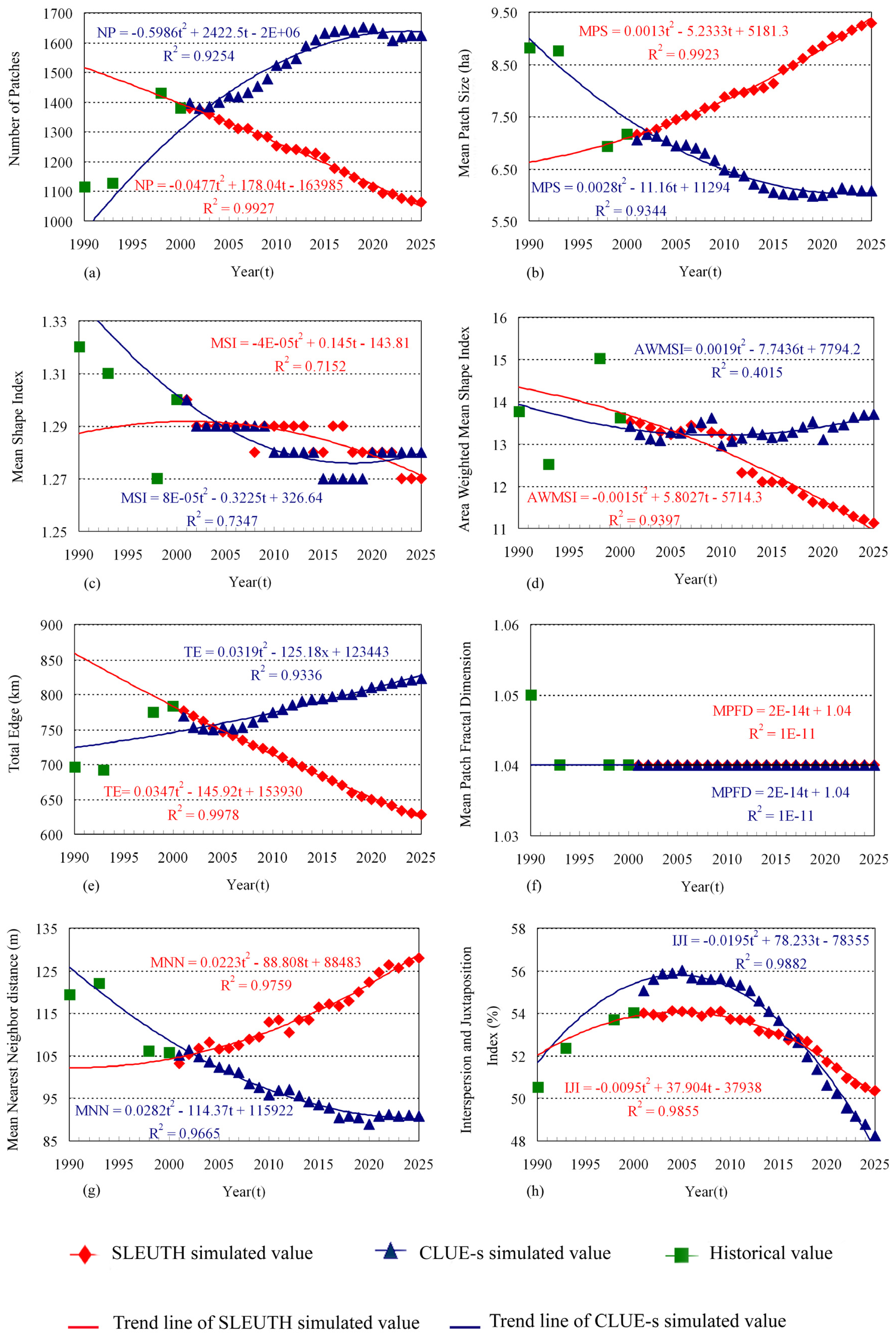
3.1. Land use change modeling

Statistical matrices of goodness-of-fit (Table 1), for SLEUTH modeling in this study were 0.94, 0.64, 0.93, 0.92, 0.71, and 0.91 for metrics of Compare, Population, Edges, Clusters, Lee-Sallee, and F-Match, respectively. The slightly low value for the Population parameter is due to the simulated numbers of urbanized grid cells in each year from 1990–2000 deviating from the observed numbers. This phenomenon indicates that the SLUETH model, which simulates urban sprawl based on regulating the state of grid cells in the vicinity of land-uses. The spread of urbanized grid cells may be scattered rather than diffusing from current urbanized centers. Simulation results predicted by SLEUTH modeling from 2001–2005 (Figure 4) indicate that the built-up land is the only land-use class that has a monotonic increase in its area from 1551.68 ha in 2001 to 2833.12 ha in 2025. Simulated land-use maps show that the most developed and frequently changed areas are located in the eastern part of (downstream area) and along the stream in the Paochiao watershed, especially in low elevation areas (Figure 4). The increase ratio for built-up area is 82.58%. Other areas of land-use classes all decreased with ratios of 49.31%, 47.92%, 42.40%, and 11.50% for cultivated land, bare land, grassland, and forest, respectively; the water body remained unchanged (Figure 5).

In the CLUE-s, the logistic regression model was used to predict probabilities for all land-use classes and measure the relationships between probabilities and driving factors (

Table 2. Logistics regression model for land-use classes.

Variable1	Forest	Built-up land	Cultivated land	Grassland	Bare land
DTransport	6.4E-04***2	N/A2	-9.0E-04***	-7.9E-02**2	-1.5E-03**
DEM	9.3E-04***	N/A	-4.5E-04*2	N/A	N/A
Slope	9.4E-02***	-2.0E-02	-6.7E-02***	-3.9E-02***	-4.1E-02***
DRiver	-1.1E-04***	N/A	4.1E-04***	4.2E-04***	N/A
DBuild	5.1E-03***	-2.8E-01***	-1.1E-03***	N/A	-8.9E-04
DZone	N/A	N/A	6.0E-05**	3.0E-04***	N/A
SDr	2.1E-01***	N/A	N/A	N/A	-1.2***
SErosin	8.0E-01***	N/A	2.1***	4.5***	4.1**
PDens	-4.0E-05***	2.0E-05	-3.6E-04***	N/A	-1.4E-03***
Constant	-1.5	6.2	-1.1	-5.2	-4.7
ROC3	0.9	1.0	0.7	0.7	0.8

^1.DTransport represents the minimum distance to major road; DEM represents the altitude; Slope represents the slope; DRiver represents the minimum distance to river; DBuild represents the minimum distance to built-up land; DZone represents the minimum distance to urban planning area; SDr represents the soil drainage; SErosin represents the soil erosion coefficient; PDens represents the population density.

^2.N/A represents not significant;

^‘*’represents p < 0.05 ;

^‘**’represents p < 0.01 ;

^‘***’represents p < 0.001

^3.ROC represents the relative operating characteristic value.

). The Relative Operating Characteristic (ROC) values for the models are 0.65–1.0, indicating that the models explain the predicted probabilities for all land use types, especially models for built-up areas and forest. Driving factors were altitude, distance to urban planning area, population density and soil erosion coefficient, each of which had a positive contribution to binary logistics models for agricultural land in the watershed. Distance to major roads, slope and distance to built-up areas negatively contributed to predicted probability for agricultural land. Factors distance to river, elevation, slope, distance to built-up area, and soil erosion contributed positively to probability for forest in the watershed. Factors distance to major roads and population density negatively impacted the occurrence of forest. The logistic regression model for predicting built-up areas had three negative coefficients for driving factors (slope, distance to built up area and soil erosion coefficient) and one small positive factor (population density). To predict probability of grassland, the fitted logistics model used two positive factors (distance to major roads, soil drainage) and five negative factors (distance to river, elevation, slope, distance to built up area and distance to urban planning area). Based on logistic regression models, the SLEUTH model predicted land-use demands, spatial policies and land-use conversion rules, while the CLUE-s model was applied to predict land-uses from 2001–2025. Figure 6 presents land-use maps for 2005, 2010, 2015, 2020 and 2025. These maps show that the most developed and frequently changed areas are located in the eastern part (downstream area) and along the stream of the Paochiao watershed, especially in areas with low elevations (Figure 6).

Based on logistic regression models, land-use demand, spatial policies and land use transition rules, the CLUE-s model was applied to predict land-use distributions for 2001–2025 (Figure 6). Land use demands for the CLUE-s model were set according to simulation results obtained by the SLEUTH model for 2000–2025. Mapping results show that the most developed and frequently changed areas are located in the eastern part of the downstream area and along the major stream of the Paochiao watershed, especially in areas with low elevations. A remarkable phenomenon of urbanization (Figures 6(a)–(c)) shows that the distribution of urbanized cells due to urban sprawl is scattered. The urbanized grid cells can induce a high probability of urbanization in nearby grid cells. Simulation results indicate that the present priorities for urbanization are forest, cultivated land, grassland, and bare land in that order. The other notable land-use conversions, sorted by occurrence frequencies from high to low, are transitions of grassland to forest, forest to cultivated land, and bare land to forest.

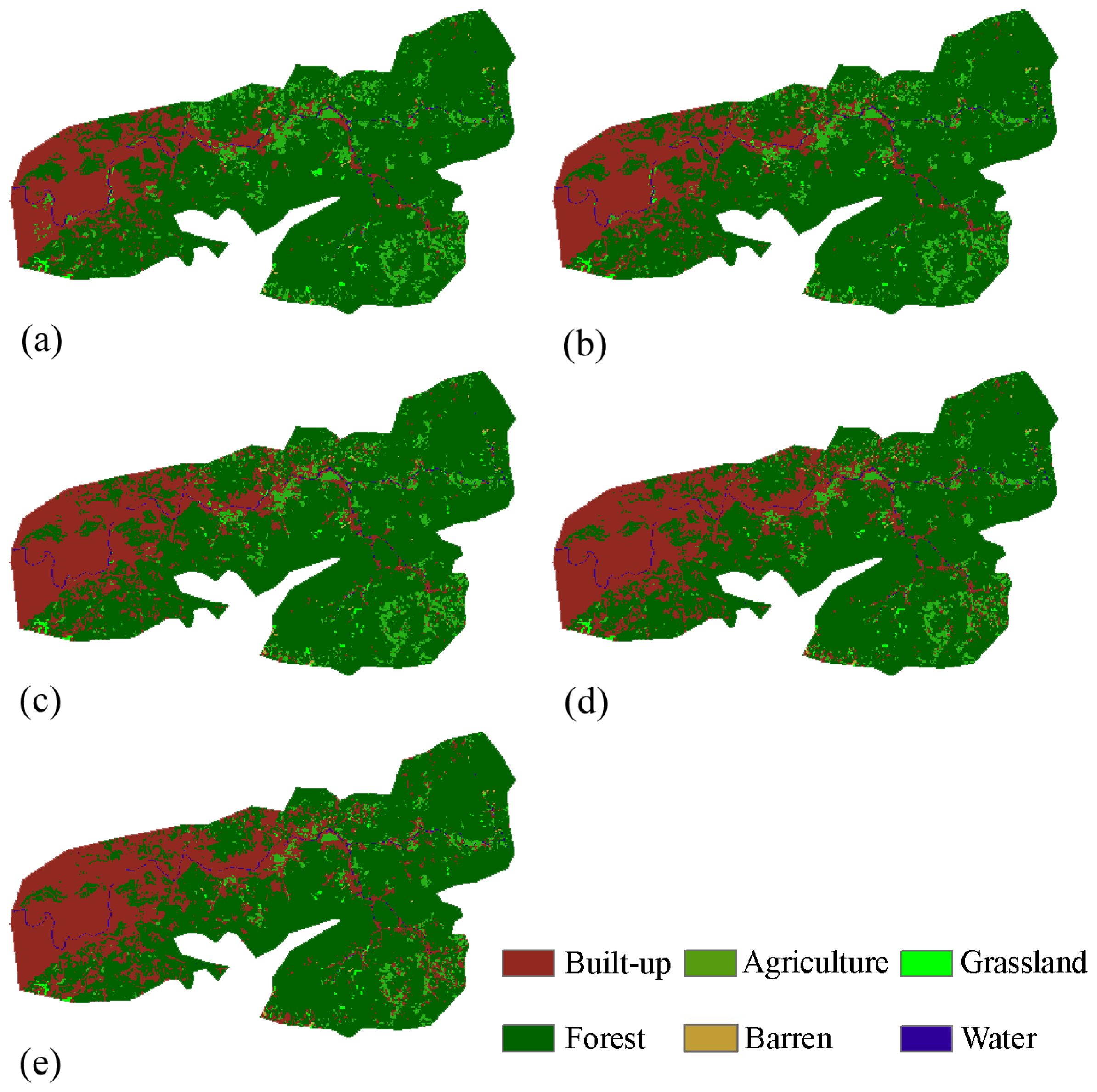
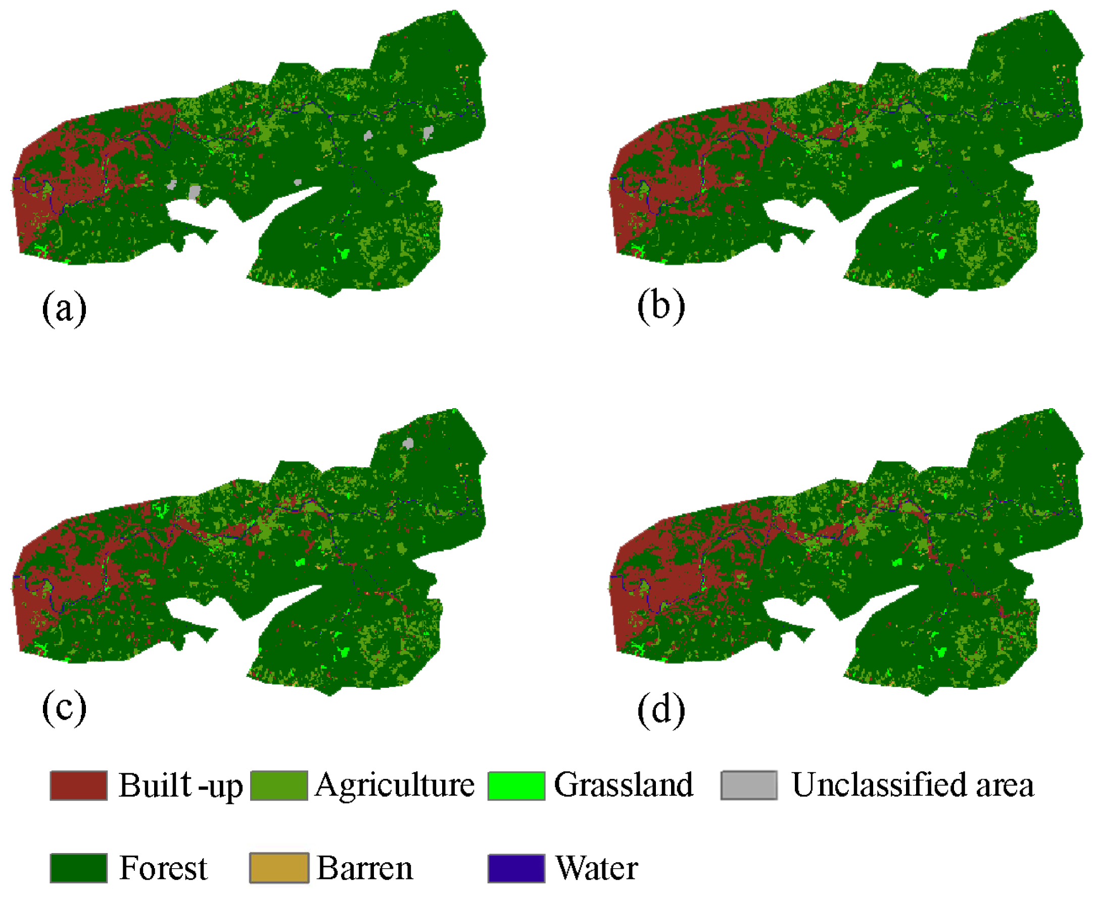
3.2. Historical and predicted land-use patterns

Figure 4 shows the predicted proportions of each land use type simulated by the SLEUTH model during simulated periods (2001–2025) in the study watershed. Figures 2, 5 and 6 show land-use changes from 1990–2025. The forested and agricultural areas decreased, however, built-up area increased from 2001 to 2025. Moreover, land uses predicted by the SLEUTH model are more clustered than those predicted by the CLUE-s model. Prediction results from both land-use model show that the built-up area expanded from the eastern part and along the stream to the mid-section of the watershed (Figures 2, 5 and 6). Figure 7 shows landscape metrics—NP, MPS, MSI, AWMSI, TE, MNN and IJI—for the patterns of historical land-use changes and simulated land-use changes predicted by the SLEUTH and CLUE-s models. Notably, NP, TE and the IJI of historical land-use increased from 1990 to 2000; MPS, MSI and MNN decreased from 1990 to 2000. The NP values of both historical and predicted land-uses simulated by the CLUE-s model increased from 1990 to 2025; however, the NP values of predicted land uses simulated by the SLEUTH model decreased from 2001 to 2025 (Figure 7(a)). The values of MPS of historical and CLUE-s predicted land-uses scenarios decreased from 1990–2025; however, the SLEUTH model predicted that land use increased from 2001–2025 (Figure 7(b)). The MSI values for all model-predicted land uses slightly decreased between 2000–2025 (Figure 7(c)). The AWMSI values of CLUE-s-predicted land uses remained constant; however, the AWMSI values of SLEUTH-predicted land uses decreases from 2001–2025 (Figure 7(d)). The TE values of historical and CLUE-s predicted land uses increased during 1990–2000 and the simulated period 2001–2025 (Figure 7(e)). The SLEUTH-predicted land uses decreased during the simulation period. The MPFD values of historical and predicted land uses remained constant, except for land use in 1990 (Figure 7(f)). Although the MNN values of historical land uses and CLUE-s-predicted land uses decreased from 1990–2025, SLEUTH-predicted land-uses increases from 2001–2025 (Figure 7(g)). The IJI values of historical land uses increased from 1990–2000 and CLUE-s-predicted land uses increased from 2001–2005; the IJI values of CLUE-s-predicted land uses the decreased from 2006– 2025 (Figure 7(h)). The IJI values of SLEUTH-predicted land uses decreased from 2009–2025 (Figure 7(h)). The tendencies of MSI, MPFD and IJI values of SLEUTH-predicted land-uses are similar to CLUE-s-predicted land uses during the simulation period.

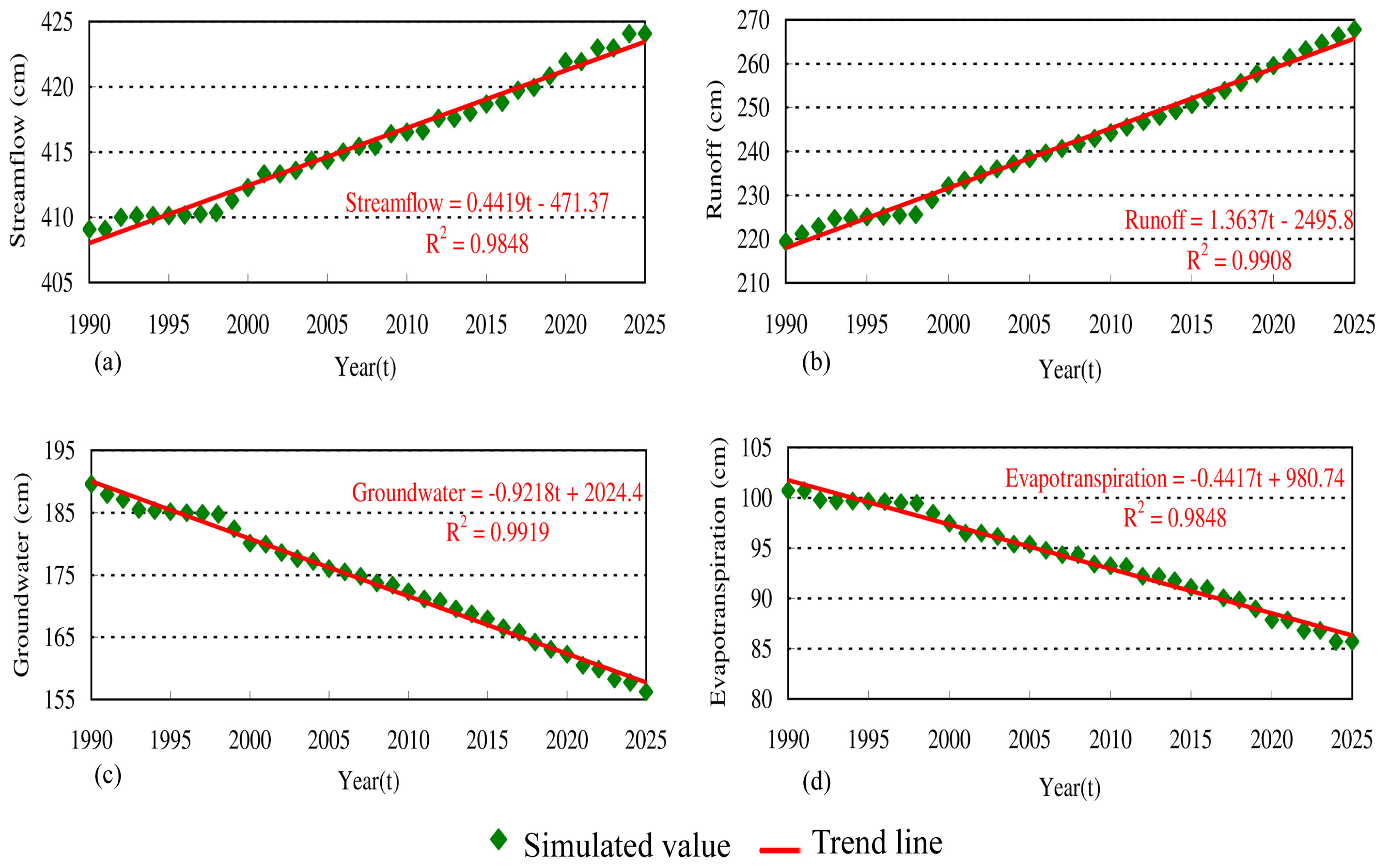
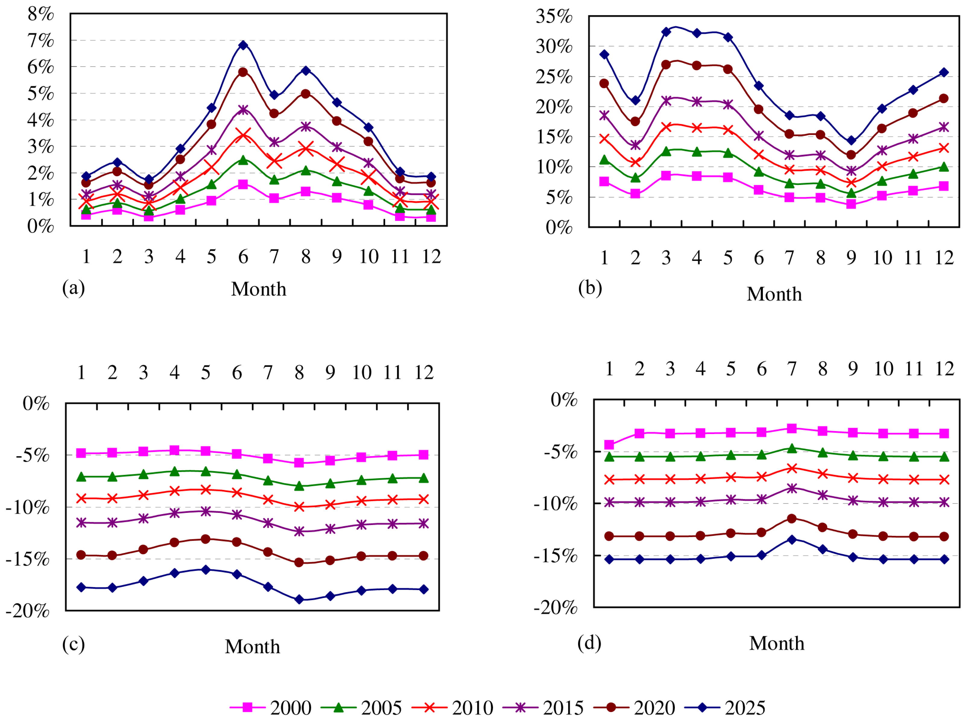
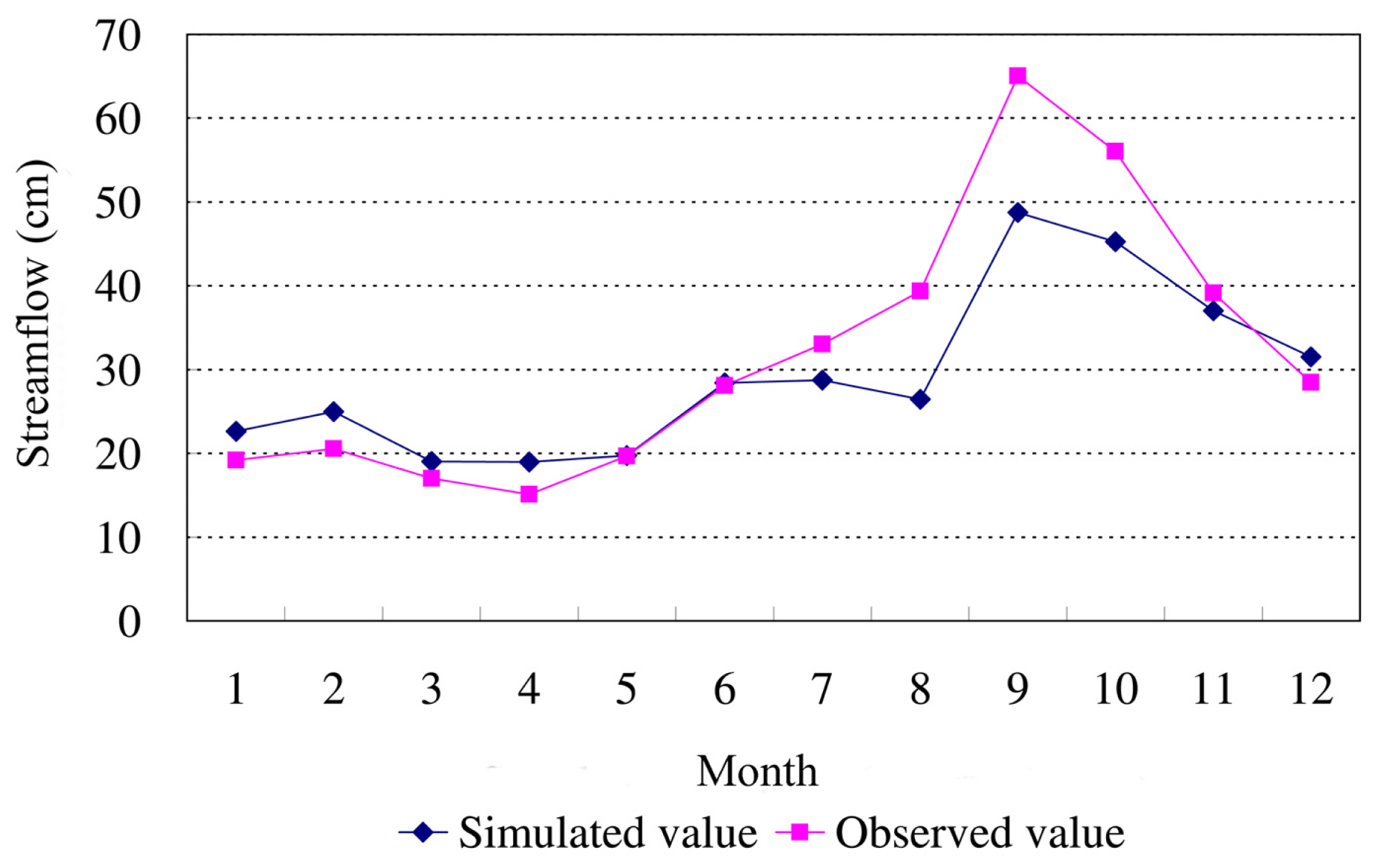
3.3. Historical and predicted hydrology change induced by land-use changes

Based on historical weather data and historical land uses, streamflows, surface runoff, groundwater discharge and evapotranspiration were simulated using the GWLF model and SLEUTH-predicted land-use demands for 1990–2025 for the entire watershed. To compare annual variations in hydrological components, differences in annual streamflow, surface runoff and groundwater discharge based land uses in 1990 (baseline) and hydrological components (based on predicted land uses for 2001–2025) in the entire watershed during the simulation period, annual streamflows, runoff, groundwater discharge and evapotranspiration were calculated based on simulated monthly streamflows, runoff, groundwater discharge and evapotranspiration (Figure 8). Differences in annual streamflow, annual surface runoff, groundwater discharge and evapotranspiration due to land-use change gradually increased to 4.0% and 22.0%, and decreased 18.0% and 15.0%, respectively, during the simulation period (Figure 8).

Figure 9 presents the differences in monthly streamflow, surface runoff, groundwater discharge and evapotranspiration between 1990 and land-use changes in 2005, 2010, 2015, 2020 and 2025. The highest changes in monthly streamflows occurred during May–August 2012, 2016, 2020, and particularly in 2025 when monthly streamflow increased by 7.0% (Figure 9(a)). The peak differences in monthly streamflow between land-use change and no change occurred in June and August of all study years. Peak differences in surface runoff between land use change and no change occurred in March, April and May of each year; in 2025 peak differences were highest (32.0%) (Figure 9(b)). Figure 9(c) shows the differences in monthly groundwater discharge between land-use changes and no change (1990). The greatest decrease (−18.0%) in groundwater discharge occurred in August 2025 (Figure 9(c)). The decrease (−15.0%) in evapotranspiration occurred in all months during 2025, except for June (Figure 9(d)).

4. Discussions

4.1. Land-use change drivers and modeling

Urban dynamic modeling is designed to reproduce observed patterns with high accuracy through capturing the major driving factors that influence urban spatial variations [1]. In CLUE-s modeling, logistic model results for all land uses indicate that the locations of agricultural land are determined by biophysical parameters (altitude, slope and soil erosion coefficients) and socio-economic characteristics, such as distance to major roads, distance to built-up areas, distance to urban planning areas and population density. Moreover, the coefficients of slope and soil erosion (2.1461 and −0.061) in the logistic model for agricultural land were greater than those of other driving factors in the model. This analytical result suggests that agricultural activity is complex and affected by physical and socio-economic characteristics in this watershed, especially slope and soil conditions. The location and distribution of forests are markedly affected by biophysical factors (slope, soil drainage and soil erosion). Coefficients of slope, soil drainage and soil erosion in the logistic model for forest were greater than those of other driving factors in the model. However, regression results confirm that each location has specific soil characteristics influencing the potential for natural and agricultural vegetation [13]. The locations for built-up areas are limited by slope, original built-up areas and population density. Slope of and distance to built-up areas have negative coefficients (−0.020 and −0.0283), suggesting that population pressure caused built-up areas to expand into non-urban areas with low elevations. The locations of grasslands are impacted by all factors except elevation, population density, soil drainage and the soil erosion coefficient. This regression result indicates that grassland distributions, including natural succession and human-made development (e.g., parks and open spaces) are controlled by nature (soil drainage and slope) and human activity. However, most land-use types are impacted by socio-economic factors, suggesting that urbanization impacts the land use in the study watershed. Logistic regression results also confirm that biophysical characteristics have been incorporated as potential benefits achieved via particular land uses at certain locations [13]. Moreover, the soil erosion coefficient was included in all logistic regression models for all land uses, with the exception of the built-up land model. These regression results indicate that soil erosion can drive agricultural land and other land-use changes in the Paochiao watershed.

In the CLUE-s model, slope was included in all logistic regression models, while minimum distance to major roads was included in all logistic regression models except the built-up land model. These regression results indicate that slope and transportation routes can increase urbanization and generate land-use changes in the Paochiao watershed. The SLEUTH model is a simplified model that mainly considers slope and transportation influences on urbanization. The slope factor in the SLEUTH model controls spontaneous urban growth, suggesting that for areas with gentle slopes have an increased probability of spontaneous urbanization. The factor simulates the initial and follow-up urbanization in the vicinity of roads. The relationship between land-use patterns and processes generate land-use changes over time and space [34]. Using a simplified process can fail to delineate complex changes in land-use patterns. As indicated, the SLEUTH model exhibited problems when attempting to capture the allocation of new individual urban patches as part of urban expansion [3].

4.2. land-use patterns of historical and predicted land-uses

The relationship between land-use patterns and processes that form them changes over time and space [16, 35]. Using spatial metrics is beneficial for analyzing urban growth as they provide a comprehensive method for describing a process, comparisons between cities, and comparisons with theory [3]. Therefore, the integrated application of remote sensing, spatial metrics, and urban growth models is an innovative approach for studying spatiotemporal urban growth patterns [3]. In this study, land-use pattern analysis shows that landscape metrics successfully present historical and predicted land-use patterns. Increasing NP, TE and the IJI associated with decreasing MPS, MSI and MNN show that land-use patterns in the watershed tended to fragment, had regular shapes and interspersion patterns, but were relatively less isolated in 1990–2000. Similar to historical land-use patterns, CLUEs-predicted land-use patterns tended to fragment, had regular shapes and interspersion patterns, but were relatively less isolated in 2001–2025 and less interspersed from 2005–2025 compared with land-use pattern in 1990. Conversely, the decrease to NP, TE and MSI associated with increases to MPS and MNN reveal that SLEUTH-predicted land-use patterns in the watershed typically clustered, had regular shapes and isolated patterns in 2001–2025.

Regression equations for landscape metrics with time of CLUE-s- and SLEUTH-predicted land uses were fitted (Figure 7). The values of TE and MPFD exhibited a linear relationship to time in the watershed (Figures 7(e) and 7(f)). The values of NP, MPS, MSI, AWMSI, MNN and the IJI exhibited second-order polynomial relationships with time (Figure 7). These analytical results imply that the land-use model used to predict land-use change processes was dominated by biophysical and human drivers—which operate on distinct spatial and temporal scales—that can generate land-use patterns related to time functions. The regression of landscape matrices during 2001–2025 were used to back forecasts and fit trends in landscape matrices with historical land-use patterns. The mean square errors between the back forecasted and historical landscape matrices during 1990–2000 indicate that the CLUE-s model replicated historical landscape matrices of NP, MPS, TE, and MNN more precisely than did the SLEUTH model (

Table 3. Mean square errors in extrapolated and historical landscape matrices during 1990-2000.

Landscape matrices	SLEUTH model	CLEU-s model
NP	72273.8	14953.1
MPS	2.2	0.2
MSI	0.000	0.001
AWMSI	1.1	1.0
TE	11996.6	1193.7
MPFD	0.00003	0.00003
MNN	171.1	21.9
IJI	0.6	1.4

). Regression results indicate that the CLUE-s model successfully simulated land-use patterns and captured historical land-use patterns in the study watershed during a specific period (Figure 7). Test (t-test) results indicate that landscape matrices, except for MSI, MPFD and the IJI, of landscape patterns determined by two land-use change models were significantly different (

Table 4. t-test of the landscape matrices during 2001-2025.

	CLUE-S model (n=25)	SLEUTH model (n=25)	t-test
NP	1540.28	1219.56	11.125***
MPS	6.4296	8.1432	-10.473***
TE	784777.60	696614.40	8.308***
MSI	1.282	1.2848	-1.247
AWMSI	13.3212	12.4448	4.953***
MPFD	1.04	1.04	N/A
MNN	96.08	114.728	-9.948***
IJI	53.3824	52.8952	0.84

N/A represents not significant;

^‘*’represents p < 0.05 ;

^‘**’represents p < 0.01;

^‘***’represents p < 0.001

). The regression of landscape metrics results indicate that the CLUE-s model effectively predicted land-use patterns and allocated land uses based on suitability of historical land uses in the study watershed. The metrics of SLEUTH-predicted land uses confirm that SLEUTH experiences problems when capturing the allocation of new individual urban patches as part of urban expansion [3]. This analytical finding indicates that SLEUTH did not always predict new urban pixels accurately, nor did it predict the locations of pixels with a high degree of accuracy [3]. These problems are again partly associated with the threshold used in allocating new growth in SLEUTH modeling. The SLEUTH model uses just a few simple metrics (total area growth, number of individual urban patches and edge length) as calibration metrics [3]. However, this study's results support the recommendations by Herold et al. (2003) [3] for further exploration and integration of different spatial metrics specifically useful in representing characteristics of spatial urban growth.

4.3. Impact of land-use changed on hydrology

Understanding the impacts of land-use/land-cover change on hydrologic cycles is required for managing natural resources [36]. A meaningful aggregation of data should first preserve the area percentages of different land-use classes because land-use is the most important data required by a water flux model [37]. In this study, the GWLF model effectively simulated monthly streamflow, surface runoff, groundwater discharge and evapotranspiration under no land-use change and accurately predicted land-use change conditions. The predicted hydrological components (streamflow, surface runoff, groundwater discharge and evapotranspiration) were impacted by predicted land-use changes under land-use change pressure (urban sprawl). Runoff from built-up areas increased and groundwater discharge decreased as replacement of vegetation with development reduced infiltration. Land-use change increased peak differences in streamflow, surface runoff, groundwater discharge, and streamflow variability. Peak differences in surface runoff between 1990 land use and land use in each simulated year occurred in April and July, as these months typically have minimal precipitation. Peak differences in streamflow between 1990 land use and land use in each simulated year occurred on during periods of low precipitation (May–August), primarily because of land-use change, especially in 2025. During the simulation periods, yearly cumulative changes of surface runoff, groundwater discharge, evapotranspiration and streamflow in the study watershed were 22.0%, 17.6%, 15.0% and 4.0 %, respectively. Moreover, monthly streamflows were dominated by groundwater discharge in March and April in 1999; however, land-use changes in monthly streamflows are equally dominated by groundwater discharge and surface runoff in March and April 2025. The highest difference between 1990 and 2025 (impacts) of urbanization for monthly streamflow, monthly surface runoff, monthly groundwater discharge and monthly evapotranspiration were 6.0%, 32.0%, 18.0% and 15.0%, respectively. The impacts of land-uses changes (urbanization) on hydrology were proportional to the degree of urbanization. Hydrological modeling results suggest that hydrology and interactions of hydrological components are significantly impacted by land-use changes. The degrees of impacts due to urbanization on monthly hydrological components respectively are surface runoff, groundwater discharge, evapotranspiration and streamflow.

4. Conclusions

The impacts of changes in land-use patterns on hydrology caused by urbanization of watersheds are crucial issues in watershed land-use planning and water resource management. Integrating effective models and useful historical data to accurately capture historical land-use and predict land-use changes and hydrology caused by urbanization is effective in watershed land-use planning and water resource management. This study integrated remote-sensing data, an urban sprawl model, a land-use change model, landscape metrics, and a hydrological model to predict and assess future land-use patterns and hydrological processes under urbanization pressure in the Paochiao watershed, Taiwan. The remote-sensing data provided sufficient information for analyzing and predicting urbanization in the watershed. The bottom-up urban growth model, SLEUTH, and the top-down land-use change model, CLUE-s, predicted land-use changes and captured historical land-use patterns caused by urbanization in the watershed during 1999–2025; the CLUE-s model precisely captured historical land-use patterns of urbanization in the study watershed. The landscape metrics accurately represent land-use patterns and are useful tools for assessing the capabilities of land-use models for historical and predicted land-use patterns that tended to fragment, had regular shapes and relative less isolated patterns in the Paochiao watershed. These metrics can be integrated into the urban growth model calibration process and land-use change allocation processes to limit predicted land-use patterns based on historical land-use patterns. The GWLF hydrological model provided useful information for predicting the impacts of urbanization for the study watershed. The impacts of urbanization on hydrology and interactions of hydrological components are proportional to the levels of urbanization in the study watershed. The degrees of impacts of urbanization on monthly and yearly hydrological components respectively are surface runoff, groundwater discharge, evapotranspiration and streamflow.

References

1. Xian, G.; Crane, M.; Steinwand, D. Dynamic modeling of Tampa Bay urban development using parallel computing. Computers and Geosciences 2005, 31(7), 920–928. [Google Scholar]
2. Fang, S.; Gertner, G.Z.; Sun, Z.; Anderson, A.A. The impact of interactions in spatial simulation of the dynamics of urban sprawl. Landscape and Urban Planning 2005, 73(4), 294–306. [Google Scholar]
3. Herold, M.; Goldstein, N.C.; Clarke, K.C. The spatiotemporal form of urban growth: measurement, analysis and modeling. Remote Sensing of Environment 2003, 86(3), 286–302. [Google Scholar]
4. Batty, M.; Howes, D. Remote sensing and urban analysis. In Predicting temporal patterns in urban development from remote imagery; Donnay, J.P., Barnsley, M.J., Longley, P.A., Eds.; Taylor and Francis: London and New York, 2001; pp. 185–204. [Google Scholar]
5. Jensen, J.R.; Cowen, D.C. Remote sensing of urban/suburban infrastructure and socio-economic attributes. Photogrammetric Engineering and Remote Sensing 1999, 65(5), 611–622. [Google Scholar]
6. Herold, M.; Menz, G.; Clarke, K.C. Remote Sensing and Urban Growth Models – Demands and Perspectives. In Regensburger Geographische Schriften, Symposium on remote sensing of urban areas, Regensburg, Germany, June 2001; 2001; 35. [Google Scholar]
7. Hietel, E.; Waldhardt, R.; Otte, A. Analysing land-cover changes in relation to environmental variables in Hesse, Germany. Landscape Ecology 2004, 19(5), 473–489. [Google Scholar]
8. Lin, Y.P.; Hong, N.M.; Wu, P.J.; Lin, C.J. Modeling and assessing land-use and hydrological processes to future land-use and climate change scenarios in watershed land-use planning. Environmental Geology 2007, 53(3), 623–634. [Google Scholar]
9. Agarwal, C.; Green, G.M.; Grove, J.M.; Evans, T.P.; Schweik, C.M. A Review and Assessment of Land-use Change Models: Dynamics of Space, Time, and Human Choice; US Dept. of Agriculture, Forest Service, Northeastern Research Station, 2002; pp. 12–27. [Google Scholar]
10. Dietzel, C.; Clarke, K.C. Toward Optimal Calibration of the SLEUTH Land Use Change Model. Transactions in GIS 2007, 11(1), 29–45. [Google Scholar]
11. Verburg, P.H.; Veldkamp, A. Projecting land use transitions at forest fringes in the Philippines at two spatial scales. Landscape Ecology 2004, 19(1), 77–98. [Google Scholar]
12. Verburg, P.H.; De Nijs, T.C.M.; Ritsema Van Eck, J.; Visser, H.; De Jong, K. A method to analyse neighbourhood characteristics of land use patterns. Computers, Environment and Urban Systems 2004, 28(6), 667–690. [Google Scholar]
13. Verburg, P.H.; Ritsema Van Eck, J.R.; De Nijs, T.; Dijst, M.J.; Schot, P. Determinants of land use change patterns in the Netherlands. Environment and Planning B 2004, 31(1), 125–150. [Google Scholar]
14. Overmars, K.P.; de Koning, G.H.J.; Veldkamp, A. Spatial Autocorrelation in Multi-scale Land Use Models. Ecological Modelling 2003, 164, 257–270. [Google Scholar]
15. Dietzel, C.; Clarke, K.C. Spatial Differences in Multi-Resolution Urban Automata Modeling. Transactions in GIS 2004, 8(4), 479–492. [Google Scholar]
16. Jantz, C.A.; Goetz, S.J. Analysis of scale dependencies in an urban land-use-change model. International Journal of Geographical Information Science 2005, 19(2), 217–241. [Google Scholar]
17. Syphard, A.D.; Clarke, K.C.; Franklin, J. Using a cellular automaton model to forecast the effects of urban growth on habitat pattern in southern California. Ecological Complexity 2005, 2(2), 185–203. [Google Scholar]
18. Verburg, P.H.; Schulp, C.J.E.; Witte, N.; Veldkamp, A. Downscaling of land use change scenarios to assess the dynamics of European landscapes. Agriculture, Ecosystems and Environment 2006, 114(1), 39–56. [Google Scholar]
19. Castella, J.C.; Pheng Kam, S.; Dinh Quang, D.; Verburg, P.H.; Thai Hoanh, C. Combining top-down and bottom-up modelling approaches of land use/cover change to support public policies: Application to sustainable management of natural resources in northern Vietnam. Land Use Policy 2007, 24(3), 531–545. [Google Scholar]
20. Dietzel, C.; Clarke, K.C. The effect of disaggregating land use categories in cellular automata during model calibration and forecasting. Computers, Environment and Urban Systems 2006, 30(1), 78–101. [Google Scholar]
21. Lin, Y.P.; Hong, N.M.; Wu, P.J.; Wu, C.F.; Verburg, P.H. Impacts of land use change scenarios on hydrology and land use patterns in the Wu-Tu watershed in Northern Taiwan. Landscape and Urban Planning 2007, 80(1-2), 111–126. [Google Scholar]
22. Turner, M.G.; Gardner, R.H.; O'Neill, R.V. Landscape Ecology in Theory and Practice: Pattern and Process; Springer: New York, 2001; pp. 108–109. [Google Scholar]
23. Botequilha Leitao, A.; Ahern, J. Applying landscape ecological concepts and metrics in sustainable landscape planning. Landscape and Urban Planning 2002, 59(2), 65–93. [Google Scholar]
24. Corry, R.C.; Nassauer, J.I. Limitations of using landscape pattern indices to evaluate the ecological consequences of alternative plans and designs. Landscape and Urban Planning 2005, 72(4), 265–280. [Google Scholar]
25. Legesse, D.; Vallet-Coulomb, C.; Gasse, F. Hydrological response of a catchment to climate and land use changes in Tropical Africa: case study South Central Ethiopia. Journal of Hydrology 2003, 275(1-2), 67–85. [Google Scholar]
26. Haverkamp, S.; Fohrer, N.; Frede, H.G. Assessment of the effect of land use patterns on hydrologic landscape functions: a comprehensive GIS-based tool to minimize model uncertainty resulting from spatial aggregation. Hydrological Processes 2005, 19(3), 715–727. [Google Scholar]
27. Fohrer, N.; Haverkamp, S.; Frede, H.G. Assessment of the effects of land use patterns on hydrologic landscape functions: development of sustainable land use concepts for low mountain range areas. Hydrological Processes 2005, 19(3), 659–672. [Google Scholar]
28. Haith, D.A.; Shoemaker, L.L. Generalized watershed loading functions for stream flow nutrients. Water Resources Bulletin 1987, 23(3), 471–478. [Google Scholar]
29. Clarke, K.C. Land Transition Modeling With Deltatrons. Proc. The Land Use Modeling Conference, Sioux Falls, SD, June 1997.
30. Claggett, P.R.; Jantz, C.A.; Goetz, S.J.; Bisland, C. Assessing Development Pressure in the Chesapeake Bay Watershed: An Evaluation of Two Land-Use Change Models. Environmental Monitoring and Assessment 2004, 94(1), 129–146. [Google Scholar]
31. Verburg, P.H.; Soepboer, W.; Veldkamp, A.; Limpiada, R.; Espaldon, V.; Mastura, S.S.A. Modeling the Spatial Dynamics of Regional Land Use: The CLUE-S Model. Environmental Management 2002, 30(3), 391–405. [Google Scholar]
32. Elkie, P.C.; Rempel, R.S.; Carr, A.P. Patch analyst user's manual. A tool for quantifying landscape structure. Ont. Min. Natur. Resour. Northwest Sci. and Technol. Thunder Bay, Ont. Technical Manual TM-002 1999, 4–12. [Google Scholar]
33. Mcgarigal, K.; Marks, B.J. FRAGSTATS: Spatial Pattern Analysis Program for Quantifying Landscape Structure; Portland, Or.; US Dept. of Agriculture, Forest Service, Pacific Northwest Research Station, 1995; pp. 38–53. [Google Scholar]
34. Carlile, D.W.; Skalski, J.R.; Batker, J.E.; Thomas, J.M.; Cullinan, V.I. Determination of ecological scale. Landscape Ecology 1989, 2(4), 203–213. [Google Scholar]
35. Gibson, C.C.; Ostrom, E.; Ahn, T.K. The concept of scale and the human dimensions of global change: a survey. Ecological Economics 2000, 32(2), 217–239. [Google Scholar]
36. Scanlon, B.R.; Reedy, R.C.; Stonestrom, D.A.; Prudic, D.E.; Dennehy, K.F. Impact of land use and land cover change on groundwater recharge and quality in the southwestern US. Global Change Biology 2005, 11(10), 1577–1593. [Google Scholar]
37. Bormann, H. Impact of spatial data resolution on simulated catchment water balances and model performance of the multi-scale TOPLATS model. Hydrology and Earth System Sciences 2006, 10(2), 165–179. [Google Scholar]
Figure 1. Land use patterns in 2000 and the location of the Paochiao watershed.
Sensors 08 00658f1
Figure 2. Land-uses of the Paochiao watershed in (a) 1990; (b) 1993; (c) 1998; (d) 2000.
Sensors 08 00658f2
Figure 3. Mean monthly stream flow.
Sensors 08 00658f3
Figure 4. SLEUTH simulated land use spatial distribution in Paochiao watershed (a)2005 (b)2010 (c)2015 (d)2020 and (e)2025 year.
Sensors 08 00658f4
Figure 5. Predicted Land uses of the SLEUTH model.
Sensors 08 00658f5
Figure 6. The CLUE-s simulated land-use distribution in Paochiao watershed in (a) 2005, (b) 2010, (c) 2015, (d) 2020, and (f) 2025.
Sensors 08 00658f6
Figure 7. The fitting results of the predicted landscape matrices of (a)NP, (b)MPS, (c)MSI, (d)AWMSI, (e)TE, (f)MPFD, (g)MNN, and (h)IJI using the CLUE-s and the SLEUTH models, and the comparison between the extrapolating results and the historical landscape matrices.
Sensors 08 00658f7
Figure 8. The annual changes in (a) stream flow, (b) surface runoff (c) groundwater discharge, and (d) evapotranspiration due to land-use changes in the watershed.
Sensors 08 00658f8
Figure 9. The monthly changes in (a) streamflows, (b) surface runoffs, (c) groundwater discharges, and (d) evapotranspiration due to land-use changes in the watershed 3.4. Discussions.
Sensors 08 00658f9