An Automatic Instrument to Study the Spatial Scaling Behavior of Emissivity

Abstract

In this paper, the design of an automatic instrument for measuring the spatial distribution of land surface emissivity is presented, which makes the direct in situ measurement of the spatial distribution of emissivity possible. The significance of this new instrument lies in two aspects. One is that it helps to investigate the spatial scaling behavior of emissivity and temperature; the other is that, the design of the instrument provides theoretical and practical foundations for the implement of measuring distribution of surface emissivity on airborne or spaceborne. To improve the accuracy of the measurements, the emissivity measurement and its uncertainty are examined in a series of carefully designed experiments. The impact of the variation of target temperature and the environmental irradiance on the measurement of emissivity is analyzed as well. In addition, the ideal temperature difference between hot environment and cool environment is obtained based on numerical simulations. Finally, the scaling behavior of surface emissivity caused by the heterogeneity of target is discussed.

1. Introduction

Land surface temperature (LST) is an important parameter governing energy balance over land and an essential determinant driving dynamic change of earth resources and environment and the satellite based LST data is used widely in water cycling studies (Su, et al, 2000a; 2005 and 2007). Emissivity of natural surfaces is an important parameter which relates closely to the determination of LST in the thermal infrared (TIR) remote sensing (Becker, 1987; Rubio et al, 1997). The biggest challenge in the TIR remote sensing is how to separate the surface emissivity and the surface temperature. At present, split window method is used often to solve this problem. Split window algorithm was originally developed for sea surface temperature mapping from NOAA-AVHRR data in 1970s. Spatial distribution of the thermal emissivity of sea surface is much more identical than that of land surface where heterogeneity is a common feature, which makes the solution of LST from thermal radiance transfer equation much more complicated for terrestrial areas. In addition, two essential parameters (atmospheric transmittance and ground emissivity) are required to be known as the premier of LST estimation using split window algorithms (Coll et al., 1994; Qin el al., 2001). Usually estimation of the two parameters is with some errors due to many uncertainty factors such as atmospheric profile data. Even if the properties of the atmosphere profile are known, for a radiometer with N channels, there will be N+1 unknowns (N emissivities plus one surface temperature) in N thermal radiation balance equations based on N radiance measurements. Therefore this system has no unique solution, unless additional independent information is provided (Li, et al, 1999). Different assumptions have to be made to reduce the number of unknowns, for example, the temperature-emissivity separation method (Gillespie, et al,. 1998), the grey body emissivity method (Barducci and Pippi, 1996), and the day/night method (Becker and Li, 1990; Watson, 1992a; Wan and Li, 1997). However, to validate the above assumptions and the emissivity retrievals, direct emissivity measurements or estimations are highly necessary. Furthermore, it was reported that emissivity retrievals are dependent on the spatial resolution and there exists scaling problem due to surface heterogeneity (Moran, et al. 1997; Liu, et al. 2006; Wan, et al. 2002). Therefore, spatial distribution of surface emissivities is very important. Direct operational measurement of emissivity from space has not been demonstrated, although the conceptual design of emissivity measurement using carbon dioxide laser at 10.6 μm on aero-board to measure distribution of surface emissivities was presented (Zhang, 1989) nearly two decades ago. Ground measurements of emissivity including both field and laboratory experiments, provide very useful priori knowledge which can benefit the thermal infrared remote sensing from space (Nerry et al, 1988). Up to now, many approaches of ground measurements have been presented to measure the emissivity, which include box method (Buettner and Kern, 1965; Sobrino and Caselles, 1993), fourier transform infrared spectrometer (FTIR) method (Nerry et al, 1988, 1990; Rivard et al, 1995), CO₂ laser method (Nerry,et al, 1991). In these in situ measurements, particular attention was often given to instrument calibration and the correction of the environmental radiation because of their importance in the determination of emissivity. However, the spatial distribution of surface emissivities was not studied sufficiently in the previous studies. To meet this requirement, an automatic instrumentation was specially designed to measure the spatial distribution of emissivity and to study scaling problem of emissivity and temperature. The details of the instrument will be described in this paper. It has to be pointed that the same instrument was previous used in the experiments (Zhang, et al., 2004) by our group to do the spatial scaling behavior study of surface temperature based on a different experiment strategy. The improvements include: a) A reference box to determine the hot and cool environment irradiance; b) The emissivity of the reference box is known; c) The surface temperature of the box is not adjusted; d) new materials are used as samples in the measurement.

In the paper, the methodology of the emissivity measurements and the design of the instrument are presented in Section 2, followed by the description of the measuring procedures in Section 3. Then, the sensitivity of the measured emissivity induced by the four critical factors is analyzed based on a series of carefully designed experiments: a) quantifying the uncertainty of retrieving ambient radiance; b) evaluating the influence of the ambient radiance, the variation of the sample's temperature and the emissivity of reference box on the measurements; c) determining the ideal temperature difference between hot environment and cool environment, and the best conditions for determining sample emissivity with the instrument. Finally, the potential of using this instrument to study the scaling behaviors of surface emissivity and surface temperature caused by the heterogeneity of target was discussed.

2. Methodology

According to the thermal radiation balance equation, the measured radiance includes a reflection term from the environment (see equation 1). The environment irradiance must be measured before the true surface temperature and the precise measurements of TIR emissivities in the laboratory or in the field can be achieved (Rivard et al, 1995).

$$M(T_{\mathit{\text{rad}}},\lambda )={\mathit{\varepsilon }}_{\lambda }B(T_s,\lambda )+(1-{\mathit{\varepsilon }}_{\lambda })B(T_{\mathit{\text{envi}}},\lambda )$$

(1)

where, M(T_rad,λ) is the radiance from the objects at wavelength λ and T_rad is the radiative temperature. ε_λ is the emissivity of the sample, B(T_s,λ) is Planck's radiation function at the sample temperature, T_s for wavelength λ and B(T_envi,λ) is the irradiance coming from the environment and T_envi is the effective environmental temperature. Please be noted that T_envi is an equivalent temperature, which is introduced to simply equation. In the above equation, it is assumed that the reflection is Lambertian and the consideration of multi-scattering is omitted.

Even the ambient radiance B(T_envi,λ) is known, the ε_λ and T_s can not be solved from only one equation. One feasible solution is to change the ambient radiance and then an additional equation can be obtained, for example, one measurement is performed under the clear sky, the other is inside cloth chamber (Zhang, et al. 2004); or one is acquired with the illumination of CO₂ laser beam and the other is under clear sky (Zhang, et al. 1989; Nerry, et al. 1991). The first method was adopted in our work.

When using a broadband (8–14 μm) thermal camera in this work, sample emissivity can be obtained through four sequences of measurements of radiance:

$$M_{r,8-14\mu m}(T_1)={\mathit{\varepsilon }}_{r,8-14\mu m}{B}_{8-14\mu m}(T_r)+(1-{\mathit{\varepsilon }}_{r,8-14\mu m})B_{8-14\mu m}(T_h)$$

(2)

$$M_{s,8-14\mu m}(T_2)={\mathit{\varepsilon }}_{s,8-14\mu m}{B}_{8-14\mu m}(T_{s2})+(1-{\mathit{\varepsilon }}_{s,8-14\mu m})B_{8-14\mu m}(T_h)$$

(3)

$$M_{r,8-14\mu m}(T_3)={\mathit{\varepsilon }}_{s,8-14\mu m}{B}_{8-14\mu m}(T_{s3})+(1-{\mathit{\varepsilon }}_{s,8-14\mu m})B_{8-14\mu m}(T_c)$$

(4)

$$M_{r,8-14\mu m}(T_4)={\mathit{\varepsilon }}_{r,8-14\mu m}{B}_{8-14\mu m}(T_r)+(1-{\mathit{\varepsilon }}_{r,8-14\mu m})B_{8-14\mu m}B(T_c)$$

(5)

where M_r, _{8–14 μm} (T₁) and M_r, _{8–14 μm} (T₄) are the radiances from reference box in ‘hot’ environment and in ‘cool’ environment measured respectively by the thermal camera. M_s, _{8–14 μm} (T₂) and M_r, _{8–14 μm} (T₃) are the radiances from the sample in ‘hot’ environment and in ‘cool’ environment integrated in the bandwidth of 8–14 μm respectively. T is the temperature, subscript h and c represent ‘hot’ environment and ‘cool’ environment equivalent temperature, subscript s and r represent target object and reference box, respectively. B_{8–14 μm} (T) is Planck's radiation function at the sample temperature T integrated over the bandwidth of 8–14 μm. Because the change of hot and cool environments is done within several seconds, the temperature variation of the object can be neglect. Assuming T_s2= T_s3 and eliminating the radiance emitted by the target itself from Eq.(3) and Eq.(4), the emissivity of the sample in the bandwidth of 8 – 14 μm can be obtained by Eq.(6), which is an effective emissivity for a broad bandwidth (Su, et al., 2000b). It has to be noted that time interval between the second measurement M_s, _{8–14 μm} (T₂) and the third measurement M_s, _{8–14 μm} (T₃) must be controlled as short as possible to ensure T_s2= T_s3. Using the instrument in our work, time interval is no longer than about 5s, which can justify the assumption of the constant temperature of the object, especially for the sample with large thermal inertia.

$${\mathit{\varepsilon }}_{s,8-14\mu m}=1-\frac{M_{s,8-14\mu m}(T_2)-M_{s,8-14\mu m}(T_3)}{B_{8-14\mu m}(T_h)-B_{8-14\mu m}(T_c)}$$

(6)

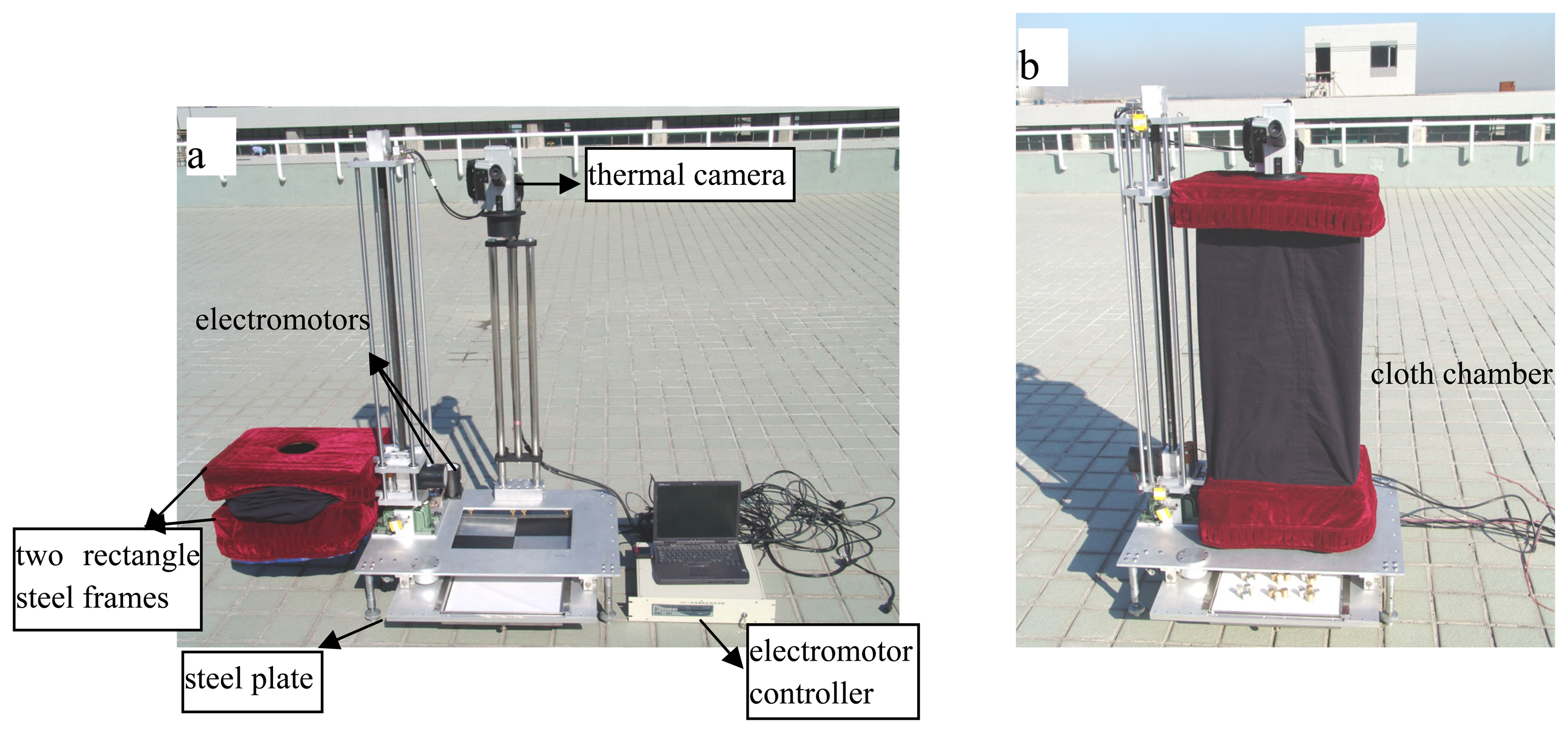
The instrument was designed to implement the above algorithm showed in Figure. 1. It is composed of four parts: a) horizontal moving equipments, mainly including a steel plate on which hollow reference box and the samples can be put on it in the experiment. This part is designed to control the horizontal moving of the steel plate and is used to put the sample and the reference box under the view field of the thermal camera alternatively; b) horizontal rotating equipments, mainly including two rectangle steel frames on which the cloth chamber is fixed. The upper one can move in vertical direction and the lower one is fixed at a constant height. There is a central hole on the top of the cloth chamber through which radiometric measurements can be taken. This part is used to make the cloth chamber rotate in horizontal 180 azimuth angle, which controls the alternation of ‘hot’ environment (inside the cloth chamber) and ‘cool’ environment (outside the cloth chamber, namely sky environment); c) vertical moving equipments, it controls the vertical moving of the upper steel frame and stretching the cloth chamber and making the ‘hot’ environment. The above three components are all made of stainless steel, which makes the instrument durable in the field experiments. All movements of the three parts are driven by electromotor, so there are total three electromotors in the system. d) automatic controlling equipments, including a notebook computer and an electromotor controller. It is mainly used to control the behaviors of the three electromotors and the observation of thermal camera by means of a C++ program.

Using the above four parts, the whole system works in the following way step by step:

1)

putting the sample and the reference box in the steel plate and opening the thermal camera;

2)

under the driving of horizontal rotating equipments, the cloth chamber is situated over the reference box;

3)

under the drive of vertical moving equipments, the cloth chamber is stretched up and the ‘hot’ environment is made, after one second, the first measurement M_r, _{8–14 μm} (T₁) is performed;

4)

switching the measured object from reference box to the sample by horizontal moving equipments, the second measurement M_r, _{8–14 μm} (T₂) is completed;

5)

dropping the cloth chamber and rotating it off the sample by vertical moving equipments and horizontal rotating equipments as fast as possible, after one second, the third measurement M_r, _{8–14 μm} (T₃) is obtained;

6)

switching the measured object from the sample to reference box by horizontal moving equipments, the fourth measurement M_r, _{8–14 μm} (T₄) is acquired.

The whole operation is performed automatically and takes about 15 seconds totally. So the instrument is very convenient to operate. Low irradiance of the sky on a clear day and relatively high irradiance of a cloth chamber above the object are used to supply two different environmental irradiances, which is a prerequisite to directly measure emissivity from emission of surface.

For the measurement of temperature, we used a non-frozen thermal camera, which operates in the 8-14 μm spectral window with a temperature sensitivity of 0.1K. The dimension of every thermal image is 320×240. Its response time ranges between l/50s and l/60s. The pixel size will varies according to the distance between the thermal camera and the target object. The thermal camera was installed on the trestle table at height of 1.3m above the target object, so one image covered 0.4m×0.3m area. In the four measurements, three images per measurement were obtained with 0.23s interval time in case of bad image. For the same sample, we repeated the measurements for three times to ensure the validity of data.

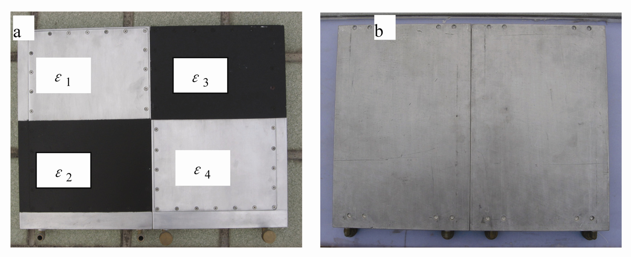
For calculating the ambient radiance, the reference boxes with known emissivities were used, which is shown in Figure.2. It consisted of two hollow boxes made of aluminium. One half upper surface of every box was sprayed with a layer of black lacquer with high emissivity about 0.98. The other half and its undersurface were polished to grey-white body with an average surface roughness of 2-5 urn which can give low emissivity about 0.3 without specular reflection. The first value of emissivity is given by the manufacturer of the black paint; the second one has been determined by means of a portable instrument for measuring emissivity which has been validated in previous applications (Patent no, ZL 02 1 23745.X). There is a hole on the upper surface of every box, through which water with some temperature can be poured into it to make the box an isothermal surface and to control the surface temperature of the box. The size of reference boxes is 0.4m length and 0.3m width, which is determined according to the installation height and view field of the thermal camera.

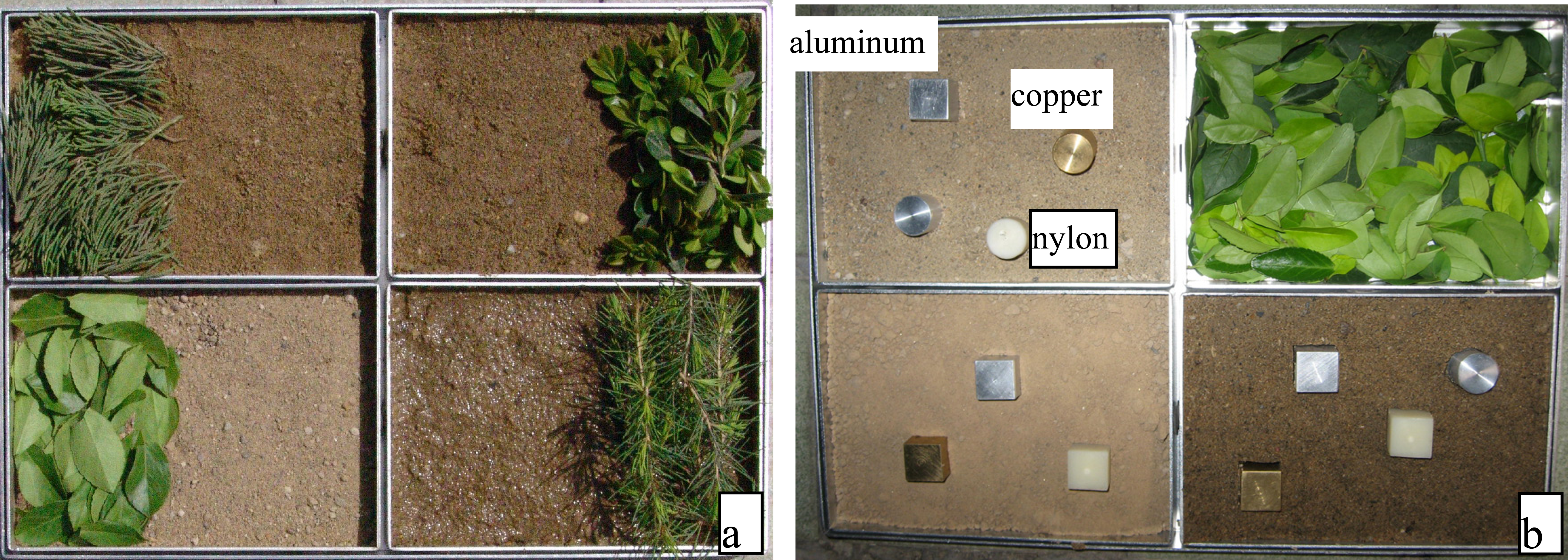
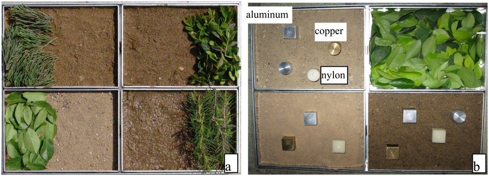
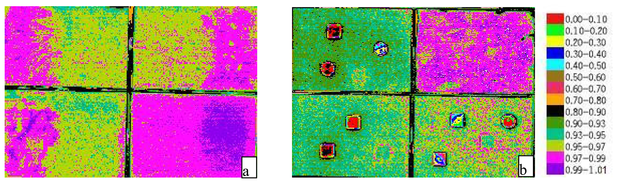
Another important component of the system is the sample plate. It is composed by four rectangle salvers; thereby different samples can be put in different salvers and can be observed at one time. Thus, using the thermal camera, spatial distribution of the thermal radiation of the samples can be obtained, which makes possible the study of the scaling behavior of the emissivity and the true surface temperature. Figure.3 shows two of the samples used in our experiments. In figure.3a, Silver sand with four different water content and some vegetation leaves were put in the salvers, where the lower-right soil is the wettest, the lower-left soil is the driest and upper-right soil is wetter than upper-left soil. In figure.3b, Silver sand, agricultural soil, vegetation leaves and wet sandy soil were put in the upper-left salver, lower-left salver, upper-right salver and lower-right salver, respectively, and some metal blocks made of aluminum, copper and nylon were inserted in the soils. Thus, the configuration of large emissivity difference was built up, which provides great benefit for validating the system and the study of the emissivity scaling.

From Eq.(6) we can see that ambient radiance, B_{8–14 μm} (T_h) and B_{8–14 μm} (T_c), must be calculated firstly. According to Eq.(2) or Eq.(5), there are two methods: (a) if the surface temperature of reference box, T_r, is known by measuring the temperature of the water inside, and in terms of the value of M_r, _{8–14 μm} (T₁) and ε_r, _{8–14 μm}, B_{8–14 μm} (T_h) of every Pixel would be obtained using Eq.(2); (b) if T_r can't be acquired, using the difference between the emissivity of reference box painted in black lacquer and the emissivity of polished aluminium, two equations as Eq.(2) could be established for the same environment, based on which, the emittance from reference box and the average radiance from the environment can be solved. Similarly, B_{8–14 μm} (T_c) can also be solved. Evidently, ambient radiance of every pixel can be obtained using the former method, but only average ambient radiance can be acquired using the latter method. It will produce different emissivity results using the two different ambient radiances due to the heterogeneity of ambient radiance. This problem will be discussed in detail in the following sections.

3. Emissivity Measurements

For avoiding the effects of shadows of the instruments on the measurements and calculations, we did the experiments after sun set on Jul 20 and Aug 11, 2007. Figure.4 is the results of two of the samples showed in Figure.3 according to the above methodology.

From Figure.4a, it can be seen that soil emissivity increases with the increase of soil water content. The average emissivity from driest soil to wettest soil is 0.9514, 0.9589, 0.9639 and 0.9803, respectively. Their standard deviations are 0.0008, 0.0065, 0.0061 and 0.0049. Vegetation emissivity is about 0.9847. For Figure.4b, the emissivities of copper and aluminum are obviously smaller than soil and vegetation, and dry sandy soil has the lowest emissivity value, about 0.9421; vegetation has the highest value, about 0.9827. The results appear to be in a reasonable range.

4. Analysis of Sensitivity in the Method

In terms of the procedures of measuring emissivity, there are four principal factors in the estimation of uncertainty in emissivity. All the discussions below are specifically for the bandwidth of 8–14 μm by default. To simplify the symbols, 8–14 μm in the subscript is omitted.

(1)

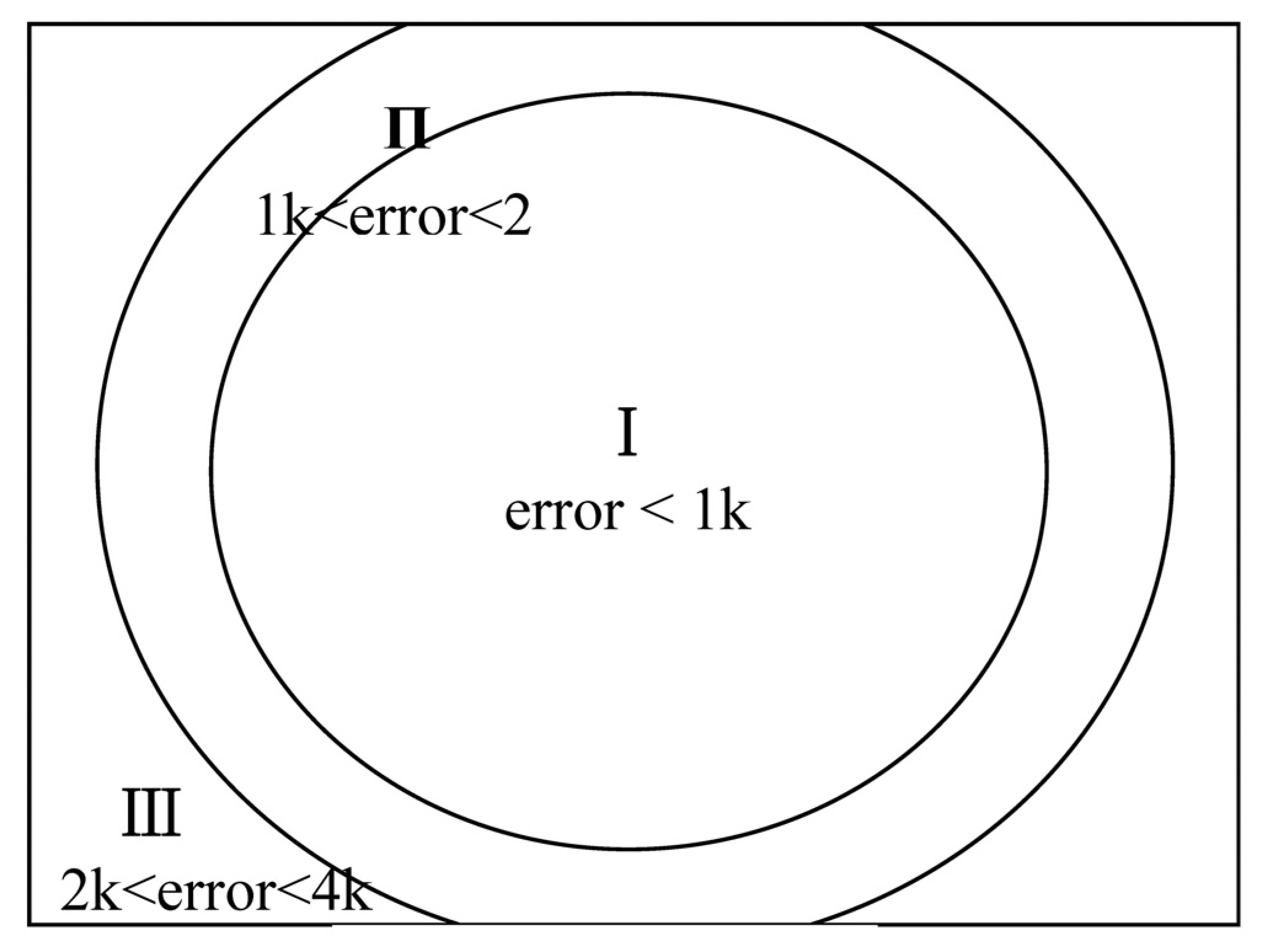
M, the measured apparent radiance. The uncertainty in M is primarily from the thermal camera itself. Using the blackbody as the sample, we analyzed the characteristics of the thermal camera. Note that, in the measurements, although an auto-adjust function for correcting the temperature drift was set, there still was 4k drift errors at most in one regulating period, moreover, we found that there was almost no error for the central part of the thermal image, while with the increase of the distance from the central, the error increased and can reach 4k, that is to say, there are large errors for the pixels around the edge of the thermal image. According to the magnitude of the errors, the thermal image can be grouped into three regions as shown in Figure.5. The percentage (I) of drift error less than Ik was about 50% and the percentage (II and III) of the other two groups was about 25%, respectively. In order to reduce this error, in terms of the view field of the camera, we installed it at height of 1.3m to make the sample locate in the region of I and II. At the same time, we also calibrated the thermal camera using the blackbody in the experiments.

(2)

T_envi, environmental temperature, is calculated from Eq.(2) and Eq.(5). Obviously, T_envi is determined by the emitting radiance of target object B_{8_14 μm} (T_r), the radiance from the surface M_r and the emissivity of reference box ε_r according to Eq.(2) or Eq.(5). In terms of our simulations, it is found that ambient radiance is more sensitive to B_{8_14 μm} (T_r) and M_r for the reference box of high emissivity than that for the reference box of low emissivity.

Table 1. Sensitivies of T_envi to T_rad and T_r for different ε_r

Trad	Tenvi(Tr= 300.71)			Tr	Tenvi(Trad= 301.15)
	εr= 0.98	εr = 0.75	εr = 0.3		εr = 0.98	εr = 0.75	εr = 0.3
301.15	320.8532	302.4712	301.3398	296.5	424.7418	313.9419	303.0786
301.25	324.9119	302.8654	301.4824	297	416.128	312.6673	302.8772
301.35	328.8277	303.2585	301.6249	297.5	406.8952	311.3704	302.6745
301.45	332.6122	303.6504	301.7673	298	396.9354	310.0504	302.4703
301.555	336.2753	304.0412	301.9097	298.5	386.1071	308.7065	302.2646
301.65	339.8259	304.4309	302.052	299	374.2201	307.3379	302.0575
301.75	343.272	304.8195	302.1943	299.5	361.0087	305.9438	301.8489
301.85	346.6206	305.207	302.3365	300	346.0837	304.5232	301.6388

shows the simulated results. The left four columns represent the variation of T_envi with T_rad, for different ε_r and T_r = 300.71. In this case, it can be seen that 0.1k variation in the value of T_rad results in variations of approximately 4k, 0.4k, 0.15k in T_envi for different surface emissivities, respectively, calculated with Eq.(2). That is to say, for high surface emissivity, such as reference box painted black lacquer, only a little variation of T_rad would induce large variation of T_envi. The right four columns represent the variation of T_envi with T_r, we can see that for high surface emissivity, a 0.5k increase in the value of T_r produced about 9k decrease of T_envi, but for low surface emissivity (0.3), only a 0.2 decrease of T_envi was generated. Above all, it can be concluded that T_envi is more sensitive to T_rad and T_r for high surface emissivity than that for low surface emissivity. For this reason, in the experiment, low surface emissivity should be adopted to calculate the ambient radiance. Because the half upper surface emissivity of our reference box is painted by black lacquer with high emissivity about 0.98, we used its undersurface to retrieve the ambient radiance, with an emissivity value of ε_r≈ 0.3, seen from Figure. 3.

In addition, as the above section said, the radiance from the environment exhibits great heterogeneous, so only using the average ambient radiance to retrieve emissivity must produce some errors. For quantitatively evaluating and clarifying this effect on the calculation of emissivity, we specially did the following analysis based on our experimental data.

Table 2. Average T_envi and the standard deviation of it in ‘hot’ environment and in ‘cool’ environment.

Measuring Date	Data group	average_Th	std_Th	average_Tc	std_Tc
11/8/2007	Group1	306.83	0.63	256.81	9.12
		303.74	0.79	252.21	9.49
		303.79	0.63	252.02	8.93
		302.77	0.52	251.17	8.78
20/7/2007	Group2	303.33	0.41	270.87	5.72
		303.28	0.39	270.31	5.68
		302.93	0.39	269.84	5.75
		302.77	0.39	269.45	5.81
	Group3	300.88	0.44	268.45	6.11
		300.91	0.45	268.12	6.09
		300.81	0.47	267.98	6.17
		300.62	0.5	267.54	6.21

shows the average T_envi and the standard deviation of it in ‘hot’ environment and in ‘cool’ environment, respectively, for three groups of experimental data. Here, T_envi of every pixel and its average were obtained by the method mentioned in the above section. Obviously, the results show that T_envi in ‘hot’ environment exhibits more homogeneous than that in ‘cool’ environment, especially for group1, the standard deviation of T_c reaches 9 degree. Hence, we conclude that using the average T_envi to calculate emissivity other than T_envi of every pixel will induce some errors.

Table 3. Absolute emissivity difference calculated with the two T_envi for different objects.

Objects	Min	Max	Mean	Stdev	Average emissivity
aluminum	0.019	0.17	0.12	0.029	0.285
vegetation	0.00001	0.0022	0.0003	0.0003	0.981
dry sandy soil	0.0049	0.0149	0.0094	0.0017	0.940
dry agricultural soil	0.0001	0.0077	0.0037	0.0016	0.945
wet sandy soil	0.000008	0.0072	0.0021	0.0017	0.964

quantitatively describes the absolute emissivity difference between the two methods of calculating T_envi for aluminum surface, vegetation surface, dry agricultural soil surface, dry sandy soil surface and wet sandy soil surface, respectively. It is clear that emissivity difference of aluminum is obvious higher than the other four objects. In fact, the difference of vegetation, agricultural soil and wet sandy soil almost can be ignored in the applications because small variation of emissivity (less than 0.01) which basically has no influence on the retrieval of surface temperature. From Table 3, we can conclude that the effects of different T_envi values on emissivity calculation are enormously larger for low emissivity objects than that for high emissivity objects, which also represents the effects of the heterogeneity of ambient radiance on the emissivity retrieval. Therefore, in the case that the sample is of low emissivity, it must adopt T_envi of every pixel to compute emissivity of every pixel. Otherwise, for the sample with high emissivity (larger than 0.94), either method would be fine.

(3)

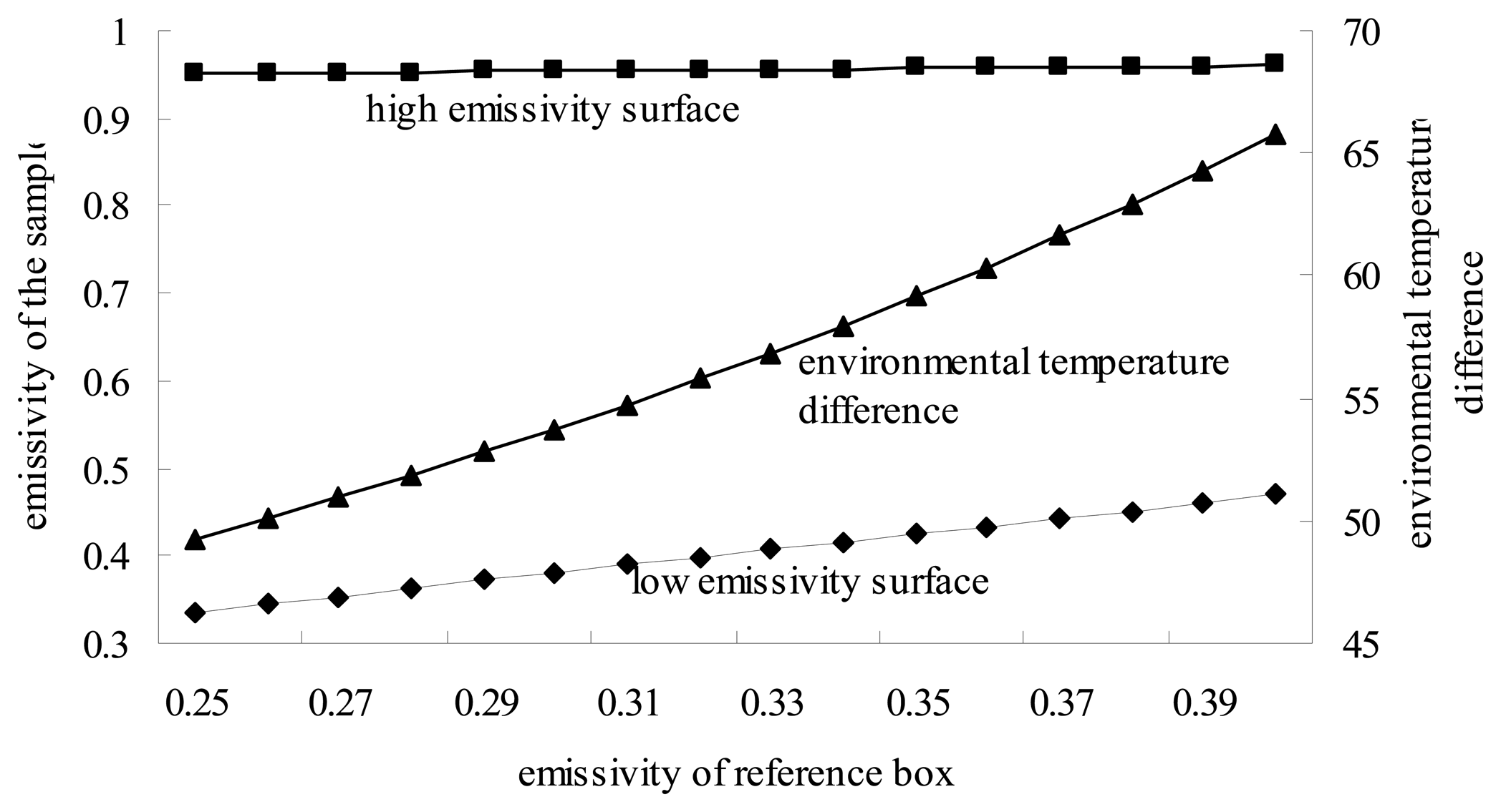
ε_r, the emissivity of reference box. In the calculation of emissivity, ε_r is mainly used to retrieve ambient radiance T_envi, consequently, affects the retrieval of sample's emissivity. Integrating Eq.(2) and Eq.(5) into Eq.(6), we can analyze the relationship between ε_r, T_envi and the emissivity of the sample. Figure.6 shows the simulated results. Clearly, under the conditions that M₁, M₂, M₃, M₄ and T_r are constant, the difference of environmental temperature (T_h–T_c) increases as ε_r increases,accordingly, the calculated emissivities ε_s also increase. For the sample with higher emissivity about 0.95, the results show little change. An variation of 0.01 in ε_r only results in 0.00066 change of ε_s. Comparatively, 0.01variation in ε_r causes 0.0088 change of ε_s for the sample with lower emissivity about 0.33, which is thirteen times than the former case. Therefore, higher attention should be paid when target object of low emissivity is measured and in this case, ε_r should be determined precisely. While in common cases that the samples are soils or vegetations, the effects result from the small error of ε_r can be ignored in the applications. Using the experimental data,

Table 4. Relationship between ε_r and the calculated emissivity.

	Average emissivity
εr	aluminum	vegetation	dry sandy soil	dry agricultural soil	wet sandy soil
0.3	0.285	0.9812	0.940	0.945	0.964
0.32	0.305	0.9815	0.942	0.947	0.965
0.34	0.326	0.9817	0.944	0.949	0.966
0.36	0.346	0.9819	0.945	0.95	0.967
0.38	0.366	0.9822	0.947	0.952	0.968
0.4	0.387	0.9825	0.949	0.953	0.969

was obtained, which exhibited good consistence with the above conclusion, that is to say, ε_r has larger effects on objects of low emissivity.

(4)

T_s, the true temperature of the sample. As the above said, the equation for calculating emissivity (Eq.6) is build on the assumption of T₂ = T₃. Although time difference between the second and the third measurement is very short about 5s, because the temperature of sample and that of the environment are different, there still exists energy exchange between them before reaching the status of energy equilibrium. Thus, T_s2 ≠ T_s3 in reality, and Eq.(6) must be modified to get more correct emissivity. Here, the method for correcting emissivity presented by Zhang (2004) was adopted. More details can be found in that paper. In terms of the method, one additional measurement was taken outside the cloth chamber before the measurement of M₁. The measured radiance was called as M₀, which can be expressed by

$$M_{0,8-14\mu m}(T_0)={\mathit{\varepsilon }}_{s,8-14\mu m}{B}_{8-14\mu m}(T_{s0})+(1-{\mathit{\varepsilon }}_{s,8-14\mu m})B_{8-14\mu m}(T_c)$$

(7)

Using ΔT₂₀ =T_s2 – T_s0 and ΔT₃₀ =T_s3 – T_s0 to describe the change of sample temperature during the period of measurements 0 and 2, and measurements 0 and 3, we obtained the new versions of Eq.(3) and Eq.(4).

$$M_{2,8-14\mu m}(T_2)={\mathit{\varepsilon }}_{s,8-14\mu m}{B}_{8-14\mu m}(T_{s2})+(1-{\mathit{\varepsilon }}_{s,8-14\mu m})B_{8-14\mu m}(T_h)={\mathit{\varepsilon }}_{s,8-14\mu m}{B}_{8-14\mu m}(T_{s0}+\mathrm{\Delta }{T}_{20})+(1-{\mathit{\varepsilon }}_{s,8-14\mu m})B_{s,8-14\mu m}(T_h)$$

(8)

$$M_{3,8-14\mu m}(T_3)={\mathit{\varepsilon }}_{s,8-14\mu m}{B}_{8-14\mu m}(T_{s3})+(1-{\mathit{\varepsilon }}_{s,8-14\mu m})B_{8-14\mu m}(T_c)={\mathit{\varepsilon }}_{s,8-14\mu m}{B}_{8-14\mu m}(T_{s0}+\mathrm{\Delta }{T}_{30})+(1-{\mathit{\varepsilon }}_{s,8-14\mu m})B_{8-14\mu m}(T_c)$$

(9)

Suppose that the durations between the measurements 0 and 2, and 2 and 3 are the same, and the changes of sample surface temperature are approximately identical, i.e. ΔT₂₀ = ΔT₃₂, then ΔT₃₀ ≈ 2ΔT₂₀. Combining Eq.(8) and Eq.(9) with Eq.(7) and eliminating the variables T_s0 and ΔT₂₀, surface emissivity can be calculated from three radiometric measurements by

$${\mathit{\varepsilon }}_{s,8-14\mu m}=1-\frac{M_2-0.5(M_0+M_3)}{B_{8-14\mu m}(T_h)-B_{8-14\mu m}(T_c)}$$

(10)

Table 5. Difference between the uncorrected emissivity calculated by Eq.(6) and the corrected emissivity calculated by Eq.(10).

	Min	Max	Mean	Std
aluminum	0.0	0.0063	0.0019	0.0014
vegetation	0.0	0.0273	0.0035	0.0031
dry sandy soil	0.0	0.0279	0.0032	0.0046
dry agricultural soil	0.0	0.0104	0.0021	0.0017
wet sandy soil	0.0	0.0257	0.0032	0.0030

shows the emissivity difference computed by Eq.(6) and Eq.(10) with our experimental data. So, we can see that the computed emissivity is reduced averagely by 0.0019 – 0.0032 and the maximum is 0.0279 after temperature correction, which suggested that in some cases, the assumption of T₂ = T₃ would induce large errors, but in what conditions it happened, it still need to be explored.

5. Ideal Temperature Difference between Hot Environment and Cool Environment

The above method for calculating emissivity is established on the basis of the series measurements respectively conducted in hot environment and in cool environment. It is by means of the irradiance difference of hot environment and cool environment that the emissivity can be retrieved. However, in the case that the irradiance difference of the two environments is small, it is highly possible that the emissivity can not be obtained due to large signal/noise ratio results from random errors and measurement errors during the measurement. That is to say, there exists a threshold for the irradiance difference of the two environments above which surface emissivity can be retrieved.

Using ΔT=T₂-T₃ to express radiometric temperature difference of the sample measured in hot environment and in cool environment, the following equation can be acquired based on Eq.(3) and Eq.(4).

$$\mathrm{\Delta }T=\sqrt[4]{{\mathit{\varepsilon }}_s{T}_s^4+(1-{\mathit{\varepsilon }}_s)T_h^4}-\sqrt[4]{{\mathit{\varepsilon }}_s{T}_s^4+(1-{\mathit{\varepsilon }}_s)T_c^4}$$

(11)

Because the accuracy of the thermal camera used in the experiment is 0.5k, ΔT ≥ 0.5must be satisfied, and the irradiance difference of the two environments can be observed. In general, sample surface temperature (T_s) is very close to the cool environmental temperature if the sample is put in this environment for enough time, so supposing T_s = T_c, the hot environmental temperature (T_h) can be estimated.

Table 6. Relationship between (T_h-T_c) and ΔT for different ε_s.

εs		Th-Tc
	ΔT=0.5	ΔT =1.0	ΔT =1.5
0.98	22.421	41.036	57.097
0.96	11.814	22.471	32.212
0.94	8.026	15.506	22.522
0.85	3.287	6.486	9.604
0.75	1.985	3.941	5.870
0.45	0.907	1.810	2.710
0.3	0.713	1.425	2.136
0.2	0.624	1.248	1.871
0.07	0.537	1.074	1.612

lists the variation of the estimated environmental temperature difference (T_h-T_c) with ΔT for several samples when T_c equals to 300k. For example, when ε_s= 0.98 and ΔT=0.5, T_h-T_c equals to 22.42, that is, the environmental temperature difference must larger than 22.42, then the emissivity can be calculated using the above method. So we can conclude that when soils or vegetations are observed, in terms of their emissivities (larger than 0.94), environmental temperature difference should be in the range from 8k to 23k, which is easy to be satisfied in clear day of spring and summer.

6. Scaling Effects of Emissivity Retrievals

A common approach to study the effects of resolution between fine and coarse resolution results is to compare data from sensors with varying resolutions or to aggregate fine resolution data to larger cell sizes (Garrigues et al, 2006; Liang, 2000; Chen, 1999; Raffy, 1994). Using our experimental data, scaling effects due to nonlinearity and discontinuous on emissivity retrievals are discussed by means of aggregating fine resolution data to larger cell sizes. Because if the surface emissivity and surface temperature variations are small within a pixel, there are almost no scaling effects (Becker and Li, 1995), in order to increase the emissivity and surface temperature contrast within the pixel and acquire obvious scaling effects, in the experiment, we adopted upper surface of the reference boxes as the sample. By means of pouring hot water into one reference box and pouring cool water into the other reference box, different combinations of emissivity and temperature: high surface emissivity with high temperature, high surface emissivity with low temperature, low surface emissivity with high temperature and low surface emissivity with low temperature, are established. In this way, a whole pixel (coarse resolution) with four sub-pixels (fine resolution) of identical area is constructed, seen from Figure. 2a and will be used to study scaling effects.

Currently, two definitions of coarse resolution emissivity are often used in the applications. For a flat pixel composed by some homogeneous sub-pixels, if sub-pixel information is known, the emissivity for this pixel can be expressed as (Norman and Becker, 1995; Brunsell and Gillies, 2003)

$${\mathit{\varepsilon }}_{c1}=a_1{\mathit{\varepsilon }}_1+a_2{\mathit{\varepsilon }}_2+\cdots =a_1{\mathit{\varepsilon }}_1\frac{B_i(T_1)}{B_i(T_1)}+a_2{\mathit{\varepsilon }}_2\frac{B_i(T_2)}{B_i(T_2)}+\cdots =1-\rho$$

(12)

$${\mathit{\varepsilon }}_{c2}=a_1{\mathit{\varepsilon }}_1\frac{B_i(T_1)}{B_i(T_0)}+a_2{\mathit{\varepsilon }}_2\frac{B_i(T_1)}{B_i(T_0)}+\cdots$$

(13)

where a₁, a₂ … are area proportion of sub-pixel in the whole pixel, a₁ + a₂ + … = 1, ε₁, ε₂, … are emissivities of sub-pixels, T₁, T₂, … are true surface temperature of sub-pixels, ρ is surface reflectivity in thermal wave band. T₀ is a reference temperature for the whole pixel and often take the average value of all sub-pixel temperatures, B_i (T₁), B_i (T₂), … are radiance of black body with temperatures T₁ and T₂ for bandwidth i. Clearly, their only difference is that T₁ and T₂ are replaced by T₀ in the denominator. The following equation quantifies the difference in emissivity retrievals between the two methods.

$$\mathrm{\Delta }\mathit{\varepsilon }={\mathit{\varepsilon }}_{c1}-{\mathit{\varepsilon }}_{c2}=a_1{\mathit{\varepsilon }}_1[1-\frac{B_i(T_1)}{B_i(T_0)}]+a_2{\mathit{\varepsilon }}_2[1-\frac{B_i(T_2)}{B_i(T_0)}]+\cdots$$

(14)

According to Kirchhoff's law, for an opaque surface, ε +ρ=1, so Eq.(12) can be rewritten as

$${\mathit{\varepsilon }}_{c1}=a_1\left(1-{\rho }_1\right)+a_2\left(1-{\rho }_2\right)+\cdots =1-\rho$$

(15)

It should be noted that there is no scaling problem if acquiring coarse resolution emissivity by means of Eq.(12), because essentially, surface emittance or reflectance at coarse resolution is the weighted result of emittance or reflectance of sub-pixels, which is a natural principle. Once ρ is measured, ε can be obtained. Nevertheless, in practice, there is no way to acquire ρ in that the reflection term from atmospheric or environment and surface reflectance are bound together. Therefore, as the above section I mentioned, scaling problem would occur when using some algorithm to retrieve emissivity or temperature. Using Eq.(14), we studied the scaling effects of emissivity.

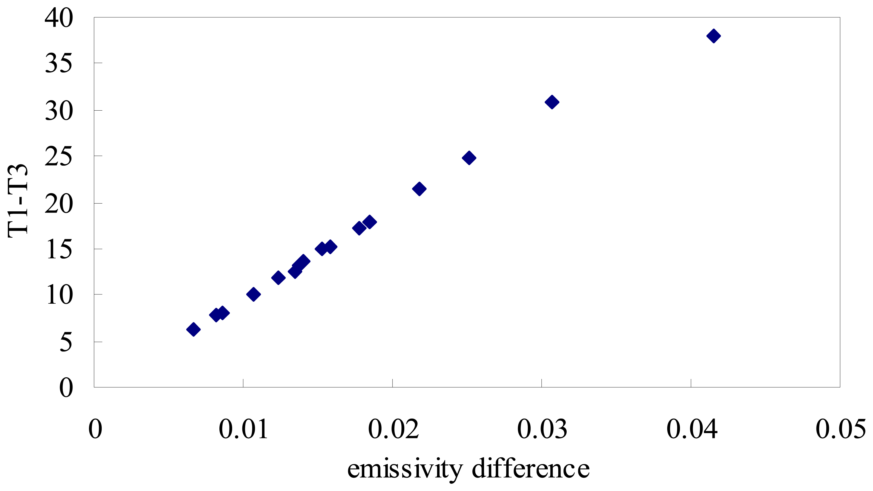
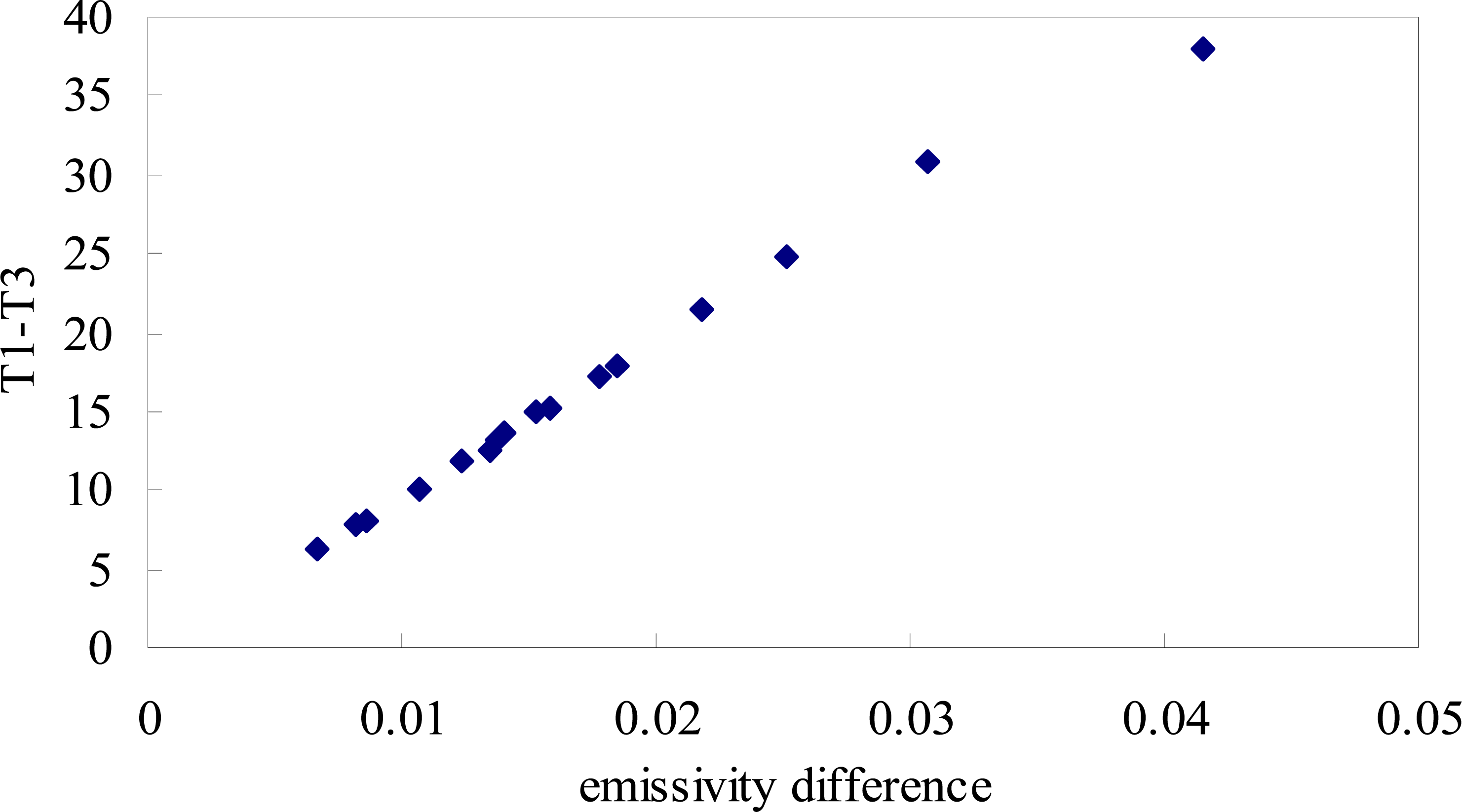
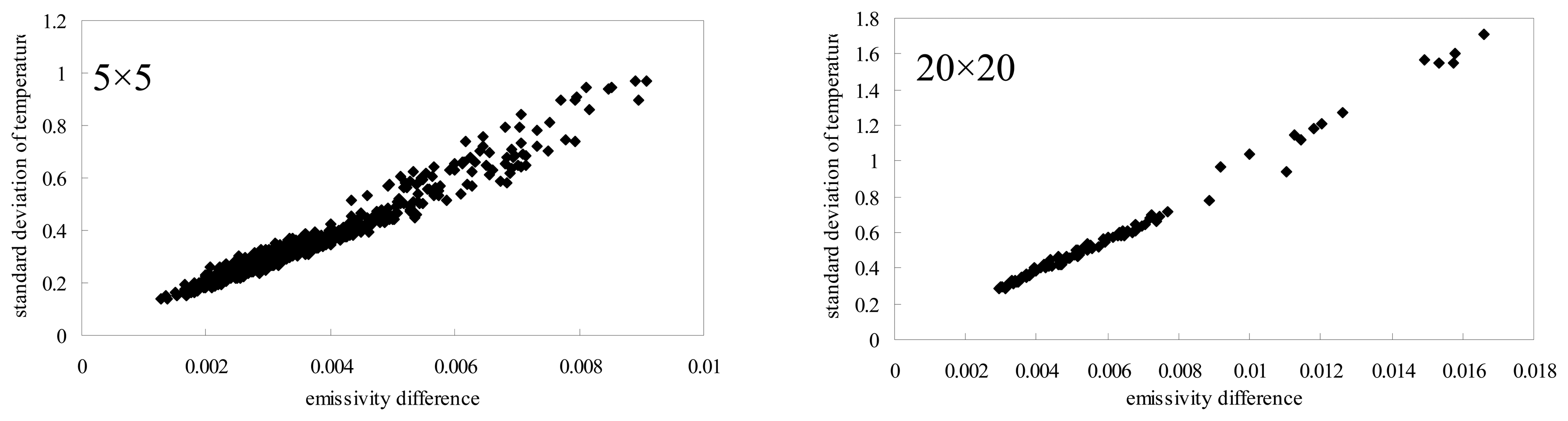
According to the design of reference box, there are four sub-pixels, ε₁=0.3, ε₂=0.98, ε₃=0.3, ε₄=0.98, a₁=a₂= a₃=a₄=0.25, T₁=T₂, T₃=T₄. Calculation results show that the magnitude of Δ ε linearly depends on the temperature difference of sub-pixels (T₁ – T₃). From figure.7, we can see that Δε increases with increase of T₁ – T₃. When T₁ – T₃ equals to 38k, Δ ε can reach 0.04, which will produce large errors in surface temperature retrievals. Furthermore, using the emissivity retrievals of combinations of soils and vegetations, we obtained the similar linear results. There are total 240×180 pixels in a thermal image, correspondingly, there are 240×180 surface emissivity values. By integrating pixels of 5×5, 20×20, respectively, we obtained figure.8a and figure.8b, where we used standard deviation of surface temperatures to express the heterogeneity of measured objects. Clearly, the more heterogeneity of the surface is, the larger emissivity difference is. 1.0 deviation of temperature results in about 0.01 emissivity difference. Therefore, Δε must be evaluated and be corrected to fulfill the emissivity scaling.

7. Summary and Conclusions

For measuring spatial distribution of surface emissivty and studying scaling effects of it, at same time, providing theoretical and practical foundations for the implement of measuring surface emissivty on airborne or spaceborne, an automatic instument for studying scaling effects of emissivity is designed, with which, the emissivity of various samples has been measured and the sensitivities of four important factors to emissivity calculation: M, the measured apparent radiance; T_envi, environmental temperature; ε_r, the emissivity of reference box; T_s, the true temperature of the sample, have been analyzed. It showed that for the sample of low emissivity, small variances of T_envi and ε_r would cause large changes in calculated emissivity, therefore, in such cases, more attentions should be paid. Whereas, for the sample of high emissivity (higher than 0.9), the magnitude of variances caused by T_envi and ε_r is about 10^-3, which often can be ignored in common applications. By means of taking additional measurement outside the cloth chamber, the errors caused by the change of sample's temperature itself was estimated and corrected. According to our experimental data, in some cases, large errors can be generated. At last, the analysis about the effects of resolution on emissivity results showed that emissivity difference linearly depends on the temperature difference of sub-pixels and the more heterogeneity of the surface is, the larger emissivity difference is. Therefore, for the surface of high heterogeneity, emissivity difference must be evaluated and be corrected to fulfill the emissivity scaling.

References and Notes

- Buettner, C.D.; Kern, K.J.K. The determination of infrared of emissivities of terrestrial surface. Journal of Geophysical Research 1965, 70, 1327–1337. [Google Scholar]
- Barducci, A.; Pippi, I. Temperature and emissivity retrieval from remotely sensed images using the “grey body emissivity” method. IEEE Trans. Geosci. Remote Sens 1996, 34, 681–695. [Google Scholar]
- Becker, F. The impact of spectral emissivity on the measurement of land surface temperature from a satellite. International Journal of Remote Sensing 1987, 10, 1509–1522. [Google Scholar]
- Becker, F.; Li, Z.L. Temperature-independent spectral indices in thermal infrared bands. Remote Sensing of Environment 1990, 32, 17–33. [Google Scholar]
- Becker, F.; Li, Z.L. Surface temperature and emissivity at various scales: definition measurement and related problems. Remote Sensing Reviews 1995, 12, 225–253. [Google Scholar]
- Brunsell, N.A.; Gillies, R.R. Length scale analysis of surface energy fluxes derived from remote sensing. Journal of Hydrometeorology 2003, 4, 1212–1259. [Google Scholar]
- Coll, C.; et al. On the Atmospheric Dependence of the Split-Window Equation for Land-Surface Temperature. Int J Remote Sens 1994, 15, 105–122. [Google Scholar]
- Gillespie, A.R.; Rokugawa, S.; Matsunaga, T.; Gothern, J.S.; Hook, S.; Kahle, A.B. A temperature and emissivity separation algorithm for advanced spaceborne thermal emission and reflection radiometer (ASTER) images. IEEE Trans. Geosci. Remote Sens 1998, 36, 1113–1126. [Google Scholar]
- Li, X.W.; Strahler, A.; Fried, M. A conceptual model for effective directional emissivity for non isothermal surface. IEEE Trans. Geosci. Remote Sens 1999, 37, 2508–2517. [Google Scholar]
- Li, Z.L.; Becker, F.; Stoll, M.P.; Wan, Z.M. Evaluation of six methods for extracting relative emissivity spectral from thermal infrared images. Remote Sensing of Environment 1999, 69, 197–214. [Google Scholar]
- Liu, Y.B.; Hiyama, T.; Yamaguchi, Y. Scaling of land surface temperature using satellite data: A case examination on ASTER and MODIS products over a heterogeneous terrain area. Remote Sensing of Environment 2006, 105, 115–128. [Google Scholar]
- Moran, M.S.; Humes, K.S.; Printer, P.J., Jr. The scaling characteristics of remotely sensed variables for sparsely-vegetated heterogeneous landscapes. Journal of Hydrology 1997, 190, 337–362. [Google Scholar]
- Nerry, F.; Labed, J.; Stoll, M.P. Emissivity signatures in the thermal infrared band for remote sensing: calibration procedure and method of measurement. Applied Optics 1988, 27, 758–764. [Google Scholar]
- Nerry, F.; Labed, J.; Stoll, M.P. Spectral properties of land surfaces in the thermal infrared 1. Laborataory measurements of absolute spectral emissivity signatures. Journal of Geophysical Research 1990, 95, 7027–7043. [Google Scholar]
- Nerry, F.; Stoll, M.P.; Kologo, N. Scattering of a CO2 laser beam at 10.6um by bare soils: experimental study of the polarized bidirectional scattering coefficient; model and comparison with directional emissivity measurements. Applied Optics 1991, 30, 3984–3994. [Google Scholar]
- Norman, J.M.; Becker, F. Terminology in thermal infrared remote sensing of natural surface. Agriculture and Forest Meteorology 1995, 77, 153–176. [Google Scholar]
- Qin, Z.H.; et al. Derivation of split window algorithm and its sensitivity analysis for retrieving land surface temperature from NOAA-advanced very high resolution radiometer data. J Geophys Res-Atmos 2001, 106, 22655–22670. [Google Scholar]
- Rivard, B.; Thomas, P.J.; Giroux, J. Precise emissivity of rock samples. Remote Sensing of Environment 1995, 54, 152–160. [Google Scholar]
- Rubio, E.; Caselles, V.; Badenas, C. Emissivity Measurements of Several Soils and Vegetation Types in the 8-14μm Wave Band: Analysis of Two Field Methods. Remote Sensing of Environment 1997, 59, 490–521. [Google Scholar]
- Sobrino, J.A.; Caselles, V. A field method for estimating the thermal infrared emissivity. ISPRS Journal of Photogrammetry and Remote Sensing 1993, 48, 24–31. [Google Scholar]
- Su, H.B.; et al. Thermal model for discrete vegetation and its solution on pixel scale using computer graphics. Sci. China Ser. E 2000a, 43, 48–54. [Google Scholar]
- Su, H.B.; et al. Determination of the effective emissivity for the regular and irregular cavities using Monte-Carlo method. Int. J. Remote Sens 2000b, 21, 2313–2319. [Google Scholar]
- Su, H.B.; et al. Modeling evapotranspiration during SMACEX: Comparing two approaches for local- and regional-scale prediction. J. Hydrometeorol 2005, 6, 910–922. [Google Scholar]
- Su, H.; et al. Evaluation of remotely sensed evapotranspiration over the CEOP EOP-1 reference sites. J. Meteorol. Soc. Jpn 2007, 85A, 439–459. [Google Scholar]
- Wan, Z.M.; Li, Z.L. A physics-based algorithm for retrieving land-surface emissivity and temperature from EOS/MODIS data. IEEE Trans. Geosci. Remote Sens 1997, 35, 980–996. [Google Scholar]
- Wan, Z.M.; Zhang, Y.; Zhang, Q.; Li, Z.L. Validation of the land-surface temperature products retrieved from Terra Moderate Resolution Imaging Spectroradiometer data. Remote Sensing of Environment 2002, 83, 163–180. [Google Scholar]
- Watson, K. Two-temperature method for measuring emissivity. Remote Sensing of Environment 1992a, 42, 117–121. [Google Scholar]
- Zhang, R.H. A proposed approach to determine the infrared emissivities of terrestrial surfaces from airborne or spaceborne platforms. International Journal of Remote Sensing 1989, 3, 591–595. [Google Scholar]
- Zhang, R.H.; Li, Z.L.; Tang, X.Z.; Sun, X.M.; Su, H.B.; Zhu, Z.L. Study of Emissivity Scaling and Relativity of Homogeneity of Surface Temperature. International Journal of Remote Sensing 2004, 25, 245–259. [Google Scholar]
Figure 1.
An automatic instrument to measure environmental radiation and component emissivity. (a) cool environment; (b) hot environment
Figure 2.
Picture of reference boxes: a) upper surface; b) undersurface.
Figure 3.
Picture of the sample plate.
Figure 4.
Distribution image of emissivities.
Figure 5.
Error distribution in view field of thermal camera.
Figure 6.
Effects of εr on the calculated emissivity.
Figure 7.
Relationship between Δε and (T1 – T3).
Figure 8.
Relationship between Δ ε and standard deviation of surface temperatures.