Article

Improving Distributed Runoff Prediction in Urbanized Catchments with Remote Sensing based Estimates of Impervious Surface Cover

1
Warsaw Agricultural University, Department of Hydraulic Structures and Environmental Restoration, Warsaw, Poland
2
Vrije Universiteit Brussel, Cartography and GIS Research Unit, Department of Geography, Brussels, Belgium
3
Vrije Universiteit Brussel, Department of Hydrology and Hydraulic Engineering, Brussels, Belgium
4
K.U.Leuven, Department of Earth and Environmental Sciences, Heverlee, Belgium
*
Author to whom correspondence should be addressed.
Sensors 2008, 8(2), 910-932; https://doi.org/10.3390/s8020910
Submission received: 15 January 2008 / Accepted: 7 February 2008 / Published: 15 February 2008
(This article belongs to the Special Issue Remote Sensing of Natural Resources and the Environment)

Abstract

:
The amount and intensity of runoff on catchment scale are strongly determined by the presence of impervious land-cover types, which are the predominant cover types in urbanized areas. This paper examines the impact of different methods for estimating impervious surface cover on the prediction of peak discharges, as determined by a fully distributed rainfall-runoff model (WetSpa), for the upper part of the Woluwe River catchment in the southeastern part of Brussels. The study shows that detailed information on the spatial distribution of impervious surfaces, as obtained from remotely sensed data, produces substantially different estimates of peak discharges than traditional approaches based on expert judgment of average imperviousness for different types of urban land use. The study also demonstrates that sub-pixel estimation of imperviousness may be a useful alternative for more expensive high-resolution mapping for rainfall-runoff modelling at catchment scale.

1. Introduction

Remote sensing and GIS technology is increasingly integrated with hydrological modelling. Digital elevation models (DEMs), digital data of soil type and land use, as well as powerful GIS tools have opened new possibilities for hydrological research leading to a more data driven modelling and understanding of the fundamental physical processes underlying the hydrological cycle. Recently, many hydrological models with a flood prediction component have been developed or have been updated to use DEMs, such as SWAT [1], CASC2D [2], DWSM [3], HYDROTEL [4], whereas models like SHE and TOPMODEL were adapted to benefit from GIS data [5, 6]. These models are either loosely or tightly coupled with GIS and remotely sensed data.
Remote sensing techniques have the ability to provide spatial and temporal information of the land surface, which is needed for parameterization of distributed hydrological models. In general, remote sensing data are used for hydrological modelling in the following ways: (1) to quantify surface parameters, such as land-cover type and density [4, 7] or surface roughness [8, 9]; (2) to identify hydrologically significant areal phenomena for spatial model output verification, such as flooded areas [10-12] and snow cover [13, 14]; (3) to produce field representations of hydrologically important parameters, such as soil moisture and leaf area index (LAI), used for calculation of interception and evapotranspiration, and thus the water balance of a watershed [15-18].
One of the most important inputs for spatially distributed rainfall-runoff models, particularly in urbanized areas, is the amount and distribution of sealed surfaces. The presence of anthropogenic impervious surfaces in urbanized areas leads to more surface runoff, which in turn increases the risk for water pollution and floods in the watershed, hampers the recharge of aquifers and boosts erosion [19, 20]. Furthermore, impervious surfaces are warmer than their natural surroundings. This may have a profound impact on the local climate and the temperature of surface water. Information on the spatial distribution of impervious surfaces is therefore important in hydrological modeling and is also increasingly used as a key indicator for the ecological condition of a watershed [20, 21].
Different methods have been proposed for impervious surface mapping, many of which rely on existing land-use data sets [21-23]. These so-called indirect methods associate a percentage of imperviousness with each land-use type. The drawback of this approach is that there is no standardized method for deriving these estimates and that there may be a high variability in the amount of imperviousness within the same land-use class. If mapping at a spatially more detailed level is required, a direct approach is preferred. Field inventorying and visual interpretation of large-scale, ortho-rectified aerial photographs are the most reliable methods to map impervious surfaces. However, because these methods are very time-consuming, they can in practice only be applied to relatively small areas. Satellite imagery, obtained from high-resolution sensors like Ikonos or Quickbird, offers an interesting alternative for producing maps of surface imperviousness. Although high-resolution imagery may not provide the same level of detail as large-scale aerial photographs, the use of automated or semi-automated image interpretation methods, exploiting the multi-spectral information content of the imagery, substantially reduces the effort that is required to produce reliable information on the distribution of impervious surfaces.
Despite the advantages of deriving impervious surface maps directly from high-resolution satellite imagery, the relatively limited footprint and the cost of such images pose difficulties if impervious surface maps are required for larger areas. A less expensive and more efficient alternative to map the spatial distribution of imperviousness in such cases is to develop models that allow estimation of the degree of imperviousness inside medium-resolution image pixels (Landsat ETM+, ASTER,…). Over the past years, many sub-pixel regression methods and sub-pixel classification methods have been proposed to derive the proportion of impervious surfaces within a medium-resolution pixel directly from the available multi-spectral data: multiple regression [24], linear spectral unmixing [25-28], neural networks [29, 30] and decision trees [31-33]. Although the sub-pixel approach does not allow one to achieve the same degree of accuracy as when high-resolution data would be used, most studies report an average per pixel proportional error in the estimation of impervious surfaces of close to 10 %.
In this study, multiple layer perceptron (MLP) models were used for mapping the proportion of four major land-cover classes (impervious surfaces, vegetation, bare soil and water/shade), using both high-resolution and medium-resolution satellite data. First a detailed land-cover map was produced by classifying a 4-meter resolution multi-spectral Ikonos image covering part of the city centre and the south-eastern suburbs of Brussels and the adjacent Sonian Forest. The high-resolution land-cover map was then used to train a sub-pixel classification model that estimates surface cover proportions within the pixels of a medium-resolution image (Landsat ETM+) covering the entire Brussels agglomeration. Land-cover class proportions derived from both the high-resolution classification and the medium-resolution sub-pixel classification were used to characterize the distribution of land cover within the urban classes of an existing land-use map, produced by the Flemish Government, and used by regional and local authorities and research institutions within the region. The “remote sensing enhanced” versions of the land-use map were used as input for a rainfall-runoff simulation for the upper part of the Woluwe River catchment, located in the southeastern part of Brussels. The effect of different methods for characterizing urban land cover on estimated peak discharges was examined. Also the results obtained with high-resolution and medium-resolution land-cover data were compared.

2. Study area and data
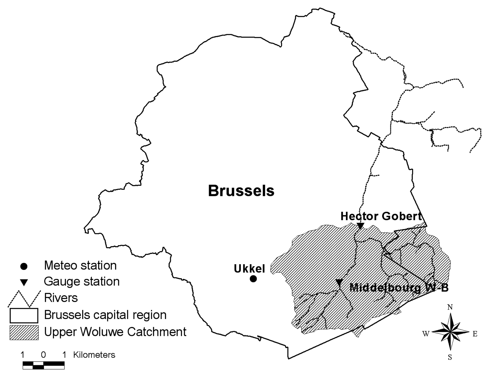
2.1. Study area

The Woluwe is a small river that is part of the Scheldt basin. The upper part of the Woluwe catchment up to the Goubert gauge was selected as a study area (Figure 1). The upstream part of this area lies in the protected zone of the Sonian forest. In the downstream part, the Woluwe River flows partially through several vaulted stretches and park and pond systems. The Upper Woluwe catchment comprises approximately 31 km2. The elevation of the catchment ranges from 49 m to 129 m, with an average of 94 m above sea level. Elevation increases gradually from the north to the south, with slopes varying between 0 and 22 %, with an average of 6 %. According to the Royal Meteorological Institute at Ukkel, located close to the catchment border (Figure 1), the long-term yearly precipitation is 780 mm/year, 380 mm in the winter and 400 mm in the summer. The long-term open-water potential evaporation of Ukkel is 657 mm/year, the winter evaporation is 114 mm, the summer evaporation 543 mm. The average temperature is 5.0°C for the winter season and 14.1°C for the summer season. The Woluwe catchment consists for 96 % of the area of loam soils, while the remaining 4 % are occupied by sandy loam soils.

2.2. Remote sensing data

Two image data sets were used in this study: one of high resolution (Ikonos) to derive a detailed high-resolution land-cover map, and one of medium resolution (Landsat ETM+) for estimating land-cover class proportions at sub-pixel level. The Ikonos image (4 m resolution multi-spectral, 1 m resolution panchromatic) was acquired on June 8th 2000. It covers a large part of the city of Brussels, from the centre towards the south-east. The image was ortho-rectified with an existing digital surface model and put in the Belgian Lambert coordinate system. The medium-resolution data set that was used in the study is a subset (1164 by 1164 pixels) of a Landsat ETM+ (level 1G) image acquired on October 18th 1999 (path 198, row 25). The subset covers the entire city and a good part of its surroundings, including the Upper Woluwe study area described above. It was geometrically co-registered to the Ikonos image by a first-order polynomial transformation. The RMS error on an independent set of control points was 5.78 m, which implies that on the average the geometric shift in x and y between Ikonos and ETM+ data corresponds to less than 4 % of the area of an ETM+ pixel.

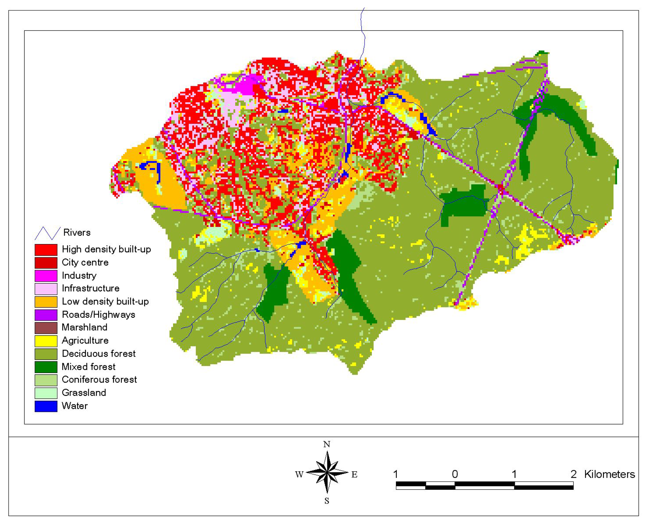
2.3. Land-use, DEM and soil data

The land-use map of Flanders, produced by the Agency for Geographic Information Flanders (AGIV), was used as a reference data set to characterize land use within the study area. The map distinguishes 13 land-use types and was obtained using a hybrid approach combining interpretation of Landsat TM data with existing vector data sets (topographic maps, waterways, soil type, CORINE land-use data) for improvement of the original interpretation and for increasing the number of thematic classes. Dominant land-use types in the study area (Figure 2) are deciduous forest (55 %), urban area (29 %), coniferous forest (4 %) and mixed forest (6 %). Agriculture, grassland, marshland and open water cover 6 % of the total area. The urban part of the study area includes high density built-up area (12.7 %), low density built-up area (8.2 %), infrastructure (5.6 %), roads and highways (1.9 %), industrial land use (0.5 %), and also covers a very small part of the city centre (0.2 %). The original land-use map has a resolution of 20 m. For modeling purposes it was resampled to the 30 m cell size of the Landsat ETM+ data. A DEM with 30 m resolution was constructed from elevation contours and the river network. The elevation contours for every 2.5 m and the river network were digitized from topographic maps at a scale of 1:10,000. The DEM was generated in ArcInfo using TOPOGRID [34]. A digital soil map of the study area was obtained from AGIV and converted into 12 USDA soil texture classes based on textural properties.

2.4. Hydrometeorological data

Rainfall data with 10-minutes time interval and daily potential evapotranspiration (PET) data were obtained from the Ukkel meteorological station for April and May 2005. No continuous discharge data for this period is available for the Hector Goubert station. For the purpose of modelling, the hydrometeorological data were transformed to an hourly time step.

3. Methods

3.1. Hydrological modelling

For rainfall-runoff simulation use was made of WetSpa, a grid-based distributed hydrological model for water and energy transfer between soil, plants and atmosphere, which was originally developed by Wang et al. [35] and adopted for flood prediction by De Smedt et al. [36], and Liu et al. [37]. For each grid cell a vegetation, root, transmission and saturated zone is considered in the vertical direction. The hydrological processes parameterized in the model are: precipitation, interception, depression storage, surface runoff, infiltration, evapotranspiration, percolation, interflow and groundwater flow. The total water balance for a raster cell is composed of the water balance for the vegetated, bare soil, water and impervious parts of each cell. This allows accounting for within-cell heterogeneity of land cover. A mixture of physical and empirical relationships is used to describe the hydrological processes in the model. Interception reduces the precipitation to net precipitation, which on the ground is separated into rainfall excess and infiltration. Rainfall excess is calculated using a moisture-related modified rational method with a potential runoff coefficient depending on land cover, soil type, slope, rainfall intensity, and antecedent moisture content of the soil. The calculated rainfall excess fills the depression storage at the initial stage and runs off the land surface simultaneously as overland flow [38]. The infiltrated part of the rainfall stays as soil moisture in the root zone, moves laterally as interflow or percolates as groundwater recharge depending on the moisture content of the soil. Both percolation and interflow are assumed to be gravity driven in the model. Percolation out of the root zone is determined by the hydraulic conductivity, which is dependent on the moisture content as a function of the soil pore size distribution index. Interflow is assumed to occur in the root zone after percolation and becomes significant only if the soil moisture is higher than field capacity. Darcy's law and a kinematic approximation are used to estimate the amount of interflow generated from each cell, in function of hydraulic conductivity, moisture content, slope, and root depth. The actual evapotranspiration from soil and plants is calculated for each grid cell using the relationship developed by Thornthwaite and Mather [39] as a function of potential evapotranspiration, vegetation stage, and moisture content in the cell.
Runoff from different cells in the watershed is routed to the watershed outlet depending on flow velocity and wave damping coefficient by using the diffusive wave approximation method. An approximate solution proposed by De Smedt et al. [36] in the form of an instantaneous unit hydrograph (IUH) was used in the model, relating the discharge at the end of a flow path to the available runoff at the start of the flow path:
U ( t ) = 1 σ 2 π t 3 / t 0 3 exp [ ( t t 0 ) 2 2 σ 2 t / t 0 ]
where t [T] is time, U(t) [T−1] is the flow path unit response function, t0 [T] is the mean flow time, and σ [T] is the standard deviation of the flow time. Parameters t0 and σ are spatially distributed, and can be obtained by integration along the topographically determined flow paths as a function of flow celerity and dispersion. Although the spatial variability of land use, soil and topographic properties within a watershed are considered in the model, the groundwater response is modelled on sub-catchment scale. The simple concept of a linear reservoir is used to estimate groundwater discharge, while a non-linear reservoir method is optional in the model [40]. The groundwater outflow is added to the generated runoff to produce the total stream flow at the sub-watershed outlet. Time-dependent inputs of the model are precipitation and potential evapotranspiration. Model parameters such as interception and depression storage capacity, potential runoff coefficient, overland roughness coefficient, root depth, soil property parameters, average travel time to the outlet, dispersion coefficient, etc., are determined for each grid cell using lookup tables and a high-resolution DEM, soil type and land-use maps. The main outputs of the model are river flow hydrographs, which can be defined for any location along the channel network, and spatially distributed hydrological characteristics, such as soil moisture, infiltration rates, groundwater recharge, surface water retention, runoff, etc.

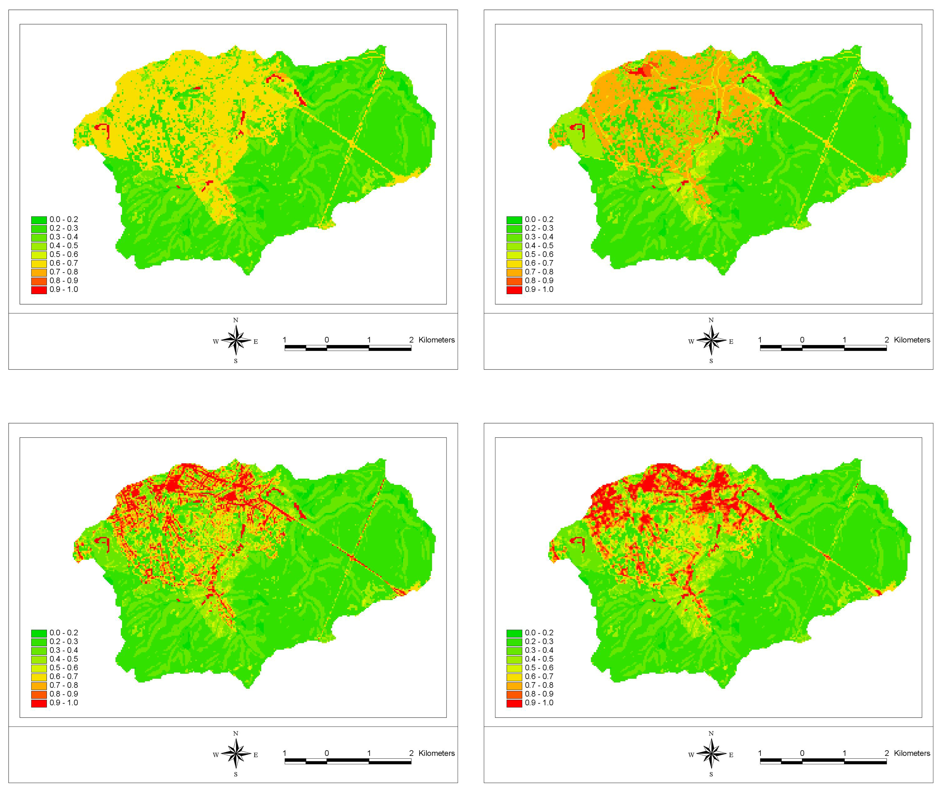
3.2. Estimation of impervious surface cover

In this study, a multi-resolution approach was adopted for detailed mapping of impervious surface cover. First, a high-resolution land-cover map was produced from the Ikonos image covering the study area using a non-parametric multi-spectral classification approach, followed by a procedure for post-classification accuracy improvement. The high-resolution land-cover classification was then used to train a sub-pixel classification model to estimate sub-pixel fractions of four major land-cover classes (vegetation, impervious surfaces, water and bare soil) within a subset of the medium-resolution Landsat ETM+ image overlapping the Ikonos data set.

3.2.1. High-resolution land-cover mapping

To produce a high-resolution land-cover map of the study area, the orthorectified Ikonos image of June 8, 2000 covering the southeastern part of Brussels was used. Applying a multiple layer perceptron classification model built in NeuralWorks Predict®, 10 land-cover classes were distinguished: light and dark red surfaces, light, medium and dark grey surfaces, bare soil, water, crops, shrub and trees, grass. Shadow was added as a separate image class. The class “red surfaces” represents building materials of these colours such as red-tiled squares or parking spaces and roof tiles made of red clay. The “grey surfaces” class is an aggregation of several urban materials with a grey appearance such as concrete, asphalt, slate, etc. Both the “red surfaces” and “grey surfaces” classes were spectrally further divided according to brightness in respectively three and two subclasses to reduce within-class heterogeneity and to improve classification performance. Training data for the classification were obtained by randomly sampling 200 training samples for each class, yielding 2200 training samples in total.
Different classification scenarios were tested, using various combinations of input variables: only the multi-spectral bands, the multi-spectral bands with the PAN band, the multi-spectral bands with the PAN band and a vegetation index (NDVI), and the multi-spectral bands with PAN, NDVI and 2 texture measures: local variance and binary comparison matrix [41]. Best results were obtained with the latter approach. Transformations of the input bands and selection of input features according to their relative contribution to the overall information content were accomplished with NeuralWorks Predict®. The transformed input variables that were retained to actually perform the classification were chosen from a set of 5 mathematical transformations per original input band using a genetic-based variable selection algorithm embedded in the software. The accuracy and the spatial coherence of the classification result was further improved by applying post-classification techniques to remove shadow, reduce structural noise and correct for classification errors. For more details on the post-classification techniques applied the reader is referred to Van de Voorde et al. [42].

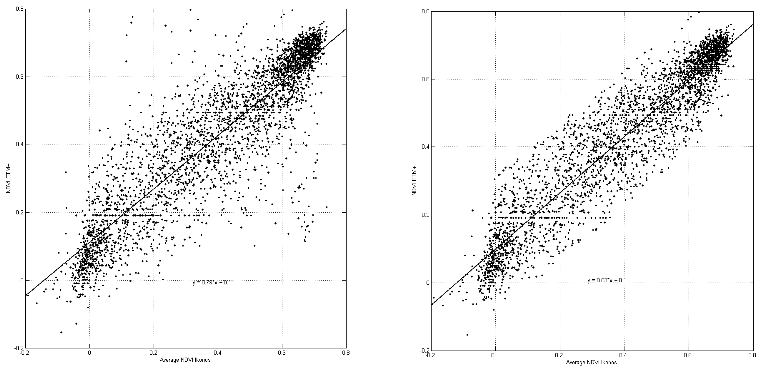
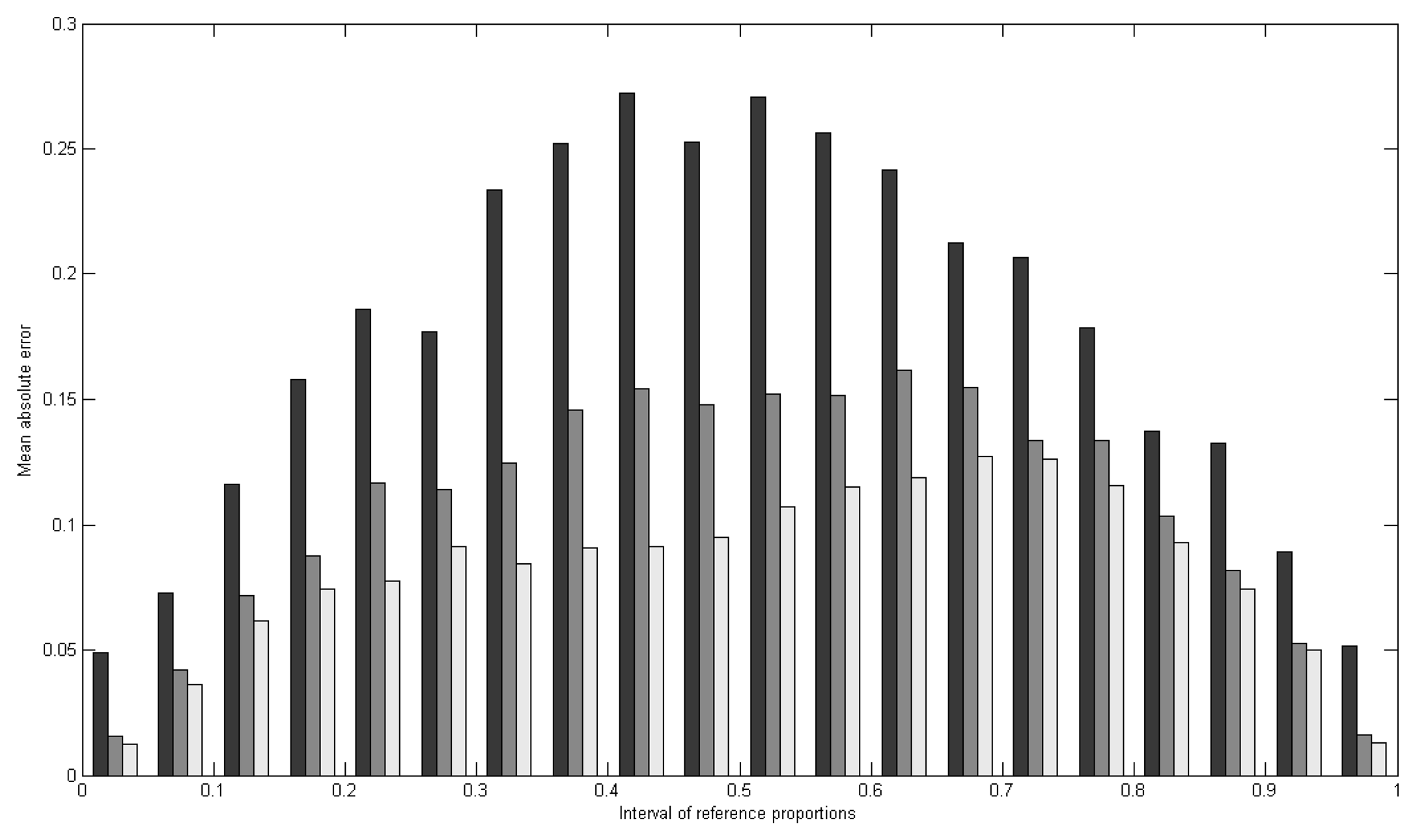
3.2.2. Subpixel classification of Landsat ETM+ imagery

A multiple-layer perceptron approach for sub-pixel classification was adopted to estimate the proportions of four major land-cover classes (impervious surfaces, vegetation, water and bare soil) in each pixel of the Landsat ETM+ image subset. To train the sub-pixel classifier, the 10 classes in the land-cover map derived from the Ikonos image were regrouped into a single vegetation class (including shrub and trees, grass and crops), a single impervious class (including red and grey surfaces), water and bare soil. The map obtained was spatially aggregated to produce reference proportions for the four major land-cover classes for each 30 m resolution ETM+ pixel in the overlapping zone between the two images.
Because the images are not of the same date, precautions had to be taken not to include pixels in the training and validation phase with different land cover in both images due to seasonal shifts (leaf condition, crop cycles,…) or due to a change in land use (e.g. transition from non-built to built area). Since urban areas are dominated by impervious surfaces and vegetation, most changes in the 8-month period between the acquisition dates of both images are expected to be related to changes in the vegetation component of the pixels. Therefore, in order to detect anomalous pixels the ETM+ NDVI values of all pixels in the overlap with the Ikonos image were plotted against the mean NDVI value of the constituent Ikonos pixels, after converting the raw DNs for both images to at-satellite reflectance values using the equations proposed by Taylor [43] and Irish [44]. A strong linear relationship was observed between ETM+ NDVI values and Ikonos mean NDVI values. Pixels deviating significantly from the trend were considered as indicative of major changes in land cover and were not used for training and validation of the sub-pixel classifier.
Feature selection and building of a multiple layer perceptron model for sub-pixel classification were accomplished with NeuralWorks Predict® software, starting from a set of transformations of all multispectral bands (1-5, 7) and all possible ratios between these bands. The performance of the sub-pixel classifier was assessed on an independent validation set by calculating per-class mean error (MECj) and per-class mean absolute error (MAECj):
M E C j = i = 1 N ( P i j P i j ) N
M A E C j = i = 1 N | P i j P i j | N
with:
  • N: the total number of pixels in the validation sample
  • Cj: target class j
  • Pij: the proportion of class j inside validation pixel i, derived from the high-resolution land-cover map (ground truth)
  • P′ij: the proportion of class j inside validation pixel i, estimated by the sub-pixel classifier
The per-class mean error MECj gives an indication of possible bias in the estimation of proportions (over or underestimation). The per-class mean absolute error MAECj quantifies the amount of error and can be interpreted as a mean error percentage. To assess the impact of cell aggregation on proportional accuracy, all error measures were calculated at the original 30 m resolution, as well as after aggregation of proportions to 60 m and 90 m.

3.3. Formulation of scenarios

Using high-resolution or medium-resolution land-cover information derived from satellite imagery, land-use maps of urbanized areas can be improved by estimating an average percentage of imperviousness for the urban area as a whole (scenario 1); an average percentage of imperviousness for different types of urban land use (scenario 2); a local percentage of imperviousness for every individual cell within the urban area (scenario 3). The three scenarios, corresponding to a gradual increase of information on the spatial distribution of imperviousness, were tested in this study, by combining high-resolution and medium-resolution estimates of land-cover imperviousness with information on the distribution of various types of urban land use provided by the land-use map of Flanders. The effect of the three scenarios on the estimation of peak discharges was evaluated. Also the effect of using medium-resolution instead of high-resolution estimates of imperviousness on the outcome of the rainfall-runoff modeling was examined.

3.3.1. Scenario 1: Homogeneous distribution of impervious surfaces (non-distributed approach)

This scenario assumes a homogeneous distribution of impervious surfaces for the whole urban area. It simulates a situation, which regularly occurs in hydrology in practice, i.e. neither is there information available about different types of urban land use, nor about different levels of imperviousness within the urban area. To simulate runoff for this scenario the various urban land-use classes in the Flemish land-use map were aggregated into a single urban class. The WetSpa default land-cover parameter values define an urban class as composed of 30 % sealed surfaces, with the remaining area covered by grass. For this combination the surface runoff coefficient and depression storage were calculated as a weighted average [45]. This basic scenario was improved by using the 30 m resolution estimates of imperviousness, derived from the Ikonos land-cover map and from the ETM+ sub-pixel classification to estimate the average percentage of imperviousness for urban area in a less arbitrary way.

3.3.2. Scenario 2: Land-use specific distribution of impervious surfaces (semi-distributed approach)

In this scenario, each type of urban land use is assigned a different level of imperviousness. As explained earlier, the land-use map of Flanders distinguishes 6 types of urban land use. Initially three levels of imperviousness were assumed: 30 % for low density built-up area, 50 % for infrastructure, high-density built-up area, roads and highways, and 70 % for the city centre and for industrial areas [46]. The remaining of the urban cells was considered as covered by grass. Consequently the surface runoff coefficient and depression storage is calculated as a weighted average. Then the semi-distributed scenario was improved by extracting an average percentage of imperviousness for the different urban land-use classes from the Ikonos-derived land-cover map and, secondly, from the ETM+ sub-pixel proportion of impervious surfaces map.

3.3.3. Scenario 3: Cell-specific distribution of impervious surfaces (fully-distributed approach)

In this scenario local variations in the level of imperviousness within each urban land-use type are taken into account. This time the land cover in every urban land-use cell is described as consisting of four major cover types (vegetation, impervious, water and bare soil), of which the proportion is obtained from the high-resolution and medium-resolution remotely sensed imagery. The runoff coefficient and depression storage for each cell are then estimated as an area weighted average of the parameters for vegetation, impervious surfaces, water and bare soil.

4. Results and discussion

4.1. Estimation of impervious surface cover

4.1.1. High-resolution land-cover mapping

The pixel-based classification of the Ikonos image was obtained by training and comparing several multiple layer perceptron models, using different combinations of input bands. The best performing network consisted of 9 inputs, 17 hidden nodes and 11 output nodes (i.e. the 11 image classes). The input variables used were mathematical transformations of the red, green and blue image bands, the NDVI and two texture measures, namely standard deviation and binary comparison matrix. After classification, the two red surface classes (light, dark) and the three grey surface classes (light, medium, dark) were aggregated into one red surface class and one grey surface class respectively, reducing the total number of classes to 7 + shadow. The overall performance of this network on an independent set of validation pixels was characterized by a kappa index-of-agreement of 0.91.
Despite the relatively high numeric accuracy of the classification result, many problems such as shadow, structural clutter and classification errors remained. The first step in improving the classification was to remove the shadow pixels using a technique described in Van de Voorde et al. [42]. In this approach, pixels originally classified as shadow are assigned to the most likely land-cover class using a second multiple layer perceptron (MLP) model. This neural network models the relationship between the class activation levels assigned to the shadow pixel by the initial MLP and the actual type of land cover present beneath the shadow, based on a set of shadow training pixels for which the type of land cover is known [42]. The second step of the post-classification enhancement consisted of applying knowledge-based rules to correct classification errors and to reduce structural clutter, based on contextual information. In total, 14 region-based rules were developed and applied to the land-cover classification after shadow removal [47]. Post-classification improvement of the land-cover map increased the kappa index from 0.91 to 0.95 (Table 1). Apart from the confusion between grass and crops the accuracy of the land-cover map is high. The relatively low producer's accuracy for crops is mostly due to the erroneous commission of cropland to meadow. This confusion mainly occurs in the rural area surrounding the Brussels region. It does not occur in the urbanized area of the Woluwe catchment and, as such, it did not have an impact on the results of the runoff modeling in this study.
The 7 classes in the land-cover map were grouped into four major land-cover classes (vegetation, impervious surfaces, water and bare soil). Finally, the resulting map was spatially aggregated to cells of 30 m resolution, corresponding to the pixels in the overlapping Landsat ETM+ image, by calculating the proportion of each major land-cover class within each 30 m cell. Figure 4 (right) shows the proportion of impervious surfaces within 30m cells for the area covered by the Ikonos image, including the centre of Brussels and the Sonian Forest in the southeast. The four proportion maps obtained were used as reference data for training and validating the sub-pixel classification experiments described below.

4.1.2. Temporal filtering

To develop and test multiple layer perceptron models for sub-pixel classification, training and validation data are required. As explained, in this study land-cover proportions derived from the high-resolution Ikonos image were used to train and validate the sub-pixel classifiers. However, because the Ikonos and the ETM+ image are not of the same date, medium-resolution pixels covering areas that have different land-cover characteristics in the high-resolution image had to be removed from the training and validation data that was used to build and evaluate the sub-pixel classification models. A sample consisting of 3288 ETM+ pixels was randomly selected within the area of overlap between the Ikonos and the ETM+ image. For each of these MR-pixels the ETM+ NDVI and the average NDVI of the Ikonos pixels that are part of it were calculated, after conversion of raw DNs to at-satellite reflectance values.
A clear relationship was observed between ETM+ NDVI values and Ikonos mean NDVI values (Figure 3, left). Two clusters of respectively high and low NDVI values can be seen in the graph. They represent vegetation and non vegetation end-members. Some pixels, however, deviate from the observed overall trend: they have a substantially lower NDVI value in the ETM+ image than in the Ikonos image. These pixels represent pixels that are covered with vegetation in the Ikonos image of June, but were bare eight months before on the Landsat ETM+ image of October. Other pixels have a higher NDVI on the ETM+ image. These pixels represent agricultural fields that carry crops with a growing season that starts later in the year.
The relationship between the Ikonos and ETM+ NDVI values was approximated by linear regression analysis, with the NDVI of the ETM+ pixels as the dependent variable. The resulting correlation coefficient of 0.88 indicates a strong linear relation. Next, all pixels with a residual value more than two times the standard deviation of the residuals were removed. This reduced the number of samples from 3288 to 3118 and improved the correlation to 0.94 (Figure 3, right). Subsequent iterations of best linear fitting and outlier removal only marginally improved the correlation.

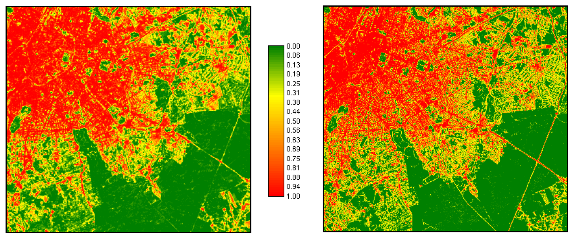
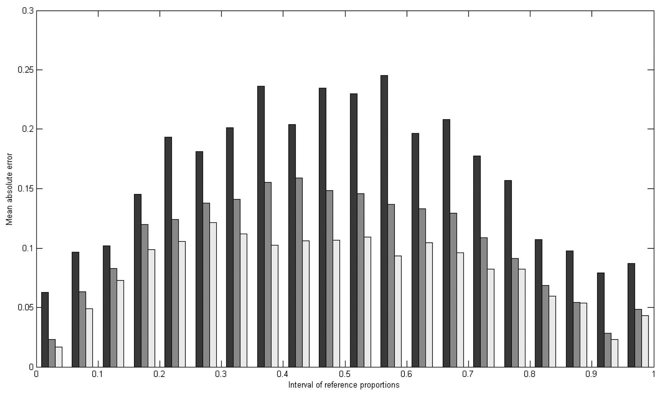
4.1.3. Sub-pixel classification

The six ETM+ multi-spectral bands (1-5, 7), as well as all unique ratios between these bands, were used as variables for building a multiple layer perceptron model for sub-pixel classification. The input variables were mathematically transformed by NeuralWare Predict®. The main purpose of these transformations is to modify the distribution of the input or explanatory variables so that they better match the distribution of the dependent variables [48]. In theory this will optimize the performance of the neural network. The actual input to the neural network was selected by Predict's® genetic algorithm based variable selector. The transformed input channels that were withheld by the variable selection included the following bands and band ratios: B7, B3/B4 (2 transforms), B3/B5, B3/B7, B4/B5. Application of the model to the part of the Landsat ETM+ image that overlaps the Ikonos image resulted in four proportion maps (vegetation, impervious surfaces, water and bare soil). Figure 4 (left) shows the proportion map obtained for impervious surfaces. A visual comparison with the proportion map of impervious surfaces, derived from the Ikonos image (Figure 4, right), shows a good correspondence in the overall pattern of imperviousness, although the sub-pixel classification result is more generalized and includes less structural detail.
Per-class mean errors (MECj) (Table 2) show that impervious surfaces and bare soil are slightly underestimated, while vegetation and water are slightly overestimated. The slight underestimation of impervious surfaces (-1.8 %) may be explained by the presence of shadow in urbanized areas. When examining the estimated proportion of water within the area, it turns out that small portions of many urban pixels have been assigned to water, although no water is present within these pixels. This phenomenon is most clearly observed in dense urban areas and is most likely caused by the presence of shadow, which is spectrally similar to water. As such, the proportion of water identified by the sub-pixel estimator should better be interpreted as water/shade, as it may point to the presence of both components. This may also explain the slight overestimation of water observed in Table 2 (+1.1 %).
The mean absolute error (MAECj) for impervious surfaces and vegetation, which are the two dominant classes in the image, is around 10% (Table 2). Aggregation to cell sizes of 60 m and 90 m reduces this error to 7.5 % and 6.1 % for impervious surfaces, and to 7.2 % and 5.9 % for vegetation. Residual analysis (Figure 5, Figure 6) indicates that the mean absolute error for impervious surfaces and vegetation is the highest (up to 25 % or more) for heterogeneous pixels, where the reference proportion is close to 50 %. Pixels with high or low proportions of impervious surfaces or vegetation (<10 % or >90 %) have much smaller errors (between 5 % and 10 %).
Aggregation to cell sizes of 60 m and 90 m substantially reduces proportional error, especially for pixels with a strongly mixed class composition. As a result of aggregation, the peak value in the graph, indicating which reference proportions have the highest proportional error, seems to shift to lower proportions for impervious surfaces (Figure 5) and to higher proportions for vegetation (Figure 6). For cell sizes of 90 m the average proportional error is the highest for pixels with around 30 % impervious surfaces and around 70 % vegetation.

4.2 Hydrological modelling

The spatial distribution of the WetSpa model parameters for the Woluwe study area were calculated based on the DEM, the soil map, the land-use map, and field measurements of hydraulic properties of the river channel. The period of simulation covers 4 days from May 3, 2005, 1.00 am till May 6, 2005, 9.00 am. This period was selected because of the typical occurrence of a number of spring storms. Since no continuous discharge measurements where available, no formal calibration of the model could be performed. However, some global parameters were adjusted during an initial trial and error calibration procedure, while spatial model parameters were kept constant. The effect of the different land-cover input scenarios on the simulated runoff for the different storms in the period was examined.

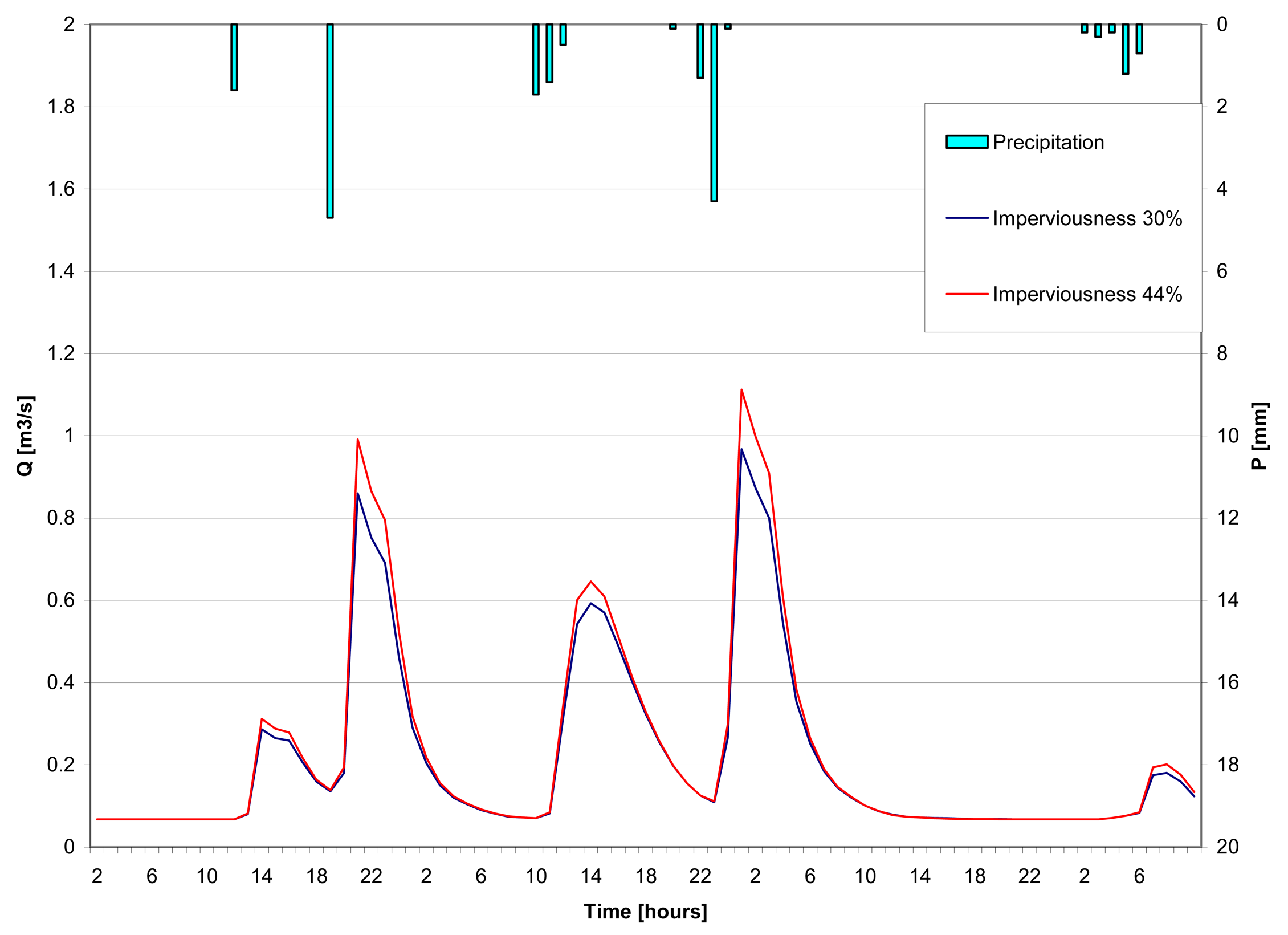
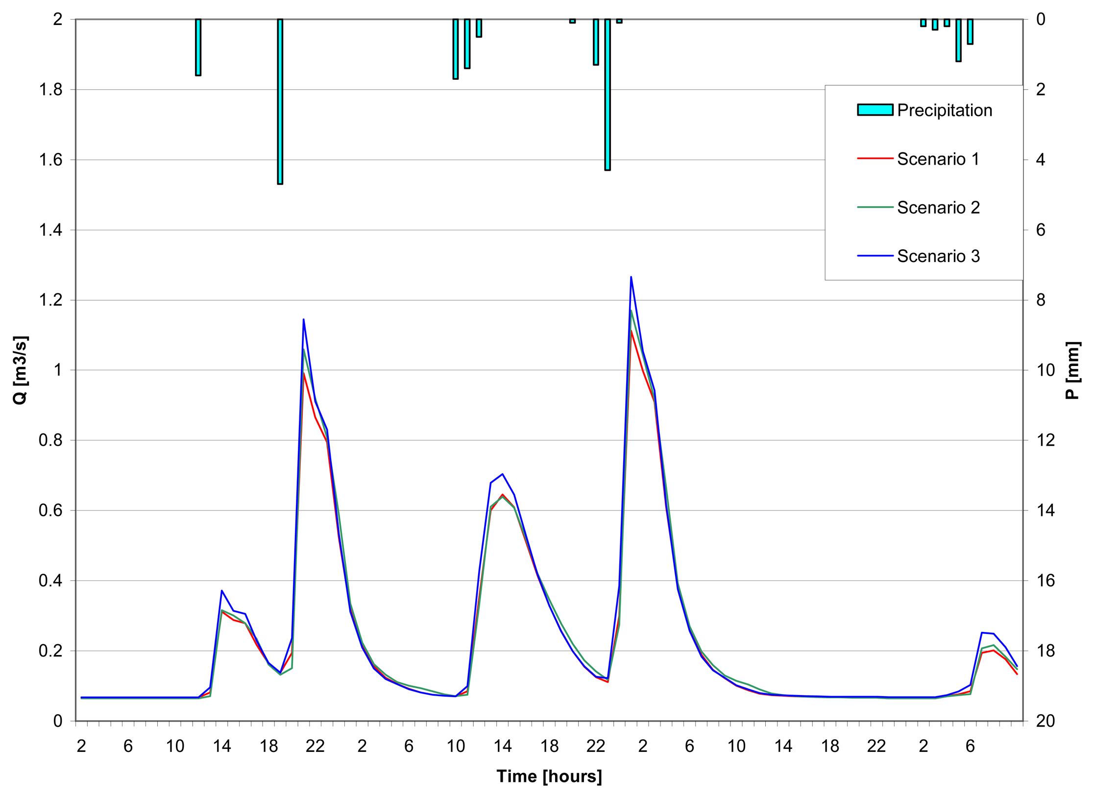
4.2.1 Scenario 1: non-distributed approach

The average levels of imperviousness of the urban area as a whole obtained from the Ikonos land-cover classification and the ETM+ sub-pixel classification prove to be very similar (44 % and 46 % respectively), but substantially differ from the default value for urban areas used in the WetSpa model (30 %). Estimated peak discharges for an average degree of imperviousness of 44 % (Ikonos) are about 10-20 % higher than in the 30 % default scenario (Figure 7).
These results show that remotely sensed imagery may be a valuable data source for improving runoff calculation by providing more realistic estimates of the average degree of imperviousness in urban areas. Both Ikonos high-resolution data and Landsat ETM+ data produce similar estimates of the average degree of imperviousness in the urban part of the catchment, which indicates that medium-resolution data may be a useful alternative for more expensive high-resolution imagery if overall estimates of imperviousness are required. The strong difference in estimated peak discharges for different levels of imperviousness also demonstrates the importance of an accurate estimation of the average level of imperviousness.

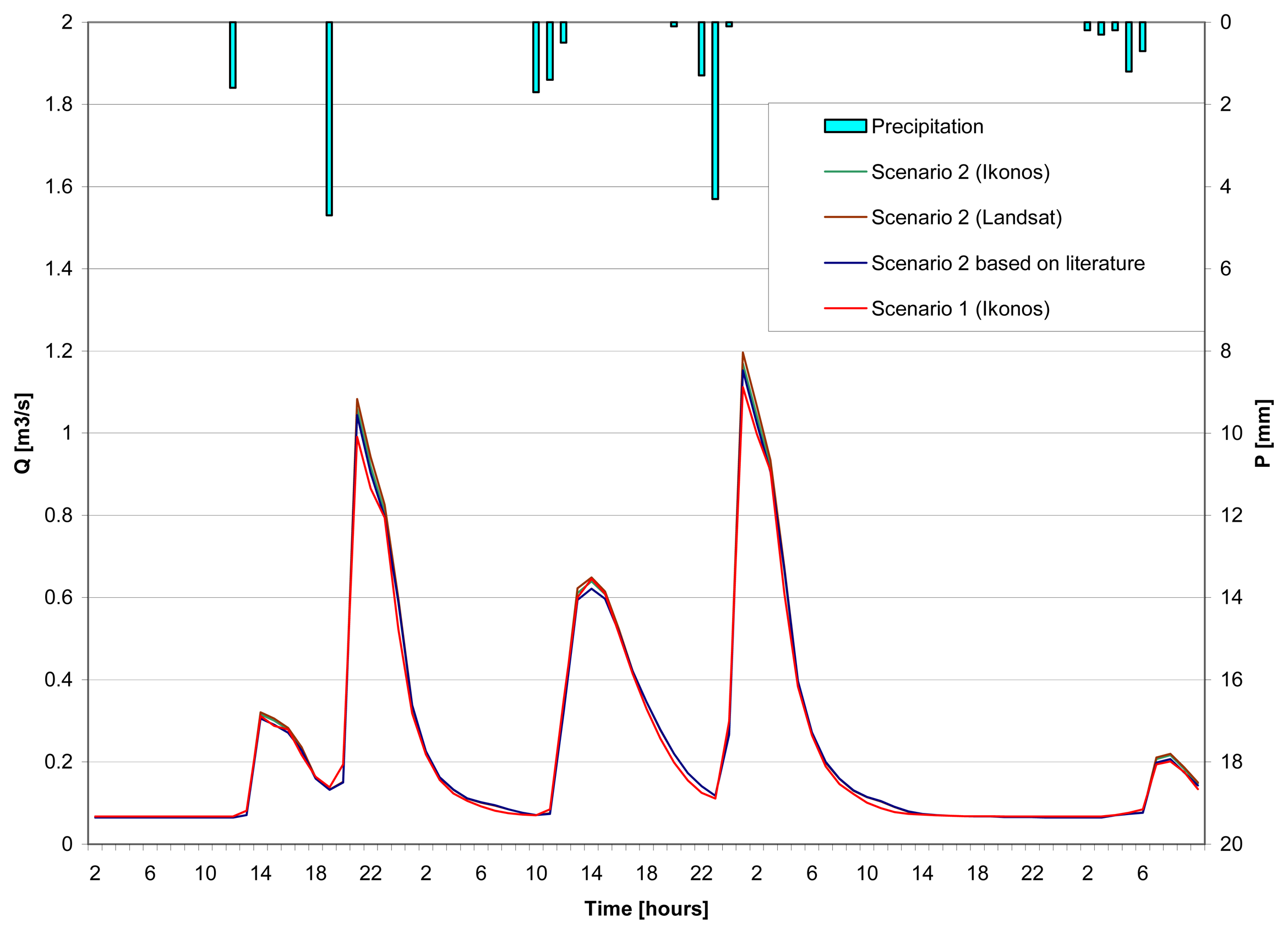
4.2.2 Scenario 2: semi-distributed approach

In this scenario, each of the 6 built-up classes in the land-use map of Flanders was assigned a different level of imperviousness based on the Ikonos-derived and Landsat ETM+-derived proportion estimates. The average degrees of imperviousness for different land-use classes obtained from Ikonos and ETM+ data prove to be similar (Table 3). For some classes, however, remote sensing based levels of imperviousness strongly differ from default values obtained from the literature. This is especially the case for the low-density built-up and city centre classes, where levels of imperviousness are much lower than assumed values. Also for roads and highways remote sensing estimates are lower than the default value. For the high density built-up class, for infrastructure and for industrial area remote sensing estimates are higher than the assumed level of imperviousness. These results again demonstrate the benefit of using remotely sensed data for obtaining more reliable estimates of the average degree of imperviousness for different types of urban land use.
The use of class-specific levels of imperviousness produces maximum peak discharges that are higher than the values obtained by defining one average level of imperviousness for the whole built-up area (between 5 % and 10 % higher for the two most important peaks in rainfall intensity, depending on the method used for estimating class-specific levels of imperviousness) (Figure 8). The map of estimated runoff shows a clear increase in the value of the runoff coefficient in the urbanized area close to the river outlet in the northern part of the catchment, and a decrease in runoff values in areas located further away from the outlet, compared to scenario 1 (Figure 11).
The more pronounced spatial variation in runoff coefficient values, however, seems to have only a minor effect on estimated peak discharges for less intense rainfall events (Figure 8).

4.2.3 Scenario 3: fully-distributed approach

Finally, in scenario 3 each cell in the urban area is assigned its own proportion of impervious surfaces, vegetation, water and bare soil, as obtained from the Ikonos- and Landsat-derived proportion maps. Analysing and comparing the results for the 3 scenarios, the runoff calculated in scenario 3, and based on the Ikonos data, produces the highest peak discharges. The peak discharges are up to 15 % higher than in the non-distributed simulation based on Ikonos data (scenario 1) (Figure 9). Using cell-specific information about the spatial distribution of imperviousness within urban areas seems to have a clear impact on the modelling of peak discharges at the outlet of the catchment and, as such, on flood prediction. Even for less intense rainfall events, the effect of using detailed information on the spatial distribution of impervious surfaces for estimating peak discharges is clear. The spatial variation in runoff is obvious from the map of runoff coefficient values obtained for scenario 3 (Figure 11). High values for the runoff coefficient, in the range of 0.8-1.0, prove to be linked to a closely connected pattern of impervious areas.
The hydrograph simulated in scenario 3, but based on Landsat ETM+ data, has lower peak values than the one based on Ikonos data (Figure 10). In fact, estimated peak discharges based on the use of Landsat ETM+ data for scenario 3 are very similar to the estimates that were obtained with scenario 2. This is most likely due to a smoothing effect in the distribution of impervious surface proportions caused by the sub-pixel classification process, with a direct impact on the spatial variation of runoff coefficient values [49]. The result suggests that sub-pixel estimation of land-cover class proportions based on Landsat ETM+ data is less accurate than high-resolution remote sensing for modelling the spatial distribution of runoff at 30 m cell size. However, if high-resolution data are not available or if resources are limited, the technique may be very useful to account for spatial variation in runoff.

5. Conclusions

In this study a GIS-based distributed hydrological model (WetSpa) was applied to evaluate the effect of different approaches for determining impervious surface cover on estimated peak discharges in the Upper Woluwe catchment (Brussels, Belgium), using high-resolution and medium-resolution remote sensing. The WetSpa model approach allows the use of spatially distributed hydrological parameters of the terrain as inputs to the model, and hence enables the analysis of the effects of land-use parameterization on the hydrologic behaviour of urban basins. Different scenarios focusing on various methods of impervious surface estimation in urban area, assuming a homogeneous distribution of impervious surfaces at the level of the entire urban area, at the level of each urban land-use class, or at the level of the individual pixel, were compared. Also the impact of using land-cover maps obtained by classifying high-resolution imagery (Ikonos) or using estimates of surface imperviousness obtained by sub-pixel classification of medium-resolution data (Landsat ETM+) as an input for runoff modeling was analyzed.
Both high-resolution and medium-resolution imagery are very valuable data sources for improving distributed runoff prediction in urbanized catchments. Multi-spectral classification of high-resolution remotely sensed data (Ikonos) enables accurate mapping of the spatial distribution of sealed surfaces, which proves to be one of the most important factors in the estimation of peak discharges. Also sub-pixel estimation of the fraction of sealed surfaces using medium-resolution imagery (Landsat ETM+) produces reliable estimates of the spatial distribution of sealed surfaces with fraction estimates at the level of individual ETM+ pixels differing less then 10 % on average from estimates derived from high-resolution data.
The highest peak discharges are obtained with the fully-distributed scenario, taking into account the differences in the level of imperviousness for each grid cell in the model. The lowest discharges are obtained with the non-distributed scenario, assuming a homogeneous level of imperviousness for the entire urban area. Including distributed information on surface imperviousness in the simulation of runoff for the Upper Woluwe catchment, making full use of the information obtained from remotely sensed data, obviously leads to higher simulated discharges. The spatial variation in runoff and the role of connectivity between cells with high runoff coefficients seems to be an important factor influencing the discharge volume. Using a fully-distributed hydrological model in combination with spatially distributed information on surface imperviousness derived from remotely sensed data allows one to take into account the important role of connectivity in discharge modeling and, hence, improve flood prediction.
The use of sub-pixel classification models for estimating the amount and the spatial distribution of imperviousness from medium-resolution satellite data is suggested as a cost-effective alternative for the use of more expensive high-resolution data for applications of rainfall-runoff modeling at catchment scale, especially for areas of large extent.

Acknowledgments

The research presented in this paper is funded by the Belgian Science Policy Office in the frame of the STEREO programme - project SR/00/02 (SPIDER). The first author acknowledges the support of the Research in Brussels Programme for a post-doctoral fellowship in 2005.

References

  1. Arnold, J.G.; Srinivasan, S.; Muttiah, R.S.; Williams, J.R. Large area hydrologic modeling and assessment. Part I: Model development. Journal of the American Water Resources Association. 1998, 34, 73–87. [Google Scholar]
  2. Downer, C.W.; Ogden, F.L.; Martin, W.; Harmon, R.S. Theory, development, and applicability of the surface water hydrologic model CASC2D. Hydrol. Process. 2002, 16, 255–275. [Google Scholar]
  3. Borah, D.K.; Xia, R.; Bera, M. DWSM - A dynamic watershed simulation model. In Mathematical Models of Small Watershed Hydrology and Applications; Singh, V.P., Freyert, D.K., Eds.; Water Resources Publications, LLC: Highlands Ranch, Colorado, 2002; pp. 113–166. [Google Scholar]
  4. Fortin, J.P.; Turcotte, R.; Massicotte, S.; Moussa, R.; Fitzback, J.; Villeneuve, J.P. A distributed watershed model compatible with remote sensing and GIS data, I: Description of the model. J. Hydrological Eng. ASCE. 2001, 6, 91–99. [Google Scholar]
  5. Quinn, P.; Beven, K.; Chevallier, P.; Planchon, O. The prediction of hillslope flow paths for distributed hydrological modeling using digital terrain models. Hydrol. Process. 1991, 5, 59–79. [Google Scholar]
  6. Ewen, J.; Parkin, G.; O'Connell, P.E. SHETRAN: distributed river basin flow and transport modeling system. J. Hydrologic Eng. ASCE. 2000, 5, 250–258. [Google Scholar]
  7. Behera, S.; Panda, R.K. Evaluation of management alternatives for an agricultural watershed in a sub-humid subtropical region using a physical process based model. Agriculture, Ecosystems and Environment. 2006, 113, 62–72. [Google Scholar]
  8. Van Der Sande, C.J.; de Jong, S.M.; de Roo, A.P.J. A segmentation and classification approach of IKONOS-2 imagery for land cover mapping to assist flood risk and flood damage assessment. Int. Journal of Applied Earth Observation and Geoinformation. 2003, 4, 217–229. [Google Scholar]
  9. King, C.; Lecomte, V.; Le Bissonnais, Y.; Baghdadi, N.; Souchère, V.; Cerdan, O. Remote-sensing data as an alternative input for the dSTREAMT runoff model. Catena. 2005, 62, 125–135. [Google Scholar]
  10. Brivio, P.A.; Colombo, R.; Maggi, M.; Tomasoni, R. Integration of remote sensing data and GIS for accurate mapping of flooded areas. International Journal of Remote Sensing. 2002, 23, 429–441. [Google Scholar]
  11. Islam, M.; Sado, K. Development priority map for flood countermeasures by remote sensing data with geographic information system. Journal of Hydrologic Engineering. 2002, 7, 346–355. [Google Scholar]
  12. Chormański, J.; Mirosław-Świątek, D.; Okruszko, T. Remote sensing limitation in flood modeling verification in wetlands. In Model Application for Wetlands Hydrology and Hydraulics; Kubrak, J., Okruszko, T., Ignar, S., Eds.; Warsaw Agricultural Press: Warsaw, 2004; pp. 51–72. [Google Scholar]
  13. Baumgartner, M.F.; Apfl, G. Towards an integrated geographic analysis system with remote sensing, GIS and consecutive modeling for snow cover monitoring. International Journal of Remote Sensing. 1994, 15, 1507–1518. [Google Scholar]
  14. Tait, A.B.; Hall, D.K.; Foster, J.L.; Armstring, R.L. Utilizing multiple datasets for snow-cover mapping. Remote Sensing of Environment. 2000, 72, 111–126. [Google Scholar]
  15. Biftu, G.F.; Gan, T.Y. Semi-distributed, physically based, hydrologic modeling of the Paddle River Basin, Alberta, using remotely sensed data. Journal of Hydrology. 2001, 244, 137–156. [Google Scholar]
  16. Kim, G.; Barros, A.P. Space-time characterization of soil moisture from passive microwave remotely sensed imagery and ancillary data. Remote Sensing of Environment. 2002, 81, 393–403. [Google Scholar]
  17. Boegh, E.; Thorsen, M.; Butts, M.B.; Hansen, S.; Christiansen, J.S.; Abrahamsen, P.; Hasager, C.B.; Jensen, N.O.; van der Keura, P.; Refsgaard, J.C.; Schelde, K.; Soegaard, H.; Thomsen, A. Incorporating remote sensing data in physically based distributed agro-hydrological modelling. Journal of Hydrology. 2004, 287, 279–299. [Google Scholar]
  18. Chen, J.M.; Chen, X.; Ju, W.; Geng, X. Distributed hydrologic model for mapping evapotranspiration using remote sensing inputs. Journal of Hydrology. 2005, 305, 15–39. [Google Scholar]
  19. Schueler, T.R. The importance of imperviousness. Watershed Protection Techniques. 1994, 1, 100–110. [Google Scholar]
  20. Arnold, C.A., Jr; Gibbons, C.J. Impervious surface coverage: the emergence of a key urban environmental indicator. Journal of the American Planning Association. 1996, 62, 243–258. [Google Scholar]
  21. Sleavin, W.J.; Civco, D.L.; Prisloe, S.; Gianotti, L. Measuring impervious surfaces for nonpoint source pollution modeling. Proceedings of the ASPRS 2000 Annual Conference, Washington, Dc, 22-26 April; American Society for Photogrammetry and Remote Sensing: Bethesda, MD, 2000. unpaginated CD-ROM. [Google Scholar]
  22. Prisloe, M.; Gianotti, L.; Sleavin, W. Determining impervious surfaces for watershed modeling applications. Proceedings of the 8th National Nonpoint Source Monitoring Workshop, Hartford, Connecticut, 10-14 September; 2000. [Google Scholar]
  23. Cain, A. The usefulness of impervious cover mapping and analysis based on pre-existing classified land use datasets. Proceedings of the 2004 IMAGIN Annual Conference, East Lansing, Michigan; 2004. Available online at: http://www.imagin.org/awards/sp2004/Cain.pdf.
  24. Yang, X.; Liu, Z. Use of satellite-derived landscape imperviousness index to characterize urban spatial growth. Computers, Environment and Urban Systems. 2005, 29, 524–540. [Google Scholar]
  25. Ji, M.; Jensen, J.R. Effectiveness of subpixel analysis in detecting and quantifying urban imperviousness from Landsat Thematic Mapper imagery. Geocarto International. 1999, 14, 33–41. [Google Scholar]
  26. Phinn, S.; Stanford, M.; Scarth, P.; Murray, A.T.; Shyy, T. Monitoring the composition and form of urban environments based on the vegetation–impervious surface–soil (VIS) model by sub-pixel analysis techniques. International Journal of Remote Sensing. 2002, 23, 4131–4153. [Google Scholar]
  27. Wu, C.; Murray, A.T. Estimating impervious surface distribution by spectral mixture analysis. Remote Sensing of Environment. 2003, 84, 493–505. [Google Scholar]
  28. Lu, D.; Weng, Q. Spectral mixture analysis of the urban landscapes in Indianapolis with Landsat ETM+ imagery. Photogrammetric Engineering and Remote Sensing. 2004, 70, 1053–1062. [Google Scholar]
  29. Flanagan, M.; Civco, D.L. Subpixel impervious surface mapping. Proceedings of the ASPRS 2001 Annual Conference, St. Louis, MO, 23-27 April; American Society for Photogrammetry and Remote Sensing: Bethesda, MD, 2001. unpaginated CD-ROM. [Google Scholar]
  30. Wang, Y.; Zhang, X. A SPLIT model for extraction of subpixel impervious surface information. Photogrammetric Engineering and Remote Sensing 2004, 70, 821–828. [Google Scholar]
  31. Huang, C.; Townshend, J.R.G. A stepwise regression tree for nonlinear approximation: applications to estimating subpixel land cover. International Journal of Remote Sensing. 2003, 24, 75–90. [Google Scholar]
  32. Yang, L.; Huang, C.; Homer, C.G.; Wylie, B.K.; Coan, M.J. An approach for mapping large-area impervious surfaces: synergistic use of Landsat-7 ETM+ and high spatial resolution imagery. Canadian Journal of Remote Sensing. 2003, 29, 230–240. [Google Scholar]
  33. Xian, G. Assessing urban growth with sub-pixel impervious surface coverage. In Urban Remote Sensing; Weng, Q., Quattrochi, D.A., Eds.; Taylor & Francis Group: Boca Raton, FL, 2006; p. 179. [Google Scholar]
  34. Hutchinson, M.F. A new procedure for gridding elevation and stream linear data with automatic removal of spurious sinks. Journal of Hydrology. 1989, 106, 211–232. [Google Scholar]
  35. Wang, Z.; Batelaan, O.; De Smedt, F. A distributed model for Water and Energy Transfer between Soil, Plants and Atmosphere. Phys. Chem. Earth. 1996, 21, 189–193. [Google Scholar]
  36. De Smedt, F.; Liu, Y.B.; Gebremeskel, S. Hydrologic modeling on a catchment scale using GIS and remote sensed land use information. In Risk Analysis II; Brebbia, C.A., Ed.; WTI press: Southampton, Boston, 2000; pp. 295–304. [Google Scholar]
  37. Liu, Y.B.; De Smedt, F.; Pfister, L. Flood prediction with the WetSpa model on catchment scale. In Flood Defence ‘2002; Wu, et al., Eds.; Science Press: New York, 2002; pp. 499–507. [Google Scholar]
  38. Linsley, R.K.J.; Kohler, M.A.; Paulhus, J.L.H. Hydrology for Engineers, 3rd Ed. ed; McGraw-Hill: New York, 1982; p. 237. [Google Scholar]
  39. Thornthwaite, C. W.; Mather, J. R. The water balance. In Laboratory of Climatology Publ; No 8, Centerton, NJ, 1955. [Google Scholar]
  40. Wittenberg, H; Sivapalan, M. Watershed groundwater balance estimation using streamflow recession analysis and baseflow separation. Journal of Hydrology. 1999, 219, 20–33. [Google Scholar]
  41. Murphy, D.L. Estimating neighborhood variability with a binary comparison matrix. Photogrammetric Engineering and Remote Sensing. 1985, 51, 667–674. [Google Scholar]
  42. Van de Voorde, T.; De Genst, W.; Canters, F. Improving pixel-based VHR land-cover classifications of urban areas with post-classification techniques. Photogrammetric Engineering and Remote Sensing. 2007, 73, 1017–1027. [Google Scholar]
  43. Taylor, M. Ikonos Planetary Reflectance and Mean Solar Exoatmospheric Irradiance; Space Imaging Inc.: Thornton, Colorado, 2005. URL: http://www.spaceimaging.com/whitepapers_pdfs/Esun1.pdf.
  44. Irish, R.R. Landsat 7 Science Data Users Handbook. Report 430-15-01-003-0; National Aeronautics and Space Administration, Goddard Space Flight Center: Maryland, 2000. URL: http://ltpwww.gsfc.nasa.gov/IAS/handbook/handbook_toc.html.
  45. Liu, Y.B.; De Smedt, F. Flood modeling for complex terrain using GIS and remote sensed information. Water Resources Management. 2005, 19, 605–624. [Google Scholar]
  46. Liu, Y.B. Development and Application of a GIS-based Hydrological Model for Flood Prediction. PhD. Thesis, Vrije Universiteit Brussel, Belgium, Brussel, 2004; p. 315. [Google Scholar]
  47. Van de Voorde, T.; Chormanski, J.; Batelaan, O.; Canters, F. Multi-resolution impervious surface mapping for improved runoff estimation at catchment level. Proceedings of the 1st Workshop of the EARSeL Special Interest Group on Urban Remote Sensing: Urban remote sensing, challenges and solutions, Berlin, Germany, March 2-3; 2006. [Google Scholar]
  48. NeuralWare. NeuralWorks Predict: The Complete Solution for Neural Data Modeling - User Guide; NeuralWare: Carnegie, PA, 2007. [Google Scholar]
  49. Van de Voorde, T.; De Roeck, T.; Canters, F. A comparison of two spectral mixture modelling approaches for impervious surface mapping in urban areas. International Journal of Remote Sensing. accepted.
Figure 1. Location of the Upper Woluwe catchment.
Sensors 08 00910f1
Figure 2. Land use for the Upper Woluwe River catchment (derived from the digital land-use map of Flanders produced by AGIV).
Sensors 08 00910f2
Figure 3. Scatter plot of NDVI of a random sample of ETM+ pixels and the average NDVI of constituent Ikonos pixels before (left) and after temporal filtering (right).
Sensors 08 00910f3
Figure 4. Proportion of impervious surfaces for cells of 30 m resolution obtained by sub-pixel classification of Landsat ETM+ data (left), and by spatial aggregation of the Ikonos derived land-cover map (right) for the area of overlap of both image data sets.
Sensors 08 00910f4
Figure 5. Mean absolute error (MAECj) for impervious surfaces for different intervals of reference proportions and for different levels of aggregation (black: 30 m, grey: 60 m, white: 90 m).
Sensors 08 00910f5
Figure 6. Mean absolute error (MAECj) for vegetation for different intervals of reference proportions and for different levels of aggregation (black: 30 m, grey: 60 m, white: 90 m).
Sensors 08 00910f6
Figure 7. Hydrographs for scenario 1 with 30 % imperviousness (default) and 44 % imperviousness (Ikonos) for the period 3rd of May 2005 1.00 am till 6th of May 2005 9.00 am.
Sensors 08 00910f7
Figure 8. Comparison of hydrographs obtained for scenario 1 and scenario 2 for the period 3rd of May 2005 1.00 am till 6th of May 2005 9.00 am.
Sensors 08 00910f8
Figure 9. Comparison of hydrographs for the 3 scenarios using Ikonos data for the period 3rd of May 2005 1.00 am till 6th of May 2005 9.00 am.
Sensors 08 00910f9
Figure 10. Comparison of hydrographs for scenario 3 using Ikonos data and Landsat data for the period 3rd of May 2005 1.00 am till 6th of May 2005 9.00 am.
Sensors 08 00910f10
Figure 11. Runoff coefficient maps for scenario 1 (upper left), scenario 2 (upper right) and scenario 3 (lower left), based on Ikonos-derived land-cover data, and for scenario 3 (lower right), based on Landsat ETM+-derived land-cover data.
Sensors 08 00910f11
Table 1. Confusion matrix for the high-resolution land-cover map after post-classification improvement of accuracy.
Ground truthSumUser's accuracy
RedBareWaterGrassCropsTreesGrey
ClassificationRed87871.000
Bare1146111490.980
Water1595650.908
Grass12785173370.825
Crops1721721.000
Trees623463540.977
Grey217978000.996
Sum8815460285225354803
Producer's accuracy0.9870.9800.9830.9750.7640.9780.993kappa = 0.947
Table 2. Mean error (MECj) and mean absolute error (MAECj) for the four major land-cover classes for cell sizes of 30 m, 60 m and 90 m.
Mean error (MECj)Mean absolute error (MAECj)

Cell sizeImperviousVegetationBare soilWaterImperviousVegetationBare soilWater
30m-0.0180.015-0.0490.0110.10300.10170.05930.0166
60m-0.0170.014-0.0480.0110.07520.07200.05140.0152
90m-0.0190.015-0.0450.0110.06110.05900.04670.0153
Table 3. Degree of imperviousness for different urban land-use classes: default values and estimates derived from Ikonos data and Landsat data.
Land-use classDefault degree of imperviousnessIkonos-derived valueLandsat-derived value
Low density built-up0.300.120.12
High density built-up0.500.570.61
City centre0.700.450.38
Infrastructure0.500.580.60
Roads/Highways0.500.360.31
Industry0.700.840.86

