A Grain Flow Model to Simulate Grain Yield Sensor Response

Kahramanmaras Sutcu Imam University, College of Agriculture, Department of Agricultural Engineering, 46060 Kahramanmaras, Turkey
Sensors 2008, 8(2), 952-962; https://doi.org/10.3390/s8020952
Submission received: 18 January 2008
/
Accepted: 1 February 2008
/
Published: 9 February 2008
Abstract
:The objective of this study was to develop a flow model for grain combines based on the laboratory and field response of an impact based grain flow sensor. The grain flow model developed in this study is of first order with constant coefficients. A computer code was written to solve the model and to simulate the response of a yield sensor whose response had been determined previously for various types of flow rate inputs both in field and laboratory experiments. The computer program for the simulation can also compensate for the time delay. The simulation results of the theoretical model suited well to the experimental data and showed that the model effectively shows the input-output relationship of grain flow through a grain combine. This model could be used for periodic flow signals acquired from grain yield sensors. It was concluded that the model postulated in this study could be further developed to determine the grain yield entering the combine using the outlet flow rate measured by a yield sensor.
1. Introduction
Amongst other research areas in precision agriculture, developing yield mapping technology is important because yield maps display crop response to the management techniques applied and help identify the causes and effects of yield variability. To generate a yield map, a combine grain flow model is needed so that the amount of grain measured by a yield sensor on a combine could be related to the location of grain in the field.
Amount of grain at a specified location in the field is measured after the crop is processed, usually on or at the exit of the clean grain elevator. Thus, there is a time delay in flow rate measurements, which addresses the time for grain to be transported from the combine head to the yield sensor [1, 2]. To relate the amount of grain measured at the yield sensor to the amount of grain at the combine head, a flow model is needed. This flow model describes the relationship between input and output flow rates and is supposed to shift the flow signal back in accordance with the time delay to determine the exact location of grain in the field [3]. However, it is not possible to reconstruct an exact input signal based on the measured output by using a simple time delay since combine dynamics is more complex than a first order system [3, 4, 5, 6]. Despite the complexities of combine dynamics, first order grain flow models are still in use because of their simplicity and applicability. In essence, the combine dynamics is of higher order. However, better accuracy may not be achieved with the use of a higher flow model as the system becomes more susceptible to errors [4].
One of the earliest studies for yield reconstruction was conducted by Searcy et al. (1989). According to Searcy et al. (1989), the major cause of error in estimating grain yield was the grain flow model. They noted that transfer function determination for each component of the combine was impractical because of the material flow complexity and the difficulty in measuring the flows through each combine component. As a result, the authors assumed a lumped-parameter system to model the grain flow from the combine head to the yield sensor. They concluded that a combine transfer function reconstruction employing a first-order transportation delay could be used to generate grain yield maps. The grain, however, is distributed during the flow of grain inside the combine. The travel time of individual grain kernels from a combine head to grain tank vary substantially as a result of threshing and separating processes [7].
Vansichen and De Baerdemaeker (1991) measured wheat yield continuously on a combine. The inputs of the yield measurement model are yield (YI), combine travel speed (SP), and the actual cutting width (AWI). At each time t, the machine location (x,y)(t) is used to transform the location dependent yield YI(x,y) to a time dependent variable YI(t). The authors stated that the combine acts as a dynamic system with respect to grain flow. FRout, grain transported to the grain tank, is a function of FRin, flow rate at the head. Reitz and Kutzbach (1996) provided an expression that readily employs grain moisture content to calculate yield based on yield YG(t), mass flow rate MG(t), combine ground speed V(t), cutting width W(t), and grain moisture content UG(t) [8].
It has been shown that the scheme for calculating the yield at combine head using the flow rate measured at the yield sensor is in essence the same in the referred studies so far where flow rate, ground speed, and cutting width data are incorporated to derive the yield at the combine head. The studies conducted by Searcy et al. (1989) and Birrell et al. (1996) differ from the others in that they both used paddle wheel flow sensor that does not measure flow rate periodically. The flow signal requires data processing to obtain a periodic signal necessitating further manipulation of the flow data.
Grain flow dynamics may be affected by crop conditions and may vary from one combine model to another. The flow models just reviewed use grain delay time to match the flow data to position data. In doing so, the flow signal was shifted by a constant value of the transportation time delay. These models assume that the grain enters combine and goes through combine components without being disturbed until the flow was measured by the yield sensor. They rely on the assumption that shifting of the flow signal suffices for determining the actual field coordinates of yield. Therefore, the grain mixing and its effects on yield measurements were neglected and modeling grain flow was based on linear, non-mixing grain flow.
Characterizing variation of flow rates inside the combine and how these variations relate to yield variation was studied [9]. It was suggested that it would not be feasible to model all processes within a combine, which mechanistically determine flow rate. They made an assumption that flow rate measured by the yield sensor as a function of time j(t), can be considered as a shift-invariant, linear transform of the flow rate at which crop enters combine head as a function of time, h(t). Then, a convolution function can be established, which relates flow rate j(t), to a characteristic function i(t). This approach is a quick and inexpensive way to characterize the behavior of different combines with different settings, speed and crops. Using the model developed, however, they concluded that the results were not encouraging probably because the sensor noise had been amplified by the deconvolution process. According to Lark et al. (1997), if better than 15 to 20 m is targeted for spatial resolution then remarkable attention must be paid to lessen sensor noise and to enhance the reliability of impulse response function estimation. Whelan and McBratney (1997) investigated grain flow convolution and transport delay to better understand the effects of threshing and transport processes on grain moving through combines. It was found that grain flow indicated by yield monitors was a considerably smoothed representation of the true yield. Both time and frequency domains can be used to examine the continuous time series of grain flow. They further explained that convolution could be difficult to analyze in the time domain and hence could be simplified into a fundamental multiplication operation in the frequency domain. In another study, an analytical approach was chosen in order to maintain the physical insight and the possibility of analyzing the impact of parameter variations on the total dynamic influence. Another reason is the impossibility of measuring the incoming grain flow above the cutterbar of the machine which is necessary for ‘black-box’ identification [10].
The objective of this study was to develop a combine grain flow model that could be further developed to be used as another yield mapping tool for periodic grain flow rate data. Development of such a model consists of two steps. In the first step, the theoretical development of a model needs to be handled, followed by testing the model's applicability in terms of input-output relationship for the grain flow rate. In the second step, the model and the algorithm need to be improved and incorporated with relevant data such as grain moisture content, ground speed, cutting width, slope, GPS data, and clean grain elevator speed, so that it could be better used in a yield mapping tool. Thus the second step comprises the incorporation of actual field data for further development of the model. The scope of this study is limited to the model development, i.e., the first step just described above. The specific objectives of this study were to
- 1)
- derive a combine grain flow model that relates the input and output grain flow rates,
- 2)
- demonstrate through simulation the capability of the model to generate first order signals that are similar to the flow signals obtained previously in field and laboratory experiments using a commercial yield sensor.
2. Materials and Model Development
The field experiments were previously done during corn harvest using a Case IH 2166 and an impact based yield sensor (AgLeader 2000) was used to collect the flow rate data [11]. The yield monitor was mounted at the exit of the clean grain elevator. Laboratory tests were conducted on a test stand described in another study [12] using both the yield monitor and an electronic scale (Weigh-Tronix 1015) for comparison purposes. Corn was used in these tests as well. Flow rate signal that was used as an example in the discussion section of this paper was obtained from the electronic scale. The electronic scale consists of four load cells mounted on the clean grain tank of a test stand that was designed to simulate the clean grain path of a JD 4420 under laboratory conditions. Both the yield sensor and the electronic scale had a measurement error within ±1%. In field experiments, border strips were cut across the rows to introduce step changes in grain flow during actual harvest. This allowed sudden starts and stops in flow rate due to 18 m segment lengths that was emptied from the standing corn rows. In laboratory experiments, grain flow rate was controlled manually by an adjustable opening and was interrupted for 10 seconds to generate step changes in the grain flow. Details on these tests could be found in the referred studies.
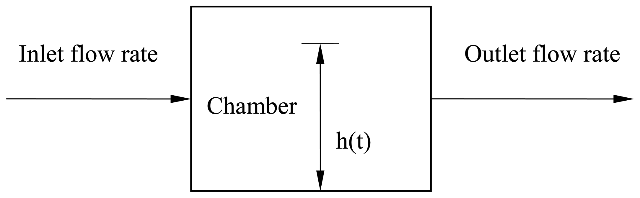
It was mentioned in the previous section that first order models are practical to use while models of higher orders cause errors and noise due to the complexities of combine dynamics. In this study, another first order model was developed that could be used for grain combines. Although this model is to be used just as other first order models referred to in the previous section this postulated model differs in the way the model is derived. According to the postulated model, grain is assumed to flow into a chamber with some form of outlet port. The model is based on the system representation shown in fig. 1.
The following assumptions were made to explain the flow through the closed conduit or a chamber, representing a combine:
- The chamber has a constant cross section with the area of the chamber, A.
- The height of grain in the chamber is h and generally varies with time.
- The outlet port controls the outlet mass flow with the relationship:
Equation 1 expresses that mass flow rate at the outlet is a function of the grain height in the chamber. This very simple model assumes:
According to conservation of mass, the mass flow at the inlet of the chamber would be equal to the mass flow at the outlet port provided that no grain is accumulated in the chamber. Since, according to assumption 2, the height of grain generally varies with time, conservation of mass can be expressed as:
Mass accumulation in the chamber is related to the cross section of the chamber (A), density of the material flowing into the chamber (ρ), and the material height that is time-dependent. Internal rate of mass accumulation thus can be expressed as ρA(dh/dt).
Using the symbols developed so far, equation 4 may be derived, which incorporates the internal rate of mass accumulation:
In equation 4, grain height (h) is not an accessible quantity. The grain height, however, could be expressed in terms of outlet mass flow rate and k given in equation 2. Since the change in mass flow is related to the height of the material in the chamber with the relation mout=kh the rate of change of mass flow is also related to the rate of change of material height in the chamber. This relationship then can be shown as:
Equation 5 can now be used to denote the rate of change of height as follows:
Substituting the latter term into equation 4 results in the following expression:
This first order differential equation can be rearranged yielding equation 8:
Thus the dynamics of mass flow may be expressed in the conventional form for a first order system:
In equation 9, the inaccessible term h in equation 4 is eliminated and the dimensions of k/ρA can be determined. Dimensional analysis results in equation 10:
equation 9 and 10 show that the differential equation is of first order with constant coefficients and hence the quantity ρA/k is the time constant of the system. Using the relationship shown in equation 10, the standard form for the model can be obtained:
Fig. 1 implies that the input flow rate can be determined provided that the output flow rate has been measured and the combine flow model is known. The same holds true for determining the output based on the measured or known input. As far as grain yield measurement and yield mapping are considered, the measured quantity is the output grain flow rate at some point on the clean grain path on a combine, usually at the exit of the clean grain elevator. Instead of estimating the input based on a known output, eq. 12 was used to calculate the output based on a known (step) input. Provided that the output could be successfully determined by using a step input in the model developed, the model and the numerical program could be further developed to determine the input based on actual field data.
A computer program was written to solve the model and various graphs were plotted to see whether grain flow signals that were obtained from grain combines could be simulated. The program can shift flow signal back in time to incorporate the time delay.
3. Results and Discussion
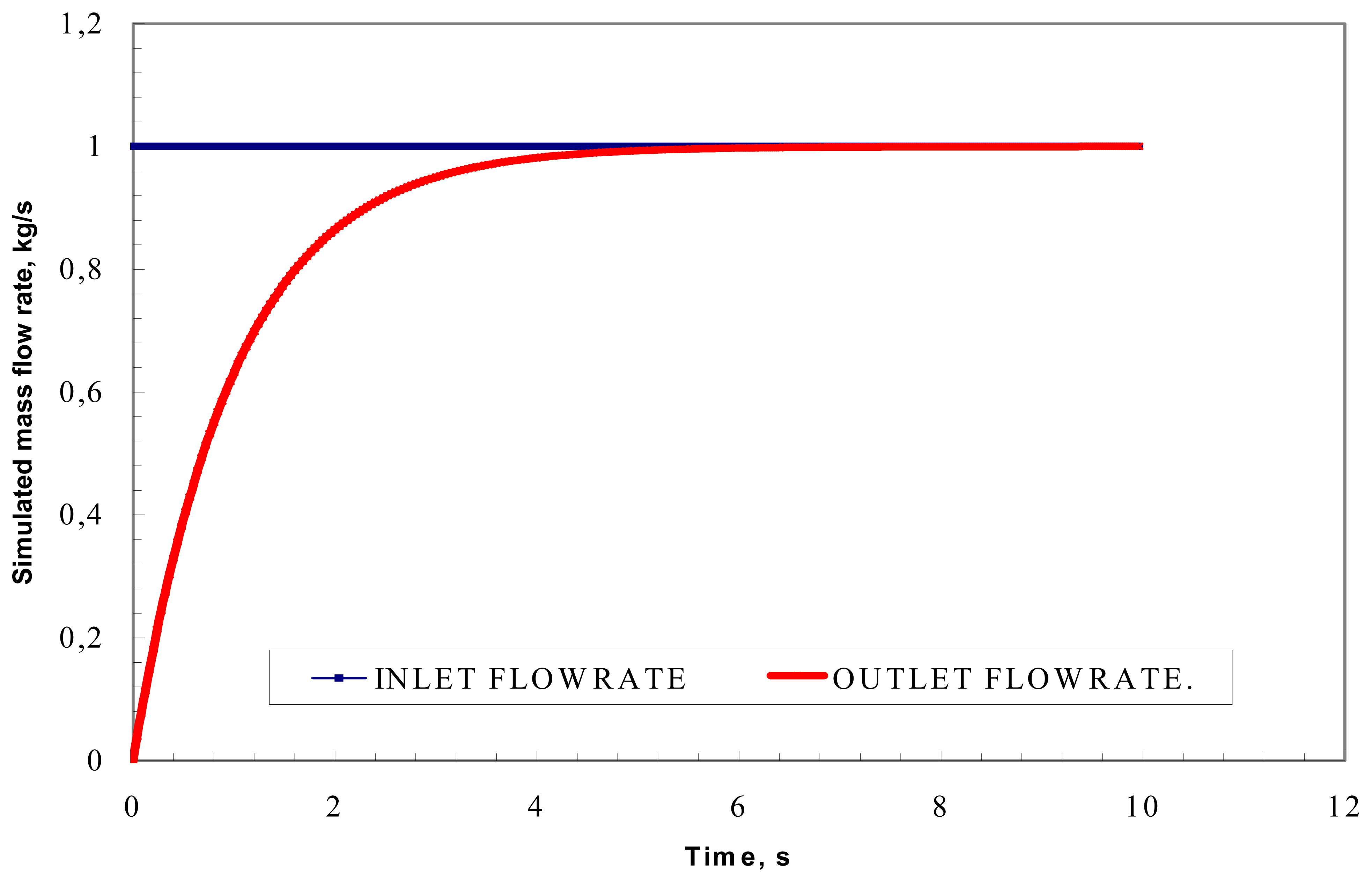
The model expressed in equation 12 was used and the resulting graph found through simulation is given in fig. 2. This is a typical first order response to a unit step input. This figure does not incorporate a time delay, but displays the solution of eq. 12 for duration of 12 seconds with a time constant of 1 s-1. Therefore, fig. 2 simulates the input and output grain flows at the beginning of a harvest strip where grain enters the combine with a flow rate of 1 kg/s and represents a constant flow into the combine. The output signal simulates the grain flow rate measured by the yield sensor at the exit of the clean grain elevator and rises up to 1 kg/s in about 5 seconds. This may not be realistic since the time delay and time constant may differ in field conditions. Nevertheless, the behavior shown in fig. 2 is similar to those flow signals obtained in field and laboratory studies.
Other researchers used filtering techniques when processing grain yield data from a combine harvester. Amongst these are a normal low-pass filter and a filter model based on the characteristics of the machine dynamics, after a low-pass filter [13]. Where the low-pass filtering did not compensate for sudden yield fluctuations because of varying field conditions, machine dynamics filtering partly compensated the fluctuations.
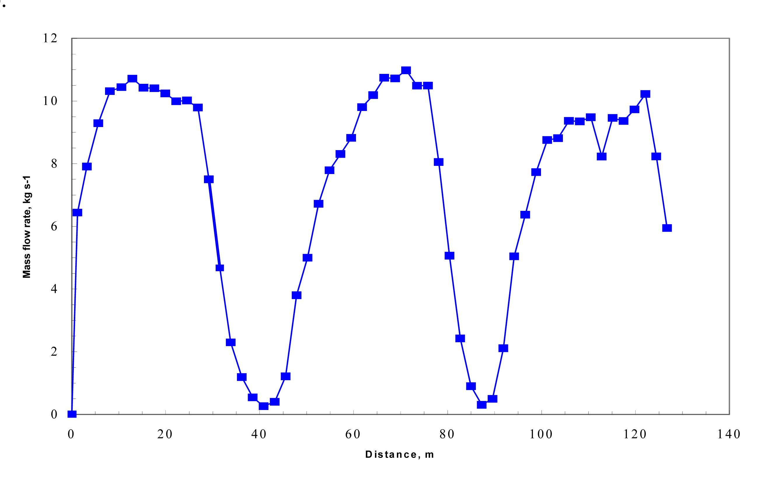
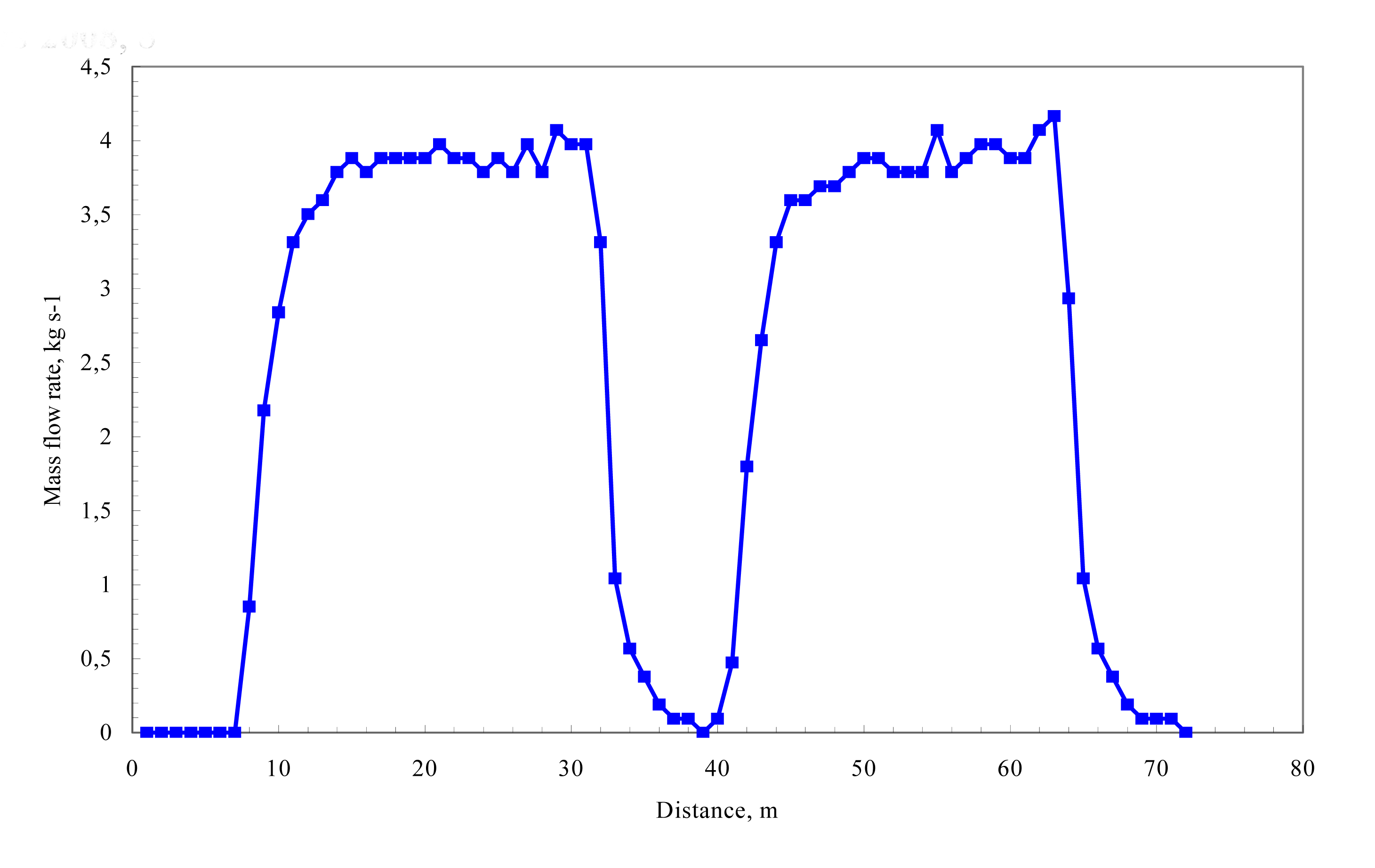
The common feature of the graphs from the laboratory and field experiments is the exponential increases and decreases observed in the beginning and at the end of the tests. This shows that the combine itself behaves like a first order sensor due to the accumulation of grain inside the combine at the beginning of a harvest strip and at sudden yield changes as the harvest continues. Therefore the flow model should be able to simulate field or laboratory responses shown in figures 3 and 4. The simulation result for the unit step response for the theoretical model as shown in fig. 2 was similar in shape to the experimental results in that the output does not rise immediately to follow the input but rounds up.
Thus the shapes of the graphs in figures 2, 3, and 4 suggest that the experimental responses can be modeled as a first order system response as earlier researchers also showed, and can be simulated using a first order flow model such as the one developed in this study. Thus, this simplistic development explains the results that were obtained in both field and laboratory experiments and the model suggests physical meaning.
It is known that the combine transports material through various forms of conduits and this takes time. This means that a disturbance at the input will not be observed at the output until the material has had time to progress through the machine. Fig. 3 depicts that the actual grain flow rate entering the combine could only be measured accurately for approximately 10 s after for this combine harvester. That is, although the actual flow rate was about 10 kg s-1, this magnitude could not be measured by the yield sensor for about 10 seconds. The magnitude of the signal increased exponentially as the grain accumulated and progressed in the combine. Laboratory experiments (fig. 4) reveal the same information in essence, but differ slightly due to the differences between the laboratory test stand and the combine. The laboratory test stand did not have cutting and threshing mechanisms but the clean grain path of a combine. Thus, grain passes through the system and reaches the yield sensor in a shorter time compared to a combine in a field. As a result, the sharpness of rise ups and downs and the time delays had to be different in these two experimental works. Furthermore, the grain flow rate was controlled manually in the laboratory tests. Field experiments did not generate signals as smooth as laboratory tests due to the natural yield variability in the field.
Despite the differences in the flow rate signals in the field and laboratory experiments, there are common characteristics that can be observed. As a result of careful observation of the experimental graphs, one can conclude the following: a constant flow rate input at the beginning of a harvest operation can not be measured by the yield sensor immediately, which necessitates the flow signal to be shifted back in time in accordance with the time delay. Once the yield sensor starts reading flow data points, the magnitude is very small, and hence can not be accurately correlated to the somewhat constant input flow rate. In order words, initial flow rate readings do not give accurate information on the magnitude of the grain flow rate until the grain flow signal reaches its constant value, which is another critical problem that the researchers would like to address in their efforts in generating accurate grain yield maps.
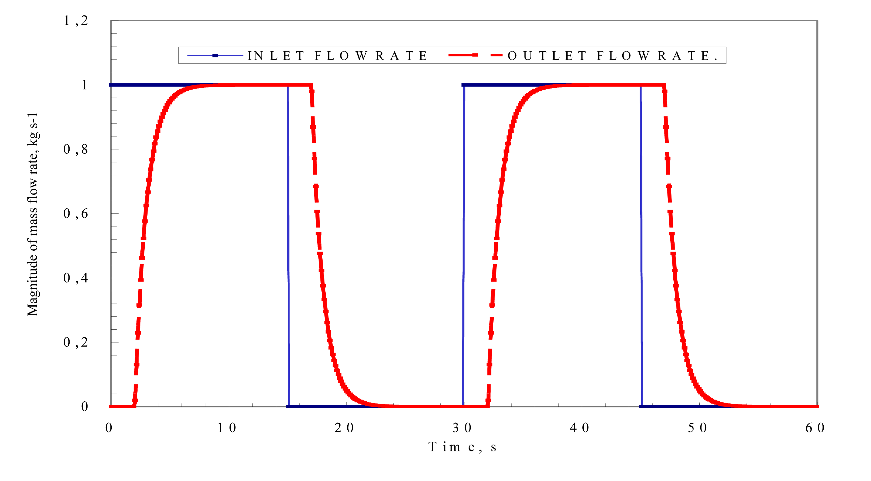
Simulation result shown in fig. 2 did not incorporate a time delay. Based on the discussion above, however, time delay needs to be compensated for so that the resulting graph could resemble the ones in the experimental studies. Therefore the input function was modified in the numerical analysis program to incorporate a time delay. The program can not only compensate for the time delay but the step input changes can be repetitive so that resulting graph could be comparable to the experimental graphs. If the input is made repetitive with 15 s of unit input and 15 s of zero input, i.e. a period of 30 s with a time delay of 2 s for instance, then the simulation appears as in fig 5.
The model seems to explain the experimental results quite satisfactorily. The program is capable of shifting quantities back in time so that the time delay can be compensated based on combine model and grain type being harvested.
This postulated grain flow model may be regarded as simplified, considering the complex dynamics of combines. The result of applying the equation 12, however, to a step input function proved to be useful. The model was able to simulate actual grain flow sensor responses obtained previously in field and laboratory experiments. While this model is also of first order, it differs from the first order flow models previously developed by other researchers in that the combine was represented as a chamber in which the grain height varies with time while inlet and outlet grain flow rates are related via conservation of mass.
The application of the theoretical model that was developed in this study resulted in an acceptable dynamic response for the combine with a flexibility of altering transport delay time of flow signal based on operating conditions.
At this stage of the model development, the time delay as it relates to combine dynamics has been incorporated. The model does not compensate for potential time delays that might result from sensors' responses or monitoring and recording systems. Therefore, future study on this model shall not only focus on including other data such as grain moisture and slope data but also on the effects of monitoring and recording system as well.
The followings could be summarized and concluded as a result of this study:
- A mathematical model was derived for combine grain flow dynamics that relates the input and output grain flow rate that is measured by a grain flow rate sensor.
- The flow model developed is of first order with constant coefficients.
- The simulation results showed that the model effectively shows the input-output relationship of grain flow through a combine.
- The computer program for the simulation can compensate for the time delay.
- The model and the numerical program need to be modified and developed in order to incorporate field data so that the developed model could be used to predict the inlet flow rate based on actual grain flow rate measured by a yield sensor.
Acknowledgments
The help of Prof. Dr. R. J. Smith (Emeritus), Iowa State University, is appreciated in this study.
References and Notes
- Searcy, S.W; Schueller, K.K.; Bae, Y.H.; Borgelt, S.C.; Stout, B.A. Mapping spatially variable yield during combining. Transactions of the ASAE 1989, 2, 826–829. [Google Scholar]
- Vansichen, R.; De Baerdemaeker, J. Continuous wheat yield measurement on a combine. Automated agriculture for the 21 st century. ASAE Publ. 1191 1991, 346–355. [Google Scholar]
- Vansichen, R.; De Baerdemaeker, J. Signal processing and system dynamics for continuous yield measurement on a combine. AgEng'92, Proceedings of an International Conference on Agricultural Engineering, editors: B. Sundell and O. Nored. Upsal, Sweden, Paper No. 92-0601 1992, 340–341. [Google Scholar]
- Birrell, J.S.; Sudduth, K.A.; Borgelt, S.C. Comparison of sensors and techniques for crop yield mapping. Computers and Electronics in Agriculture 1996, 14, 215–233. [Google Scholar]
- Stott, B.L.; Borgelt, S.C.; Sudduth, K.A. Yield determination using an instrumented Class combine. In ASAE Paper No. 93-1507; 1993; St. Joseph, Mich; ASAE USA. [Google Scholar]
- Whelan, B.M.; McBratney, A.B. Sorghum grain flow convolution within a conventional combine harvester. First European Conference on Precision Agriculture, Vol II: Technology, IT and Management, editor: J.V. Stafford. UK 1997, 759–766. [Google Scholar]
- Blackmore, B.S.; Moore, M. Remedial correction of yield map data. Precision Agriculture 1999, 1, 53–66. [Google Scholar]
- Reitz, P.; Kutzbach, H.D. Investigations on a particular yield mapping system for combine harvesters. Computers and Electronics in Agriculture 1996, 14, 137–150. [Google Scholar]
- Lark, R.M.; Stafford, J.V.; Bolam, H.C. Limitations on the spatial resolution of yield mapping for combinable crops. Journal of Agricultural Engineering Research 1997, 66, 183–193. [Google Scholar]
- Maertens, K; De Baerdemaeker, J.; Ramon, H.; De Keyser, R. An analytical grain flow model for a combine harvester, part I: design of the model. Journal of Agricultural Engineering Research 2001, 79, 55–63. [Google Scholar]
- Arslan, S.; Colvin, T.S. An evaluation of the yield monitors and combines to varying yields. Journal of Precision Agriculture 2002, 3, 107–122. [Google Scholar]
- Arslan, S.; Colvin, T.S. Laboratory performance of a yield monitor. Applied Engineering in Agriculture 1999, 3, 189–195. [Google Scholar]
- Reyniers, M.; De Baerdemaeker, J. Comparison of two filtering methods to improve yield data accuracy. Applied Engineering in Agriculture 2005, 3, 909–916. [Google Scholar]
Figure 1.
Schematic representation of grain flow through a combine for the theoretical model.

Figure 2.
Simulated unit step response for the theoretical model.

Figure 3.
Grain yield sensor response to step changes in grain flow on a combine during harvest [11].
Figure 3.
Grain yield sensor response to step changes in grain flow on a combine during harvest [11].

Figure 4.
Grain flow signal as measured by a yield sensor for step changes in grain flow in a laboratory experiment [12].
Figure 4.
Grain flow signal as measured by a yield sensor for step changes in grain flow in a laboratory experiment [12].

Figure 5.
Step response for the theoretical model for repeated inputs.

© 2008 by MDPI Reproduction is permitted for noncommercial purposes.
Share and Cite
MDPI and ACS Style
Arslan, S. A Grain Flow Model to Simulate Grain Yield Sensor Response. Sensors 2008, 8, 952-962. https://doi.org/10.3390/s8020952
AMA Style
Arslan S. A Grain Flow Model to Simulate Grain Yield Sensor Response. Sensors. 2008; 8(2):952-962. https://doi.org/10.3390/s8020952
Chicago/Turabian StyleArslan, Selcuk. 2008. "A Grain Flow Model to Simulate Grain Yield Sensor Response" Sensors 8, no. 2: 952-962. https://doi.org/10.3390/s8020952