Localization Algorithm Based on a Spring Model (LASM) for Large Scale Wireless Sensor Networks

Abstract
:1. Introduction
2. Localization Algorithm based on Spring Model (LASM)
- 1)
- The sensor nodes can be deployed in a two or three-dimensional space. To simplify the explanation, we assume that they are deployed in a two-dimensional space in the rest of the paper.
- 2)
- The wireless sensor network is a dynamic network, which means that the sensor nodes can add in or leave from the network at any time. In addition, the sensor nodes can fail at any moment.
- 3)
- There are at least 3 anchor nodes that know their accurate positions in the wireless sensor network. Other nodes are blind nodes that do not know their positions. The anchor nodes can be realized by GPS or by manual placing in specific positions.
- 4)
- The sensor nodes are able to communicate with neighbor nodes that are in a range of radio range R. They can also distinguish their neighbor nodes by their IDs.
- 5)
- The distance estimates of neighbor nodes can be obtained. It can be realized by RSSI, ToA, TDoA etc as discussed before.
2.1. System model
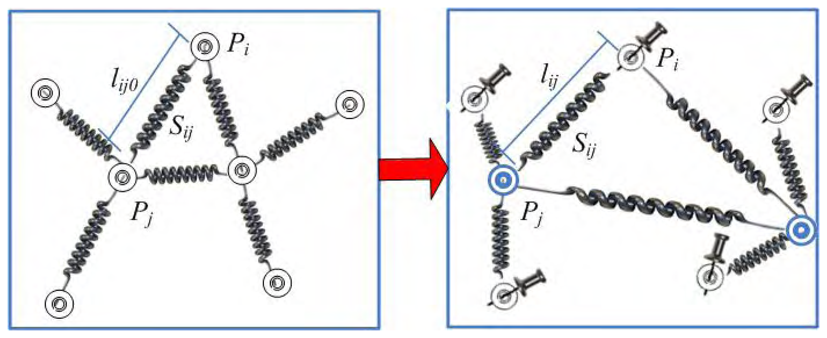
2.1.1 Static and dynamic equations
2.1.2 Localization process
2.2. The basic LASM (LASM(B))
- Step 1:
- InitializationAssign its virtual position at (xi, yi) randomly and its velocity as zero.
- Step 2:
- CommunicationCommunicate with its neighbor particles, obtaining the distances between its neighbor particles and itself (the distances can be calculated by RSSI, TDoA, AoA etc.) and the virtual positions of its neighbors.
- Step 3:
- CalculationCalculate the total force exerted by its neighbors, the acceleration a, and then the next virtual position and velocity using (2)(3)(5). It can be noticed that the next step of position is related with ΔT. The larger the ΔT is, the more rapidly the position changes. Therefore, in the beginning, we set the ΔT larger to let the particle run to the right position more rapidly. After that, we set the ΔT smaller to let the particle adjust its position lightly. Here, we set ΔT be:where c is a constant, l is the number of calculation steps it has run (or the number the particle communicates with its neighbors), and lstep is the upper limited number of steps we set for each particle.
- Step 4:
- IterationRepeat step 2,3 until the total force exerted by neighbors is smaller than a threshold Tforce or l is larger than lstep.
- Step 1:
- each sensor node sends the distances between itself and its neighbors to the sink node. The anchor nodes also send their absolute positions to the sink node.
- Step 2:
- the sink node calculates the positions and velocities for all nodes, using the formula similar with the step3 in the distributed scheme described before.
- Step 3:
- repeat step 2 until the total forces of all particles exerted by neighbors are smaller than a threshold Tforce or l is larger than lstep.
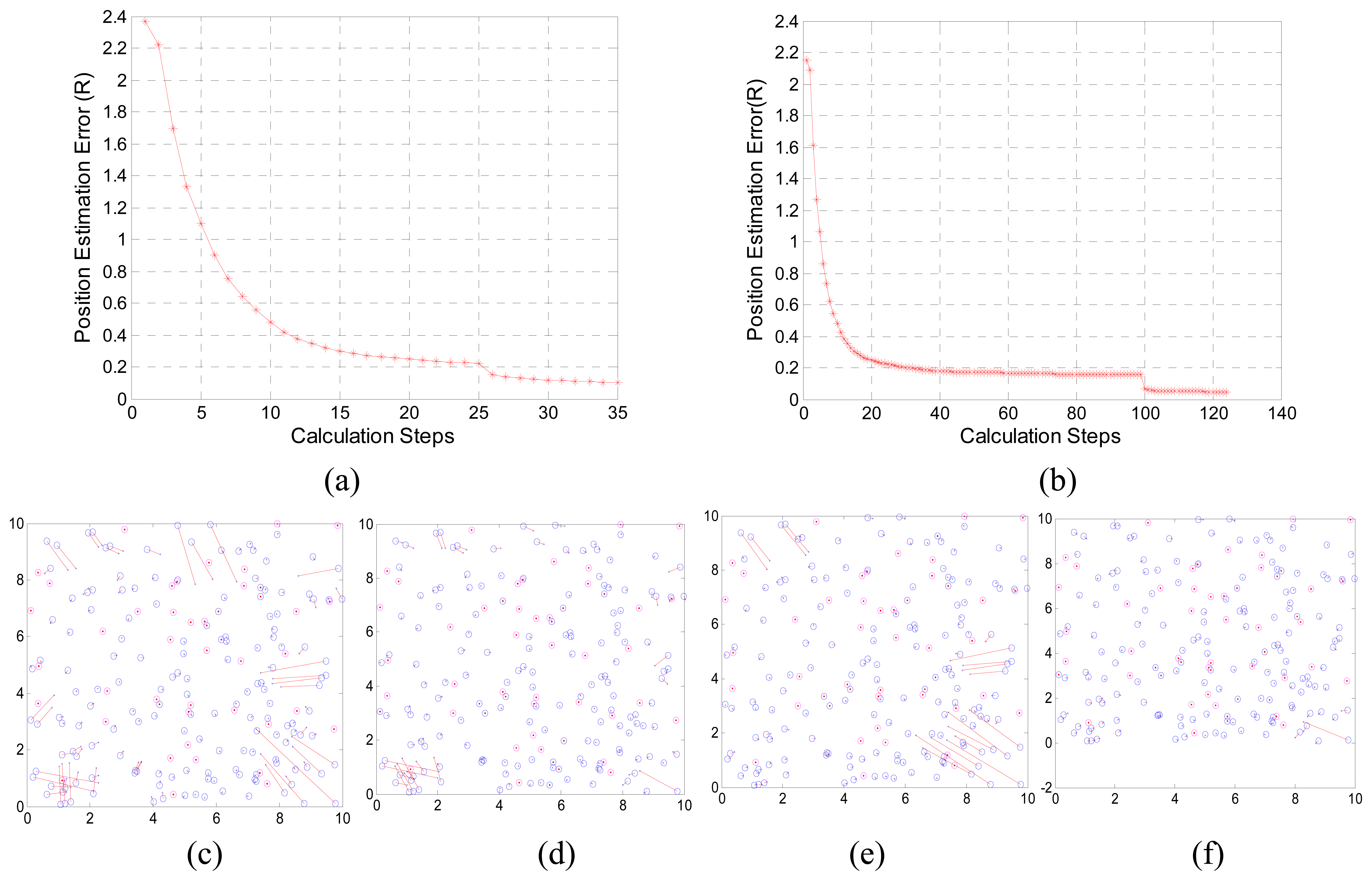
2.2.1 Convergence analysis
2.2.2 Error analysis
2.3. Patches for the basic localization algorithm (LASM(P))
2.3.1 Patch A for particles at needless point
2.3.2 Patch B for bad nodes
- The node cannot be localized;
- The node is localized at needless points.
- Step 1
- for each particle, if it is at needless point, the trust of this particle is set to be 0.5; if it only has one or two neighbor particles, the trust of this particle is set to be 0. The trusts of other particles are set to be 1.
- Step 2
- for each particle, if its trust is not equal to 1, cut off all the springs connected with it. Therefore, it will not be the neighbor particles of others. And then tells its former neighbors to delete itself from the neighbors' neighbor list.
- Step 3
- repeat steps 1&2, until no particles need to change their trust.
2.3.3 Patch C for node variation
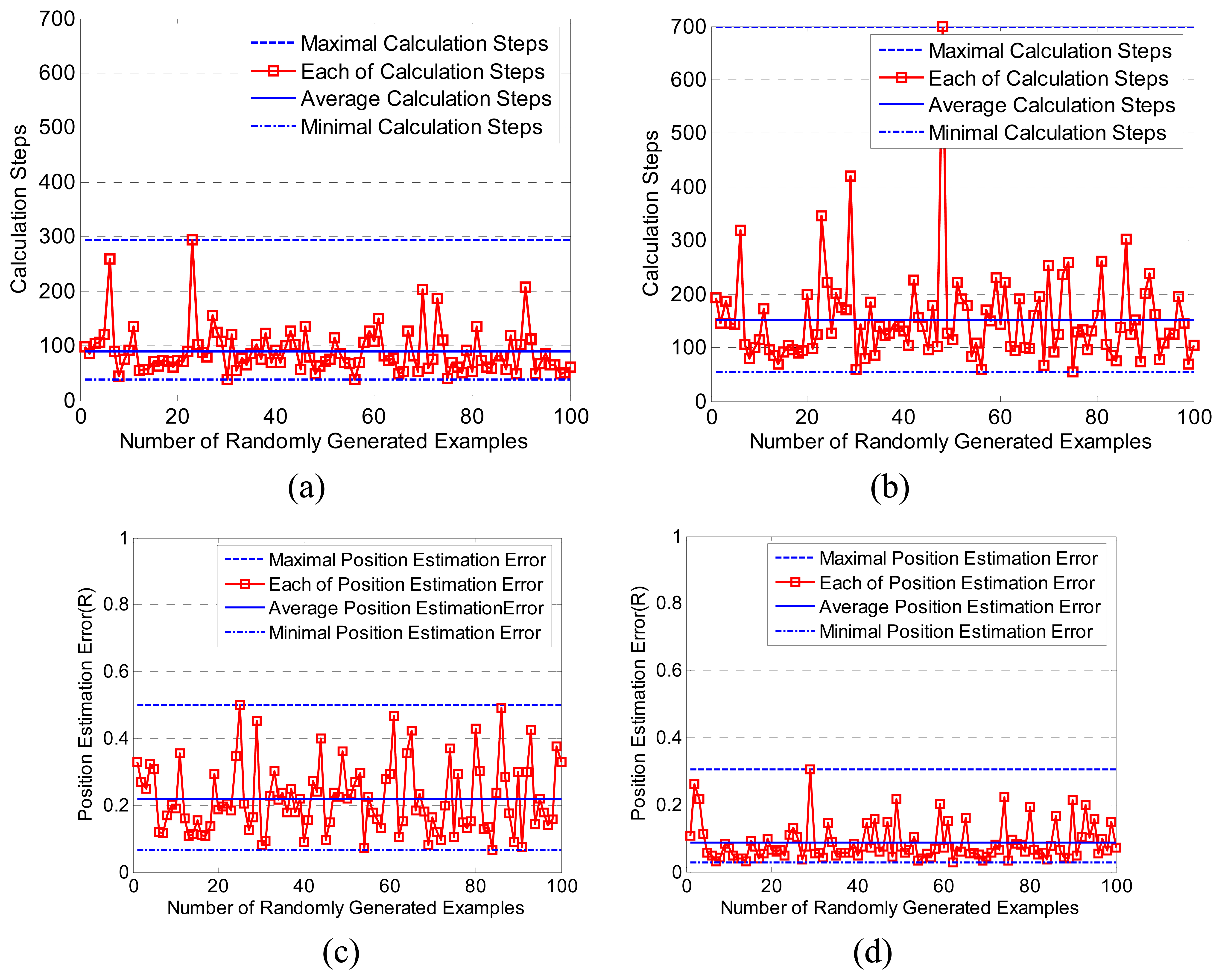
3. Simulation Results
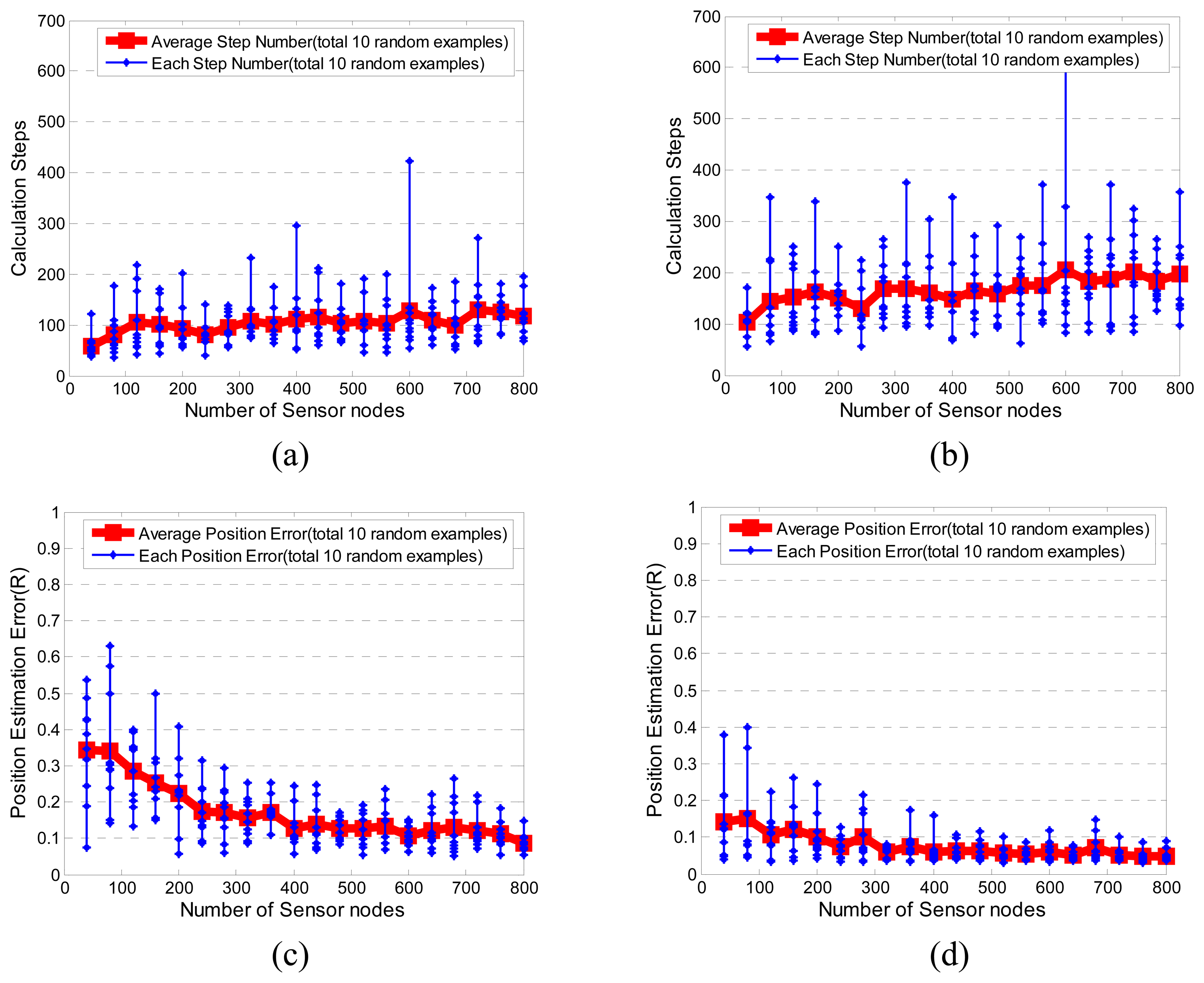
3.1. Performance of LASM(B) and LASM(P)
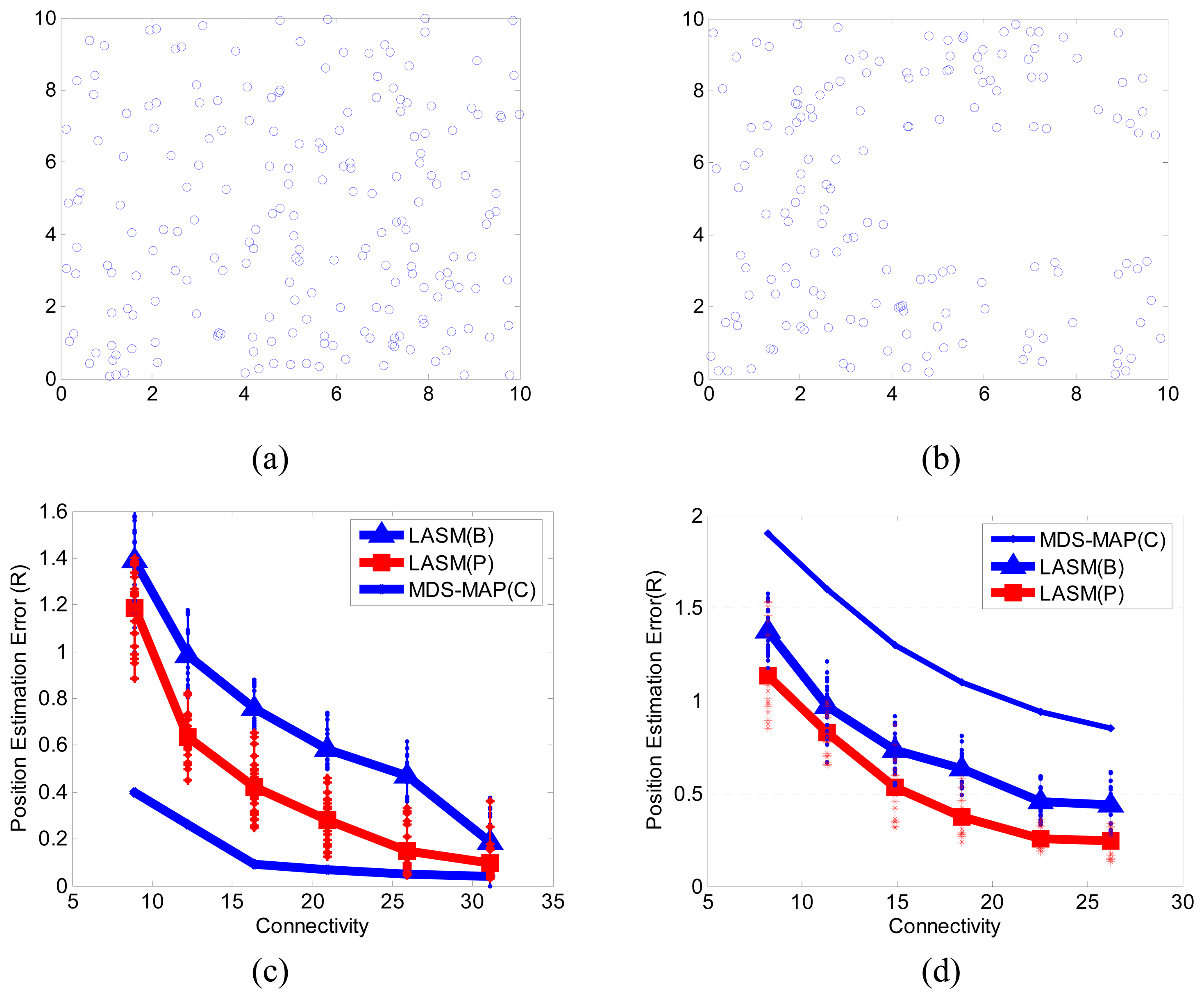
3.2. Comparisons with MDS-MAP
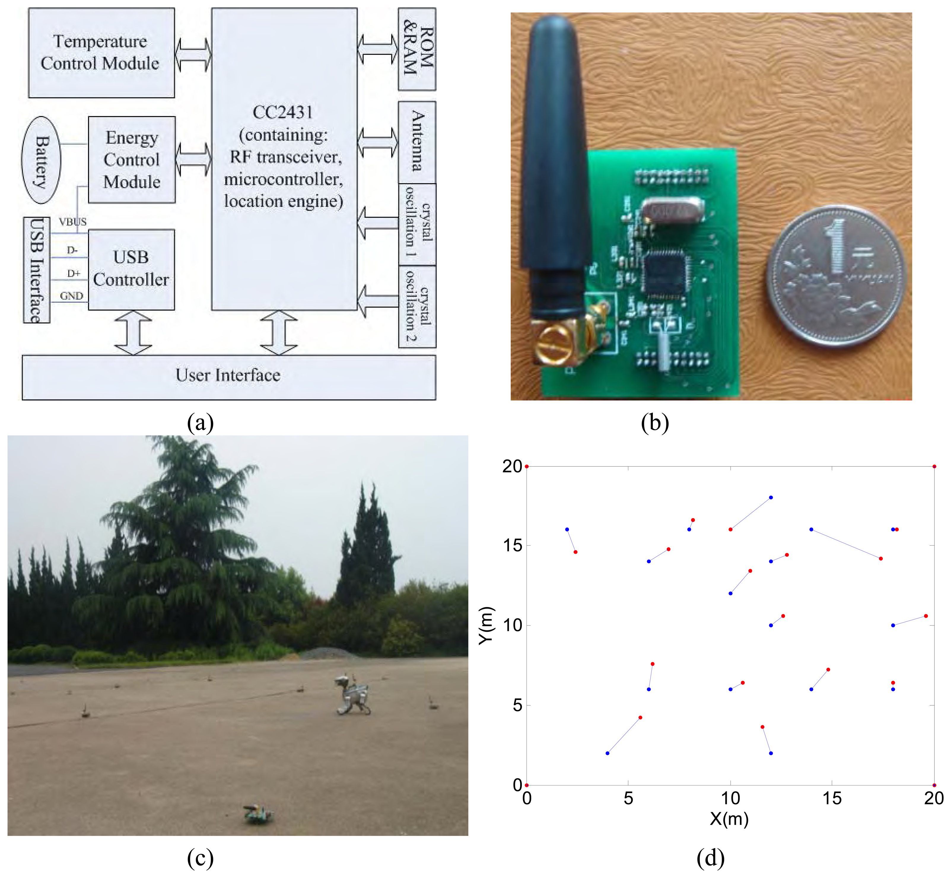
3.3. Initial experiment
4. Conclusions
Acknowledgments
References and Notes
- Deng, Z.; Fang, H.; Dong, Y.; Tao, J. Research on wheel-walking motion control of lunar rover with six cylinder-conical wheels. In IEEE International Conference on Mechatronics and Automation; 2007; Harbin, China; pp. 388–392. [Google Scholar]
- Friedman, L.; Huntress, W. Proposal for an International Lunar Decade. In 36th COSPAR Scientific Assembly 2006; Beijing, China, 2006. [Google Scholar]
- Chen, W.M.; Liang, H.W.; Mei, T. Design and implementation of wireless sensor network for robot navigation. International Journal of Information Acquisition 2007, 4, 77–89. [Google Scholar]
- Khajehnouri, N.; Sayed, A. Distributed MMSE relay strategies for wireless sensor networks. IEEE Transactions on Signal Processing 2007, 55, 3336–3348. [Google Scholar]
- Wang, X.; Bi, D. W.; Ding, L.; Wang, S. Agent collaborative target localization and classification in wireless sensor networks. Sensors 2007, 7, 1359–1386. [Google Scholar]
- Wang, X.; Wang, S.; Ma, J. An improved particle filter for target tracking in sensor system. Sensors 2007, 7, 144–156. [Google Scholar]
- Wang, X.; Wang, S. Collaborative signal processing for target tracking in distributed wireless sensor networks. Journal of Parallel and Distributed Computing 2007, 67, 501–515. [Google Scholar]
- Wang, S.; Shih, K.; Chang, C. Distributed direction-based localization in wireless sensor networks. Computer Communications 2007, 30, 1424–1439. [Google Scholar]
- Yu, Y.; Govindan, R.; Estrin, D. Geographical and energy aware routing: a recursive data dissemination protocol for wireless sensor networks. UCLA Computer Science Department Technical Report 2001. UCLA-CSD-TR-01-0023. [Google Scholar]
- Chen, W.M.; Mei, T.; Li, Y.M.; Liang, H.W.; Liu, Y.M.; Meng, M. Q.-H. An auto-adaptive routing algorithm for wireless sensor networks. IEEE International Conference on Information Acquisition, Jeju City, Korea, July 2007; 2007; pp. 574–578. [Google Scholar]
- Liu, P.X.; Liu, Y. A two-hop energy-efficient mesh protocol for wireless sensor networks. International Journal of Information Acquisition 2004, 1, 237–247. [Google Scholar]
- Wang, X.; Ma, J.; Wang, S.; Bi, D. Cluster-based dynamic energy management for collaborative target tracking in wireless sensor networks. Sensors 2007, 7, 1193–1215. [Google Scholar]
- Liu, C.; Wu, K.; Pei, J. An energy-efficient data collection framework for wireless sensor networks by exploiting spatiotemporal correlation. IEEE Transactions on Parallel and Distributed Systems 2007, 18, 1010–10235. [Google Scholar]
- Liu, P.X.; Ding, N. Data gathering and communication for wireless sensor networks-a centralized approach. International Journal of Information Acquisition 2005, 2, 267–278. [Google Scholar]
- Szu, H. Geometric topology for information acquisition by means of smart sensor web. International Journal of Information Acquisition 2004, 1, 1–22. [Google Scholar]
- He, T.; Huang, C.; Lum, B.; Stankovic, J.; delzaher, T. Range-free localization schemes for large scale sensor networks. In Proc. ACM MobiCom, San Diego, CA, Sep. 2003; 2003; pp. 81–95. [Google Scholar]
- Niculescu, D.; Nath, B. DV based positioning in ad hoc networks. Telecommunication Systems 2003, 22, 267–280. [Google Scholar]
- Savarese, C.; Rabaey, J.; Langendoen, K. Robust positioning algorithms for distributed ad hoc wireless sensor networks. Proceedings of General Track 2002, USENIX Annual Technical Conference 2002. 317–327. [Google Scholar]
- Wong, S.Y.; Lim, J.G.; Rao, S.V.; Seah, W.K.G. Hop-count localization with density and path length awareness in non-uniform wireless sensor networks. Proceedings of IEEE Wireless Communications and Networking Conference, New Orleans, LA, USA, 2005. 13–17 March 2005; 2005. [Google Scholar]
- Sit, T.; Liu, Z.; Jr, M.H.; Seah, W. Multi-robot mobility enhanced hop-count based localization in ad hoc networks. Robotics and Autonomous Systems 2007, 55, 244–252. [Google Scholar]
- Lai, X.Z. New distributed positioning algorithm based on centroid of circular belt for wireless sensor networks. International Journal of Automation and Computing 2007, 4, 315–324. [Google Scholar]
- Vivekanandan, V.; Wong, V. Concentric anchor beacon localization algorithm for wireless sensor networks. IEEE Transactions on Vehicular Technology 2007, 56, 2733–2744. [Google Scholar]
- Savvides, A.; Han, C.C.; Srivastava, M. Dynamic fine-grained localization in ad hoc networks of sensors. Proc. ACM/IEEE Int'l Conf. Mobile Computing and Networking (MOBICON) 2001. [Google Scholar]
- Shang, Y.; Ruml, W.; Zhang, Y.; Fromherz, M. Localization from connectivity in sensor networks. IEEE Transactions on Parallel and Distributed Systems 2004, 15, 961–974. [Google Scholar]
- Shang, Y.; Ruml, W.; Zhang, K.; Fromherz, M. Localization from mere connectivity. ACM MobiHoc, Annapolis, MD, June 2003; 2003; pp. 201–212. [Google Scholar]
- Shang, Y.; Ruml, W. Improved MDS-based localization. INFOCOM 2004, 2640–2651. [Google Scholar]
- Heiken, G.; Vaniman, D.; French, B. Lunar Sourcebook: A User's Guide to the Moon; Cambridge Univ Press, 1991. [Google Scholar]
- Miao, S.F.; Liang, H.W.; Meng, M. Q.-H.; Chen, W.M.; Li, S. Design of wireless sensor networks nodes under lunar environment. Transducer and Microsystem Technologies 2007, 26, 117–120. [Google Scholar]

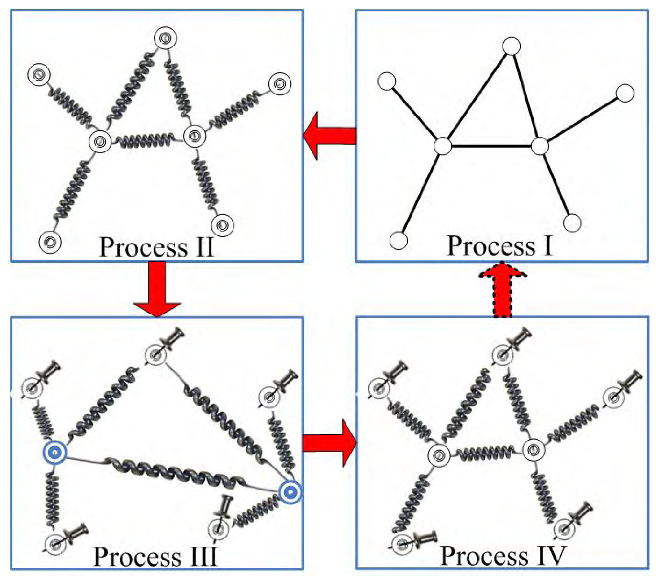
- wireless sensor network
- Spring model.
- Drawing blind particles in random positions
- Blind particles go back to their stable positions
- wireless sensor network
- Spring model.
- Drawing blind particles in random positions
- Blind particles go back to their stable positions


| Distributed LASM(B) | Distributed LASM(P) | MDS-MAP(P) | |
|---|---|---|---|
| Communication Cost | O(1)*n | O(1)*n | O(n log n) |
| Centralized LASM(B) | Centralized LASM(P) | MDS-MAP(C) | |
| Computational Complexity | O(1)*n | O(1)*n | O(n3) |
© 2008 by MDPI Reproduction is permitted for noncommercial purposes.
Share and Cite
Chen, W.; Mei, T.; Meng, M.Q.-H.; Liang, H.; Liu, Y.; Li, Y.; Li, S. Localization Algorithm Based on a Spring Model (LASM) for Large Scale Wireless Sensor Networks. Sensors 2008, 8, 1797-1818. https://doi.org/10.3390/s8031797
Chen W, Mei T, Meng MQ-H, Liang H, Liu Y, Li Y, Li S. Localization Algorithm Based on a Spring Model (LASM) for Large Scale Wireless Sensor Networks. Sensors. 2008; 8(3):1797-1818. https://doi.org/10.3390/s8031797
Chicago/Turabian StyleChen, Wanming, Tao Mei, Max Q.-H. Meng, Huawei Liang, Yumei Liu, Yangming Li, and Shuai Li. 2008. "Localization Algorithm Based on a Spring Model (LASM) for Large Scale Wireless Sensor Networks" Sensors 8, no. 3: 1797-1818. https://doi.org/10.3390/s8031797