Energy-efficient Organization of Wireless Sensor Networks with Adaptive Forecasting

State Key Laboratory of Precision Measurement Technology and Instrument, Department of Precision Instruments, Tsinghua University, Beijing 100084, P. R. China
*
Author to whom correspondence should be addressed.
Sensors 2008, 8(4), 2604-2616; https://doi.org/10.3390/s8042604
Submission received: 2 April 2008
/
Accepted: 10 April 2008
/
Published: 11 April 2008
Abstract
:Due to the wide potential applications of wireless sensor networks, this topic has attracted great attention. The strict energy constraints of sensor nodes result in great challenges for energy efficiency. This paper proposes an energy-efficient organization method. The organization of wireless sensor networks is formulated for target tracking. Target localization is achieved by collaborative sensing with multi-sensor fusion. The historical localization results are utilized for adaptive target trajectory forecasting. Combining autoregressive moving average (ARMA) model and radial basis function networks (RBFNs), robust target position forecasting is performed. Moreover, an energy-efficient organization method is presented to enhance the energy efficiency of wireless sensor networks. The sensor nodes implement sensing tasks are awakened in a distributed manner. When the sensor nodes transfer their observations to achieve data fusion, the routing scheme is obtained by ant colony optimization. Thus, both the operation and communication energy consumption can be minimized. Experimental results verify that the combination of ARMA model and RBFN can estimate the target position efficiently and energy saving is achieved by the proposed organization method in wireless sensor networks.
1. Introduction
Wireless sensor networks (WSNs) have become a growing research field. In WSN, a large number of intelligent sensor nodes with sensing, processing and communication capabilities accomplish complicated sensing tasks. Due to the limited battery capacity, the energy efficiency of a WSN is an important issue. Sleeping and awakening of sensor nodes are supported in power-aware hardware design [1]. As a typical WSN application, target tracking should be addressed as an energy efficiency problem. Prior target position estimation can be used to organize the awakening and routing of WSN, so that the energy efficiency can be improved. Traditional target tracking is usually performed by a Kalman filter (KF) [2] or a particle filter (PF) [3]. These algorithms are computationally-intensive for sensor nodes. Here, adaptive estimation can be provided by autoregressive moving average (ARMA) models. However, the high uncertainty around maneuvers, which brings estimation error into the forecasting process, must be handled. Based on the forecasted results, energy-efficient organization of sensor nodes can be performed to optimize the energy consumption of a WSN.
This paper proposes an energy-efficient organization method for WSNs. Equipped with multi-sensors, sensor nodes can produce range and bearing measurements. As the target is often detected by a number of sensor nodes, a Fisher information matrix (FIM) [4] is adopted to evaluate the target localization error. With the known target trajectory, adaptive target position forecasting is implemented by a novel algorithm. It is a combination of ARMA model [5] and RBFN [6], which is called ARMA-RBF. The target position estimation of the next sensing instant is available. The energy-efficient organization approach includes sensor node awakening and dynamic routing. A distributed awakening approach is presented to save and scale the operation energy consumption. Ant colony optimization (ACO) [7] is introduced to optimize the routing scheme, where transmission energy consumption is concerned. Experiments analyze the energy efficiency of proposed energy-efficient organization method and present the energy saving.
The rest of this paper is organized as follows. Section II gives the preliminaries of the energy-efficient organization for target tracking. In Section III, we present the principle of collaborative sensing and adaptive estimation. Section IV describes the approach of energy-efficient organization, including sensor node awakening and dynamic routing scheme. Experimental results are provided by Section V. Finally, Section VI presents the conclusions of the paper.
2. Preliminaries
The two-dimension sensing field is filled with randomly deployed sensor nodes. Their positions are provided by a global positioning system (GPS). A sink node is located in the centre of the sensing field. Sensor nodes sense collaboratively within a specified sensing period [8]. As the historical target positions become available, the sink node can forecast the target position of the next sensing period.
2.1 Multi-Sensor Model
It is assumed that each sensor node equips two kinds of sensors, one pyroelectric infra-red (PIR) sensor and one omni-microphone sensor. Sensor nodes obtain the bearing observations with the PIR sensors, while the range observations are produced by the omni-microphone sensors. For each sensor node, it is assumed that the two sensors have the same sensing range Rs. The coordinates of the sensor node and target are denoted by
and (xtarget, ytarget) respectively. Then the true bearing angle is calculated as:
and the true range value is calculated as:
Both sensors have zero-mean and Gaussian error distribution. The standard deviation of bearing and range observations is σβ and σr respectively. The observations produced by the sensor node i are:
where wb and wr are the corresponding Gaussian white noise.
2.2 Energy Model
For the scalability of energy consumption in WSN, all the components of the sensor node are supposed to be controlled by an operation system, such as micro Operating System (μOS) [1]. Thereby, shutting down or turning on any component is enabled by device drivers in the specified WSN application.
During sensor node operation, four main parts of energy consumption source are considered: processing, sensing, reception and transmission. The processing energy is spent by the processor with memory. It is assumed that when the processor is active it has constant power consumption. The embedded sensors and A/D converter are adopted as there is any sensing task, and the corresponding power consumption is a constant. For wireless communication, the reception and transmission energy is derived from the RF circuits.
When the reception portion is turned on, the sensor node keeps listening to the wireless channel or receiving data. For the transmission portion of RF circuits, the transmission amplifier has to achieve an acceptable magnification. Therefore, when sensor nodes i transmits data to sensor node j, the power consumed by transmission portion is [9]:
where rd denotes the data rate, α1 denotes the electronics energy expended in transmitting one bit of data, α2 > 0 is a constant related to transmission amplifier energy consumption, di,j is the Euclidean distance between the two sensor nodes.
3. Collaborative Sensing and Adaptive Estimation
Due to the redundancy of sensor node deployment in WSNs, the target can be detected by a group of sensor nodes simultaneously. Observations of sensor nodes are merged for higher detection accuracy. Moreover, the sink node constructs the forecasting model with the historical target trajectory.
3.1 Target Localization with Multi-sensor Fusion
It is assumed that the coordinates of the target are (xtarget , ytarget) at one sensing instant of the WSN. Meanwhile, the target can be detected by Ns sensor nodes. Sensor nodes can produce the bearing observations βi and range observations ri , where i =1,2, ⋯ , Ns. For sensor node i, the matrix representation of the observation equation can be derived from (3) and (4):
where X = [xtarget , ytarget]T is the true target position, Γ i = [βi ,ri]T is the observation vector, Hi is the observation matrix, Wi is the observation error vector, N means the normal distribution function, and
.
With the observation of the sensor node i , the likelihood function of the true target position X is calculated as:
A suitable measure for the information contained in the observations can be derived from the Fisher information matrix (FIM) [4]. The FIM for the observations of sensor node i is calculated as:
where E represents the expected value.
According to (7), we have:
where
,
and
is the Euclidean distance between the true target position and sensor node i as presented in (2).
is the estimation error covariance matrix, which defines the Cramer-Rao lower bound (CRLB). To localize the target with higher accuracy, we should extract the information from the all the observations {Γi |i = 1,2, ⋯ , Ns}. The FIM for all the observations is calculated as:
According to the estimation error covariance matrix J−1, the root mean square error (RMSE) Le is taken as the target location error, which is calculated as:
where trace is a function computing the sum of matrix diagonal elements.
In this way, the target can be localized by maximum likelihood estimation after gathering the observations from the sensor nodes. The location accuracy is reflected by Le.
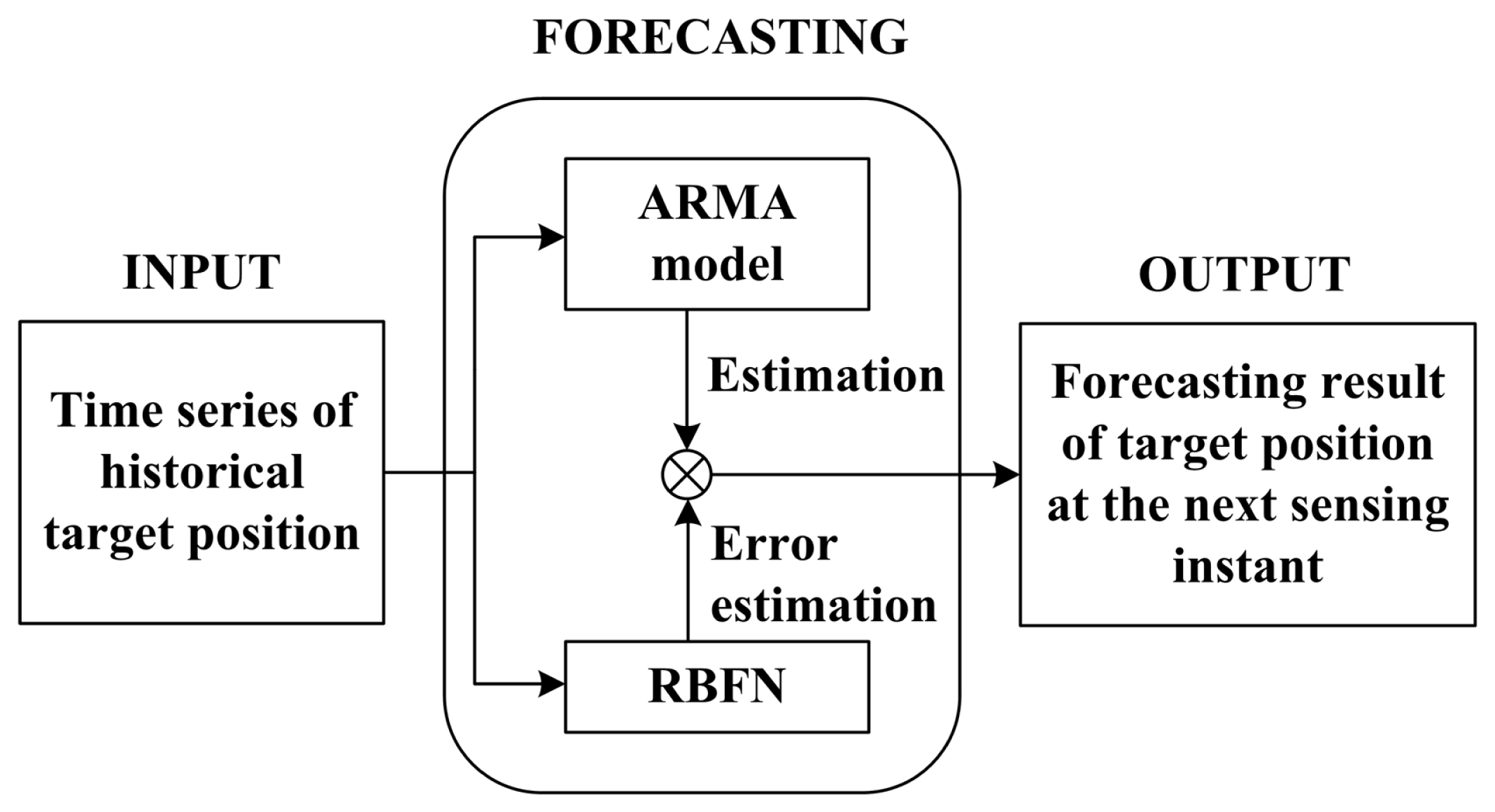
3.2 Adaptive Target Position Forecasting
As a record of the target trajectory, a time series of historical target positions is transferred among the sensor nodes with sensing tasks. When the current target position is obtained, the historical target is also available in the active sensor nodes so that target forecasting can be performed. In the two-dimension field, the target position is presented by Descartes coordinates. One direction of the target trajectory {yk | k =1,2, ⋯, Nt} is considered for this discussion. The problem is to estimate the target position yNt+1 in the next sensing period. The same forecasting approach can be implemented in the other direction.
The ARMA model is adopted here due to its outstanding performance in model fitting and forecasting and its modest computational burden. The ARMA model contains two terms, the autoregressive (AR) term and the moving average (MA) term [5]. In the AR process, the current value of the time series yk is expressed linearly in terms of its previous values {yk−1, yk−2,⋯ yk−p} and a random noise a . This model is defined as a AR process of order p , AR( p) . It can be presented as:
where {ϕi |i =1,2,⋯, p } are the AR coefficients. In the MA process, the current value of the time series yk is expressed linearly in terms of current and previous values of a white noise series {ak ,ak−1,⋯, ak-q}. This noise series is constructed from the prediction errors. This model is defined as a MA process of order q , MA(q). It can be presented as:
In the autoregressive moving average process, the current value of the time series yk is expressed linearly in terms of its values at previous periods {yk−1, yk−2,⋯,yk−p} and in terms of current and previous values of a white noise {ak, ak−1, ⋯, ak−q}.
To determine the order of ARMA model, the patterns of autocorrelation function (ACF) and partial autocorrelation function (PACF) are analyzed. After experimental analysis, it is found that the time series {yk |k =1,2, ⋯, Nt} can be modeled by AR(p) . The method of least square estimation is adopted to determine the coefficients of AR(p) [10].
With the constructed AR(p) model, forecasting can be performed on sensor nodes. In general, the estimation equation of yNt+1 is:
Compared to (12), the noise term ap+1 is not taken into account. To enhance the accuracy and robustness of forecasting, the estimation ȃp+1 of ap+1 is obtained by RBFN.
RBFN is a three-layer feed-forward neural network which is embedded with several radial-basis functions. Such a network is characterized by an input layer, a single layer of nonlinear processing neurons, and an output layer. The output of the RBFN is calculated according to [11]:
where zin is an input vector, χj is a basis function, ‖·‖2 denotes the Euclidean norm, ωj are the weights in the output layer, M is the number of neurons in the hidden layer, and cj are the centers of RBF in the input vector space. The functional form of cj is assumed to have been given, which is always assumed as Gaussian function:
where σ is a constant.
Input vector [yi yi+1 ⋯ yi+p−1] and output ai+p are taken as the training samples, where 1 ≤ i ≤ Nt − p. Then the estimation y̑Nt+1 is calculated as:
In ARMA-RBF algorithm, the RBFN is dynamically trained with the new target position in each sensing period. With the output of RBFN, the forecasting error of ARMA model can be compensated.
4. Energy-Efficient Organization Method
With the forecasted target position, WSN performs distributed awakening to enhance the scalability of the energy consumption. Moreover, the routing scheme of data reporting is optimized by ACO for energy efficiency.
4.1 Distributed Sensor Node Awakening
Sensor node awakening is considered with the forecasted target position. To prolong the lifetime of WSN, we exploit a sensor node awakening approach. Operation modes of sensor node are defined as follows:
- 1)
- Sleep: It has the lowest power consumption as all the components are inactive. Only the timer-driven awakening is supported, that is, the processor component can be awakened by its own timer. The power consumption is defined as 5mW.
- 2)
- Idle: Only the processor component is active in this mode. All the other components is controlled by the operation system. The power consumption is defined as 25 mW.
- 3)
- Sense: The processor and sensor components are active. In this mode, sensor nodes can acquire the target observations. The power consumption is defined as 40 mW.
- 4)
- Rx: The processor is working and the reception portion of RF circuits is turned on. Sensor nodes can receive request or data. The power consumption is defined as 45 mW.
- 5)
- Rx & tx: The processor is active while both the reception and transmission portions of RF circuits are turned on. Sensor nodes can receive and transmit information. The power consumption is defined as (45+ Ptx) mW, where Ptx is the power consumption of transmission portion according to Section II.
Then, sensor node awakening strategy can be exploited according to the defined operation modes. Each sensor node controls its operation modes separately. For a sensor node in idle mode, if there is no target in its sensing range, it will get into rx mode. Thus, the broadcasting information of the target position can be obtained from the sink node. Note that this target position is the target position estimation forecasted in the last sensing period. That is because the target localization is not accomplished yet, while the sensor node should go to sleep as soon as possible. Then the sensor node goes to sleep mode with the estimated sleep period number. If the sensor node in idle mode detects any target, it goes into data acquisition sensing mode. After that, the data is transmitted for data fusion in the rx & tx mode. Then, the forecasted target position is acquired. Also, the sensor node which finishes the sensing task goes to sleep mode, adopting the estimated sleep period number.
Here, the estimation approach of sleep period number will be discussed. For each sensor node, we define the shortest distance to the WSN boundary as dmin. Then the sleep time is:
where T denotes the sensing period, Rs is the sensing range of sensor node, and vmax is the maximum target velocity. When any target gets into the sensing field, the Euclidean distance between the forecasted target position and the sensor node is denoted by
. If
, then
; otherwise, dtarget = dmin.
Thereby, WSN stays on standby for any new target entering it. When there is a target in the sensing field, the sensor nodes which are far away from the target will go to sleep. The sleeping sensor nodes are awakened on time when there is potential sensing task.
4.2 Dynamic Routing with Ant Colony Optimization
When there is a target in the sensing field, a group of sensor nodes goes into the sense mode at each sensing instant. The observations produced by these sensor nodes should be transferred to the sink node for collaborative sensing. As these sensor nodes are close to each other, data transmission is enabled in one pair of sensor nodes at a time to avoid collisions in the communication. Therefore, a routing problem is considered as follows:
- 1)
- The index of sensor nodes with observations is denoted by {1,2, ⋯,na};
- 2)
- 3)
- A optimal path {λ(1),λ(2),⋯,λ(na)} should be found, where λ(i) ∈ {1,2,⋯,na}. At the beginning, sensor node λ(1) transmits observations to sensor node λ(2). Sensor node λ,(na) can localize the target by data fusion. If i ≠ j, then λ(i) ≠ λ(j). The minimization objective function is:
In this way, the observations of sensor nodes can be merged step by step on the path and the last sensor node will obtain the final target localization result. This result is then reported to the sink node. As it only includes the coordinates of the target, the communication cost is ignored.
It is assumed that the sink node maintains the awakening information of sensor nodes. Therefore, the optimization of routing scheme can be performed by the sink node. ACO is adopted to find the optimal path [7]. In addition to the cost measure, each edge has also a desirability measure τi,j, called pheromone, which is updated at run time by artificial ants. Ants prefer to move to sensor nodes with a high amount of pheromone. The probability with which ant k in sensor node i chooses to move to the sensor node j is given as follow:
where τi,j is the pheromone, δI,j is the inverse of the cost measure ρI,j,
is the set of sensor nodes that remain to be visited by ant positioned on sensor node i, and g (g>0) is a parameter which determines the relative importance of pheromone versus distance. Once all ants have built their tours, pheromone is updated on all edges according to
where
0 < αt < 1 is a pheromone decay parameter, Lk is the length of the tour performed by ant k, and ma is the number of ants. Finally, the edge which receives the greatest amount of pheromone is regarded as the optimal path.
5. Experimental Results
In this section, the efficiency of collaborative sensing, adaptive estimation and energy-efficient organization will be analyzed with simulation experiments.
5.1 Experimentation Platform
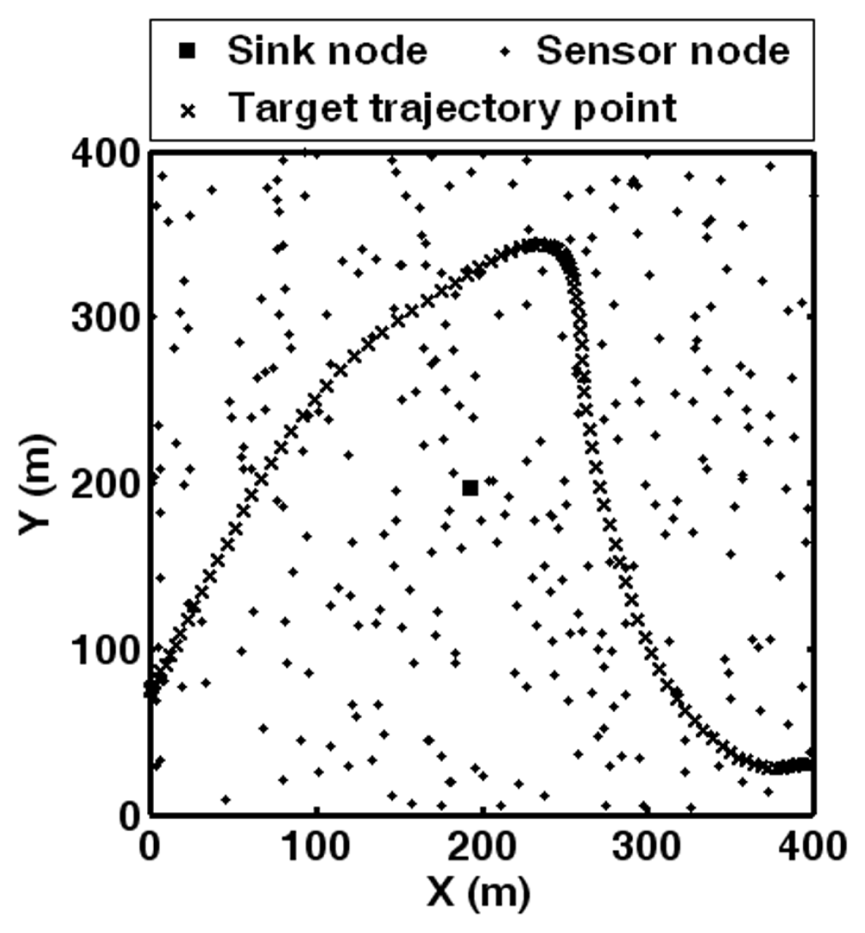
It is assumed that the sensing field of WSN is 400 m × 400 m, in which 300 sensor nodes are deployed randomly. The sensing period is 0.5 s. For the target, maximum acceleration is 5 m/s2 and maximum velocity is 25 m/s. Deployment of WSN and target trajectory is given in Figure 2. The trajectory of 100 points involves different moving situations, so this scenario can represent the generalization of tracking problem. According to Section II, each sensor node has the sensing range of 40 m. The standard deviation of bearing observations is 2° while that of range observations is 1 m. The parameters in (5) are set as: α1 = 500 nJ/bit, α2 = 5 nJ/(bit · m2) and rd=1 Mbit/s. The data amount of observations is 1 KB for each sensor node. It is assumed that the time for staying in each mode is δt = 20 ms .Then, the power consumption of WSN in the each sensing period is:
where T is the sensing period and k is the sensing period index. P(i,k) denotes the power consumption of sensor node i in the k -th sensing period. Moreover, the total energy consumption of WSN after nT sensing periods is:
Among the total energy consumption, energy consumed by transmission portion is defined as transmission cost, while the other energy consumption is defined as the operation cost.
5.2 Target Tracking Experiments
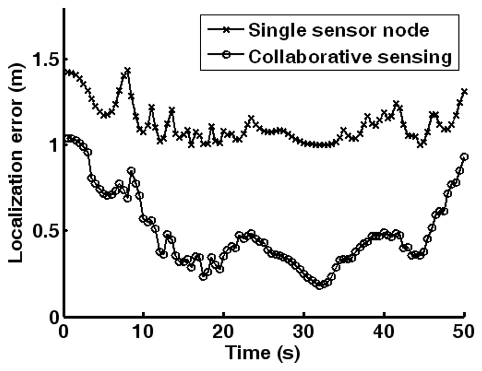
First, the efficiency of collaborative sensing is discussed. For sensing performance comparison, we consider the situation that only the closest sensor node for the target acquires the observations. Figure 3 compares the target location error with collaborative sensing and single sensor node. Obviously, the localization errors of single sensor node and collaborative sensing method have the same trend, where are impacted by the same obstacles and noises. However, it can be seen that the collaborative target location error is much less than that of single sensor node all the time. The reason is that the collaboration of multiple sensor nodes can enhance the tracking ability and weaken the impact of noise and obstacles, which can significantly improve the robustness of target tracking. Thus, the sensing performance is enhanced by the collaborative sensing.
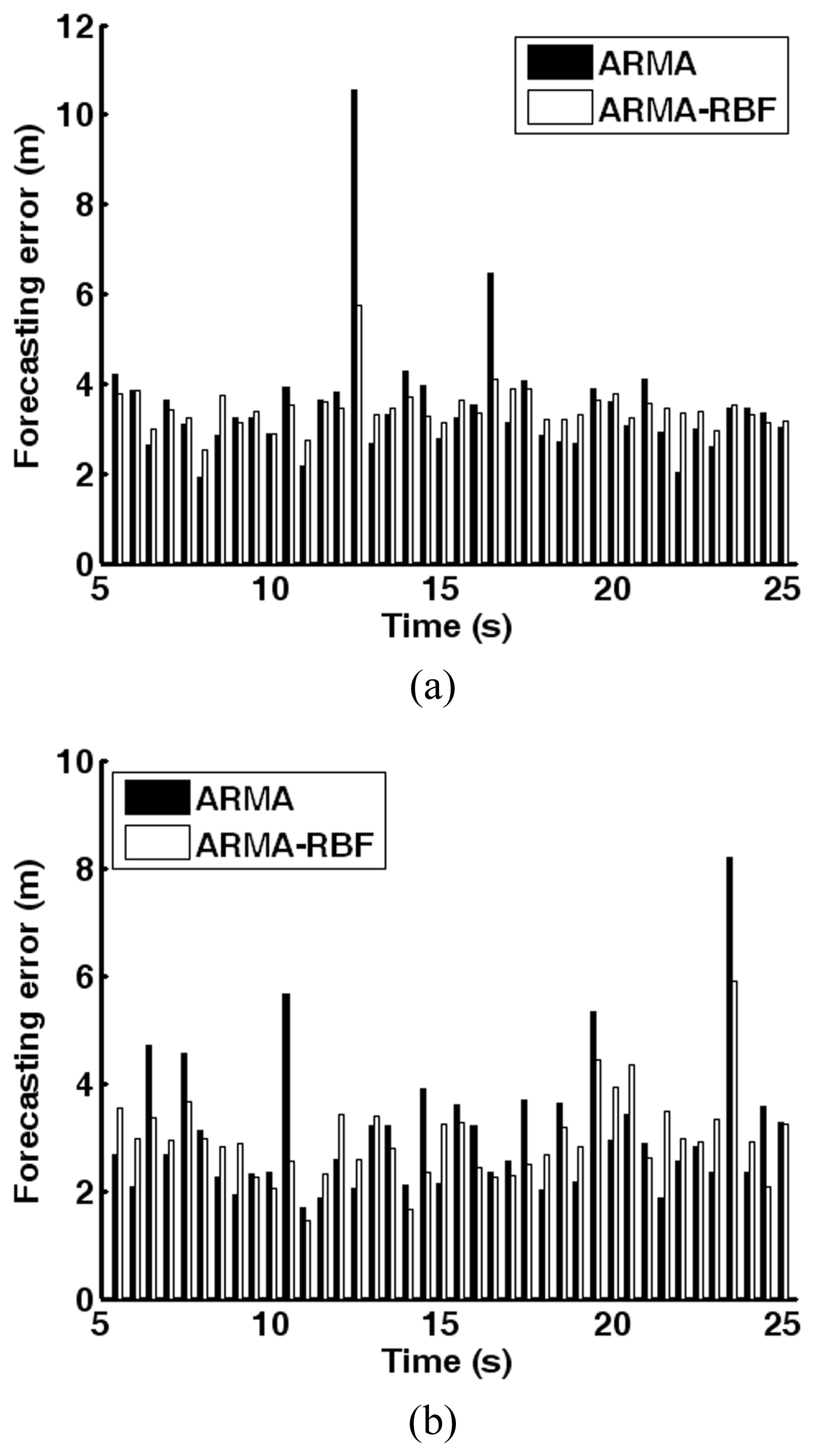
Then, the target position forecast performance of time series analysis is studied. In each sensing period, the known target trajectory in the x and y directions forms two sets of time series, which are analyzed respectively without further assumptions. It is assumed that target localization in the initial 5 s can be guaranteed by the boundary sensor node, where the target localization results are used for ARMA learning. According to Section III, the target positions forecasting error with ARMA and ARMA-RBF is compared. The forecasting error from 5 s to 25 s is given in Figure 4. Following the patterns of ACF and PACF, the parameter p is set as 3 for AR(p) model. As illustrated in Figure 4, because RBFN is dynamically trained and used for compensating the forecasting error of ARMA model, the forecasting error of ARMA-RBF algorithm is much less than ARMA algorithm. Thus, with ARMA-RBF algorithm, the estimation of target movement can provides more accurate results for sensor nodes scheduling. Obviously, the energy-efficient organization method can stably keep the energy consumption of operation and transmission in a low level. It means that the energy consumption of WSN can be more balanced, and the lifetime of whole WSN can be prolonged, with the guidance of energy-efficient organization.
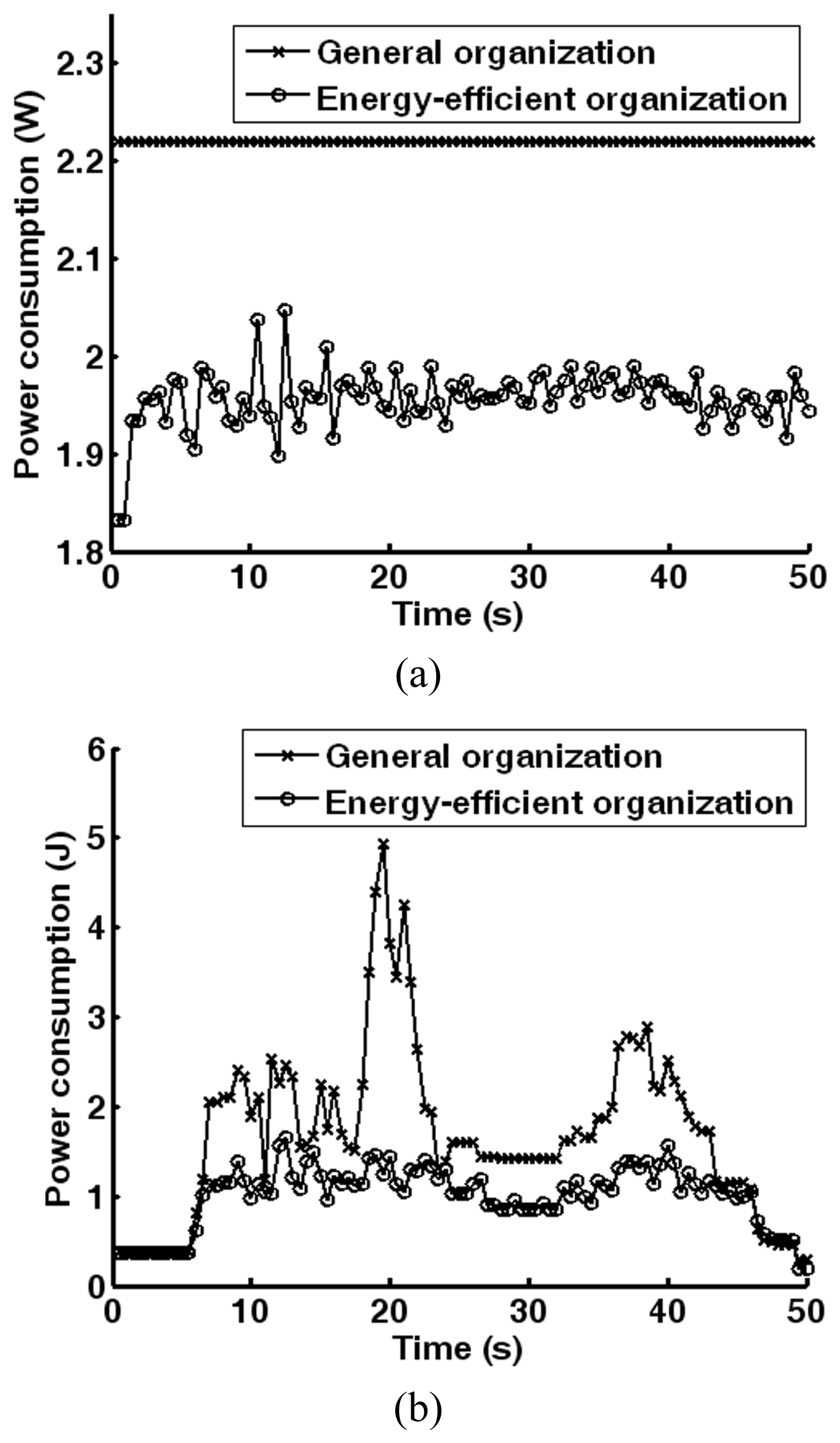
With the forecasted target position, the sensor nodes estimate the sleep period number and go to sleep in a distributed manner. Thereby, the operation cost of WSN is optimized. In each sensing period, all the sensor nodes which can detect the target wake up. In order to minimize the transmission cost, the ACO algorithm is utilized for routing. According to (25), the power consumption of WSN is calculated. Meanwhile, a general organization approach is considered for comparison, where all the sensor nodes wake up every sensing period. Instead of ACO algorithm, sensor nodes forward their observations according to the distance from sink node, where it starts on farthest sensor node and ends on the closest sensor node. Figure 5(a) illustrates the operation cost with general organization and energy-efficient organization, while the power consumption curves of transmission cost are presented in Figure 5(b). Utilizing energy-efficient organization, the operation and transmission costs are both lower, because the energy-efficient organization method can automatically adjust the status of sensor nodes and schedule the sleep period of each sensor node according to the estimation of target movement.
According to Figure 5, Table 1 gives the energy consumption of the organization approaches utilizing (26). Define the relative reduction of energy consumption as:
where
and
denote the energy consumption with general and energy-efficient organization, respectively. Thus, 12.3% operation cost and 40.7% transmission cost is saved during target tracking.
6. Conclusions
Considering the energy constraints of target tracking in WSN, this paper proposes an energy-efficient organization method based on collaborative sensing and adaptive target estimation. Sensor nodes which are equipped with bearing and range sensors utilize the maximum likelihood estimation for data fusion. Hence, targets can be localized by collaborative sensing while the localization error is evaluated utilizing FIM. A sink node maintains the historical target positions, with which the target position in the next sensing instant is estimated by ARMA-RBF. The future target position is derived from the forecasted results and is adopted to organize the sensor nodes for sensing. Here, the energy-efficient organization method includes the distributed sensor node awakening and adaptive routing scheme. Sensor nodes can go to sleep when there is no target in its sensing range and it can be awakened once there is potential sensing task. Besides, probabilistic awakening is introduced to prolong the sleep time of sensor nodes. ACO algorithm is employed to optimize the path of data transmission. Experiments of target tracking verify that target localization accuracy is enhanced by collaborative sensing of the sensor nodes, while the forecasting performance is improved by combining ARMA model and RBFN. More importantly, the energy efficiency of WSN is guaranteed by the distributed sensor awakening and dynamic routing. The main contribution of this paper is an energy-efficient organization framework for target tracking as well as the forecasting and awakening approaches.
Acknowledgments
This paper is supported by the National Basic Research Program of China (973 Program) under Grant No. 2006CB303000 and National Natural Science Foundation of China under Grant #60673176, #60373014 and #50175056.
References and Notes
- Sinha, A. Dynamic power management in wireless sensor networks. IEEE Design and Test of Computers 2001, 18, 62–74. [Google Scholar]
- Duh, F.B.; Lin, C.T. Tracking a maneuvering target using neural fuzzy network. IEEE Transactions on System, Man, and Cybernetics 2004, 34, 16–33. [Google Scholar]
- Wang, X.; Wang, S.; Ma, J. An improved particle filter for target tracking in sensor system. Sensors 2007, 7, 144–156. [Google Scholar]
- Oshman, Y.; Davidson, P. Optimization of observer trajectories for bearings-only target localization. IEEE Transactions on Aerospace and Electronic Systems 1999, 35, 892–902. [Google Scholar]
- Zhang, H. Optimal and self-tuning State estimation for singular stochastic systems: a polynomial equation approach. IEEE Transactions on Circuits and Systems 2004, 51, 327–333. [Google Scholar]
- Lee, M.J.; Choi, Y.K. An adaptive neurocontroller using RBFN for robot manipulators. IEEE Transactions on Industrial Electronics 2004, 51, 711–717. [Google Scholar]
- Zecchin, A.C. Parametric study for an ant algorithm applied to water distribution system optimization. IEEE Transactions on Evolutionary Computation 2005, 9, 175–191. [Google Scholar]
- Wang, X.; Wang, S. Collaborative signal processing for target tracking in distributed wireless sensor networks. Journal of Parallel and Distributed Computing 2007, 67, 501–515. [Google Scholar]
- Wang, X.; Ma, J.; Wang, S.; Bi, D. Prediction-based dynamic energy management in wireless sensor networks. Sensors 2007, 7, 251–266. [Google Scholar]
- Biscainho, L.W.P. AR model estimation from quantized signals. IEEE Signal Processing Letters 2004, 11, 183–185. [Google Scholar]
- Haykin, S. Neural Networks: a Comprehensive Foundation; Prentice Hall: NJ, USA, 1999. [Google Scholar]
Figure 1.
The framework for ARMA-RBF forecasting.

Figure 2.
Deployment of WSN and the target trajectory.

Figure 3.
Comparison of target localization error with collaborative sensing and single sensor node.
Figure 3.
Comparison of target localization error with collaborative sensing and single sensor node.

Figure 4.
Target position forecasting error of ARMA and ARMA-RBF in the coordinate frame XOY: (a) X direction; (b) Y direction.
Figure 4.
Target position forecasting error of ARMA and ARMA-RBF in the coordinate frame XOY: (a) X direction; (b) Y direction.

Figure 5.
Power consumption comparison with general organization and energy-efficient organization: (a) operation cost; (b) Transmission cost.
Figure 5.
Power consumption comparison with general organization and energy-efficient organization: (a) operation cost; (b) Transmission cost.


| Energy consumption (J) | General organization | Energy-efficient organization |
|---|---|---|
| Operation | 111.5 | 97.8 |
| Transmission | 84.7 | 50.2 |
© 2008 by MDPI (http://www.mdpi.org). Reproduction is permitted for noncommercial purposes.
Share and Cite
MDPI and ACS Style
Wang, X.; Wang, S.; Ma, J.-J.; Bi, D.-W. Energy-efficient Organization of Wireless Sensor Networks with Adaptive Forecasting. Sensors 2008, 8, 2604-2616. https://doi.org/10.3390/s8042604
AMA Style
Wang X, Wang S, Ma J-J, Bi D-W. Energy-efficient Organization of Wireless Sensor Networks with Adaptive Forecasting. Sensors. 2008; 8(4):2604-2616. https://doi.org/10.3390/s8042604
Chicago/Turabian StyleWang, Xue, Sheng Wang, Jun-Jie Ma, and Dao-Wei Bi. 2008. "Energy-efficient Organization of Wireless Sensor Networks with Adaptive Forecasting" Sensors 8, no. 4: 2604-2616. https://doi.org/10.3390/s8042604